
A Review of Dynamic Models of Hot-Melt Extrusion


Service d’Automatique, Université de Mons, 31 Boulevard Dolez, 7000 Mons, Belgium
*
Author to whom correspondence should be addressed.
†
These authors contributed equally to this work.
Processes 2016, 4(2), 19; https://doi.org/10.3390/pr4020019
Submission received: 31 January 2016
/
Revised: 7 May 2016
/
Accepted: 21 May 2016
/
Published: 6 June 2016
Abstract
:Hot-melt extrusion is commonly applied for forming products, ranging from metals to plastics, rubber and clay composites. It is also increasingly used for the production of pharmaceuticals, such as granules, pellets and tablets. In this context, mathematical modeling plays an important role to determine the best process operating conditions, but also to possibly develop software sensors or controllers. The early models were essentially black-box and relied on the measurement of the residence time distribution. Current models involve mass, energy and momentum balances and consists of (partial) differential equations. This paper presents a literature review of a range of existing models. A common case study is considered to illustrate the predictive capability of the main candidate models, programmed in a simulation environment (e.g., MATLAB). Finally, a comprehensive distributed parameter model capturing the main phenomena is proposed.
1. Introduction
Hot-melt extrusion has been a forming technique in popular use in industry since the 19th century. It is a thermomechanical manufacturing process where solid materials are transformed into a uniform product with a specific, possibly complex, shape by forcing passage through a die [1]. Besides the die, the process includes a conveying system, involving the rotation of a screw (or several screws), such that the material is transported by an Archimedean screw action through the device. Nowadays, more and more forming processes use this technique, and the products that can be extruded are numerous: plastics [2,3], drugs [4,5,6,7], food [8,9,10], metals [11,12], tissue engineering scaffolds using electrospinning [13,14,15], porous items using supercritical fluid [16], etc.
A discontinuous extrusion process, which is also widely used in industry, is the ram extruder, where the whole material billet is directly injected into the device and pushed out from the die by the ram pressure [17]. This single or multi-ram batch process can generate extremely high pressures, but usually results in poor melting efficiency [18]. In the following, this type of process will not be discussed, and attention will be focused only on modeling twin screw systems.
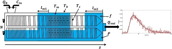
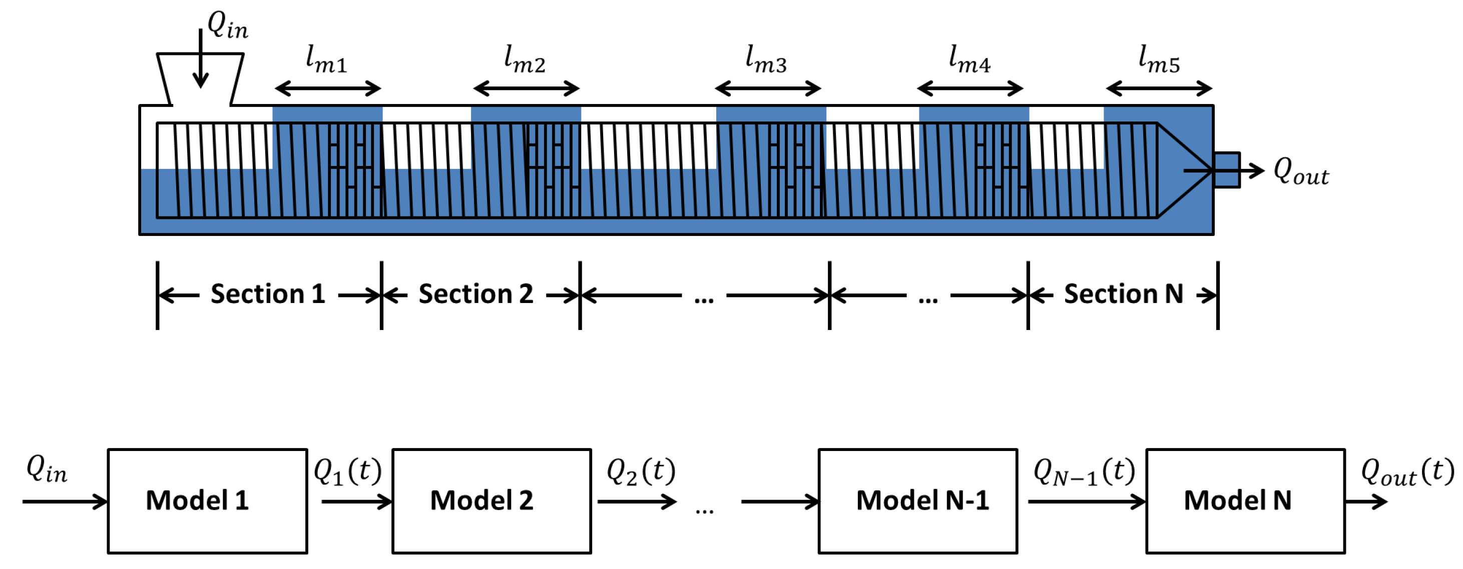
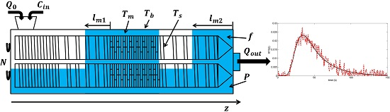
Hot-melt extrusion is a complex process, as it involves an assembly of different screw elements (forward element, reverse element, kneading block) to manufacture the end product. The selection of the design parameters of the screw and the operating conditions of the process, including the screw rotation speed N, the barrel temperature , the feed flow rate of material and the component concentration (see Figure 1), offer a wide range of possibilities. In turn, this multivariable process is characterized by a set of internal state and output variables, including material filling ratio f, pressure P, material temperature , screw temperature , die flow , etc. (see Figure 1). To regulate the process around the desired operating point, a control system is usually required [19,20,21,22,23,24].
The aim of this paper is to review the mathematical models of hot-melt extrusion that were proposed in the past few decades, with a focus on dynamic models that could be the basis for developing a simulator, a state estimator or a controller. The reviewed models range from simple continuous-stirred tank reactors (CSTRs) in series to sophisticated distributed parameter models, involving mass and energy partial differential equations (PDEs). The interesting approaches of population balance modeling (PBM) and discrete element modeling (DEM) are addressed, and purely data-driven, black-box models, are also considered.
In order to not restrict the review to a purely theoretical descriptive point of view, a simple case-study is considered to benchmark the main model candidates. To this end, dynamic simulators are developed in the MATLAB environment. As a result, a dynamic PDE model is proposed as a relevant model of the extrusion process.
This paper is organized as follows. The next section introduces the case study that will be used to illustrate and test the main modeling approaches. Section 3 presents several explicit models describing the residence time distribution (RTD) in the extrusion device, while Section 4 discusses dynamic models based on a discretization of the system in CSTRs and differential equation (ODE) models. Partial differential equation (PDE) models are then reviewed in Section 5. Section 6 provides a brief introduction to PBM and DEM, while a review of black-box models, i.e., transfer function models and neural network models, is presented in Section 7. The last section of this paper draws the main conclusions.
2. A Simple Case Study
A simple case study is used as a benchmark in this article, so as to illustrate the main modeling paradigms. It consists of a twin screw with the same pitch all along the device (see Figure 2). The geometrical and physical parameters are listed in Table 1. Moreover, this table gives the parameters of the empirical equations selected to model the material rheological behavior. Various studies were dedicated to the evolution of material characteristics, such as the viscosity, melt density, size and shape distribution of the particle clusters, electrical properties and evidenced complex dependencies with respect to the degree of mixing, the quantity of air into the extruded compound, etc. [25,26,27,28,29,30,31,32,33]. For some extruded materials, analytical studies do not allow one to obtain an accurate representation of the rheological properties, and in-line measurements from an actual extrusion device are required [34]. Rheological properties largely contribute to the nonlinear process behavior. In our case study, only the shear viscosity variations are considered, and Yasuda–Carreau equations, which are functions of the shear rate and the temperature with four adjustable parameters, are employed (see, for instance, [35,36,37]). They are described by the following equations:
where is the zero shear viscosity, the characteristic matrix time constant, the shear rate, a the Yasuda parameter and the pseudo-plastic index. The dynamic zero shear viscosity is varying with the material temperature T following the Arrhenius law:
Using one of the most elaborate models [38], which is presented in detail in Section 5, a simulation code is implemented in MATLAB. The partial differential equation model is discretized using four-point finite differences with 150 nodes, and time integration is performed with the solver . A residence time distribution (RTD) test is simulated with a screw speed rotation RPM (revolution per minute) and a feed flow rate kg/h. An additive Gaussian white noise with a standard deviation of is considered, to represent the situation where the RTD is measured using tracer and colorimetric techniques [39]. The resulting RTD is represented in Figure 3.
3. The Earlier Models: Static Maps
Basically, extrusion enhances component mixing. A fundamental process characteristic is the time spent in the extruder by the several components of interest, which can be assessed thanks to an RTD, as shown in Figure 3. According to [9,40], the RTD signal reflects the process operating conditions, such as the material homogeneity, the uniformity degree of particle shearing, the calorific exchanges (input barrel temperature or outside thermal flux changes) depending on the screw rotation speed, the feed flow rate, etc. The capacity of a model to predict the RTD of each component is therefore important to check that mixing, and possibly the chemical reaction, is achieved before the die. The analysis of the RTD shape leads to a general description of the flows inside the device. Consequently, monitoring this output is particularly important during process scale-up [41].
Earlier modeling works focused on an explicit representation of the RTD (see [42,43]). The first extrusion models, as reviewed in [44], consider and combine two types of reactors with a priori known RTDs (see Figure 4):
- Plug flow reactors characterized by a uniform residence time distribution for all particles.
- Continuous stirred-tank reactors (CSTRs) assuming the non-uniformity of the residence time, but a uniform composition of the flow.
Based on these building blocks, the first model consists of a cascade of CSTRs (see Figure 5), while the second model structure combines a plug flow reactor with a cascade of CSTRs.
The mathematical model corresponding to these structures can be expressed in the form of Equation (3):
where is the plug flow effect and is the ratio between the diffusive and the convective effects. is the minimum residence time; is the mean residence time; n is the number of reactors; and is a dimensionless time variable.
Parameter identification based on RTD experimental data is straightforward, but the model fit is not always satisfactory [45], particularly with the plain CTRs-in-series model. The plug flow model compartment is often required and can improve the data reproduction to some extent [45,46].
The selected number n of reactors varies significantly with the application, from eight in chocolate manufacturing [46] to 500–900 for a granulation process [45]. The reader is referred to the works [47,48] where the appropriate number of reactors is determined for different screw elements based on a thermo-mechanical partial differential equation (PDE) modeling.
These preliminary observations demonstrate that the physical phenomena occurring in an extrusion process are difficult to model. For instance, the die shape causes obstructions, resulting in leakage flows and material stagnancy. Efforts were therefore deployed in order to consider these aspects (mathematical expressions are not included in the text for the sake of conciseness):
- The work in [49] models the RTD of wheat flour particles using five volume elements of different sizes, each sub-divided in a series of CSTRs with identical volumes. In order to represent the tail in the RTD, three reactors with backward flows are included so as to explain material accumulation at the die (see Figure 6).
- The work in [50] uses a combination of a plug flow reactor with a cascade of CSTRs with the same volume and a backward flow (see Figure 7). The plug flow reactor represents the feeding zone and is characterized by a delay . The cascade of CSTRs models the completely filled part inducing a reflux and characterized by two parameters: the number of reactors n and the ratio between the forward and backward flows .
The earlier models (which at least find their roots in earlier works, some of them having been proposed relatively recently) are therefore static maps based on RTD calculation reflecting the operating conditions (screw configuration, screw rotation speed, feed flow rate, etc.) linked to the desired end-product quality.
To illustrate their potential, the model of [51] is used to represent the RTD measurements of Figure 3. Equation (3) is modified to include a dead zone parameter d, which influences parameter .
A least-squares cost function is defined in order to estimate the unknown parameters through the solution of the following problem:
The estimated parameters are listed in Table 2, and a model direct validation is presented in Figure 9, which is quite satisfactory.
Static maps are limited in scope and do not offer much potential in terms of process control. The next section therefore pays attention to differential equation models, based on similar decomposition of the extrusion device into specific elements, such as CSTRs.
4. Reactors-In-Series Approach
The reactors-in-series approach is a direct extension of the previous concepts, i.e., it is based on a decomposition of the extrusion device into volume elements where perfect mixing is assumed, but dynamics are now taken into account. Based on mass and energy balances and on rheological laws, variations of the main state variables, such as filling ratio (ratio between the volume occupied by the material over the available mixing volume; a value of one represents a completely filled screw channel section and less than one a partially filled screw channel section), pressure, temperature and monomer concentration, can be represented by ordinary differential equation systems (ODEs).
Mass balances essentially allow one to determine the filling ratio of each reactor based on the inlet () and outlet () mass flows. Considering n reactors, mass balances are written as follows:
where i is the reactor index, ρ is the material density and and are the respective volume and filling ratios.
Mass balances can also be used to determine the reacting monomer concentration, as in:
where M is the molar mass of the monomer, the inlet monomer concentration, the concentration of monomer in reactor i and R the reaction rate.
Temperatures can be determined on the basis of energy balances involving several heat transfer mechanisms: convective heat transfer, heat exchange between the screw elements and chemical reaction heat. In many works [35,52,53,54,55], viscous friction dissipation is also included in the energy balance. The computation of the barrel and screw temperatures is possible, but for the sake of clarity, only the expression of the material temperature is given here:
where is the mass of material in reactor i, the specific heat capacity, and the heat exchange coefficients between material/barrel and material/screws, respectively, and the exchange surfaces between material/barrel and material/screws, respectively, r the reaction rate and the reaction enthalpy.
Since density and shear viscosity enter into the expressions of the flow and viscous friction dissipation, rheological properties of the material should be included in the process model. In the literature, a constant density is often used and the shear viscosity is modeled by an empirical equation [56,57,58] or a rheological law [35,52,53,54,55].
The reactors-in-series models can be classified into two categories depending on whether specific sections of the screws (C-chamber, inter-meshing element, kneading block) are represented by a CSTR. A classifying review of the existing models is achieved in the following.
- Models with Predetermined Screw DiscretizationIn [56,57], the filling ratio, monomer concentration, temperatures and RTD are determined for a counter-rotating twin screw extruder using a subdivision of the screws in C-chambers (see Figure 10) where mass and energy balances are expressed using continuum mechanics. If the system includes a high inter-meshing area between the screws, other volume elements may be added to model the specific flows in this zone (see [52]).An extrusion device presents a varying filling level, a function of the local screw geometry. It is generally considered that an extruder comprises two different zones, which can be partially or completely filled, inducing specific mass balance expressions. Indeed, mass flow networks are different in each zone. In partially-filled zones, only a pumping flow , due to the screw rotation, transports the material along the section. In completely filled zones, the presence of a pressure gradient creates leakage flows, and the resulting mass flow network is modeled by parallel C-chambers, in which the leakage locations are divided into five groups [59] (see Figure 11):
- −
- the flight gap (with flow ) between the barrel and the screw flight;
- −
- the tetrahedron gap () between the flight walls;
- −
- the calender gap () between the flight of one screw and the bottom of the other screw channel;
- −
- the side gap () between the flanks of the two screws flight;
- −
- the channel gap () down-channel flow in the screw channel.
- Models with Adjustable DiscretizationIn [35,53], the different screw sections can be discretized using an adjustable number of CSTRs (see Figure 12). Material can flow in the forward direction, with flow due to the screw rotation, and in the backward direction, with flow due to the pressure difference between two reactors, as shown in Figure 12 and Table 3 [60].Based on the filling ratio, the pressure in each reactor can be computed using a simple algebraic method. Two different situations may happen: in partially-filled reactors (), the pressure P matches the atmospheric pressure , and in the completely filled reactors (), the pressure is above the atmospheric pressure; and flow continuity is verified. The problem can therefore be expressed as a system of linear algebraic equations , where is the pressure vector and A a tridiagonal matrix.
As an application example, the model proposed in [35] is selected to represent the data provided in Figure 3. Three parameters have to be estimated: the number of reactors n and two flow geometric correction factors , , for the forward and backward flow (these latter parameters are multiplicative factors of the screw geometric parameters and and take into account the assumption that screw channels are rectangular in shape).
The estimated parameter values are given in Table 4, and direct validation is illustrated in Figure 13, which is obviously a better fit to the experimental data than Figure 9.
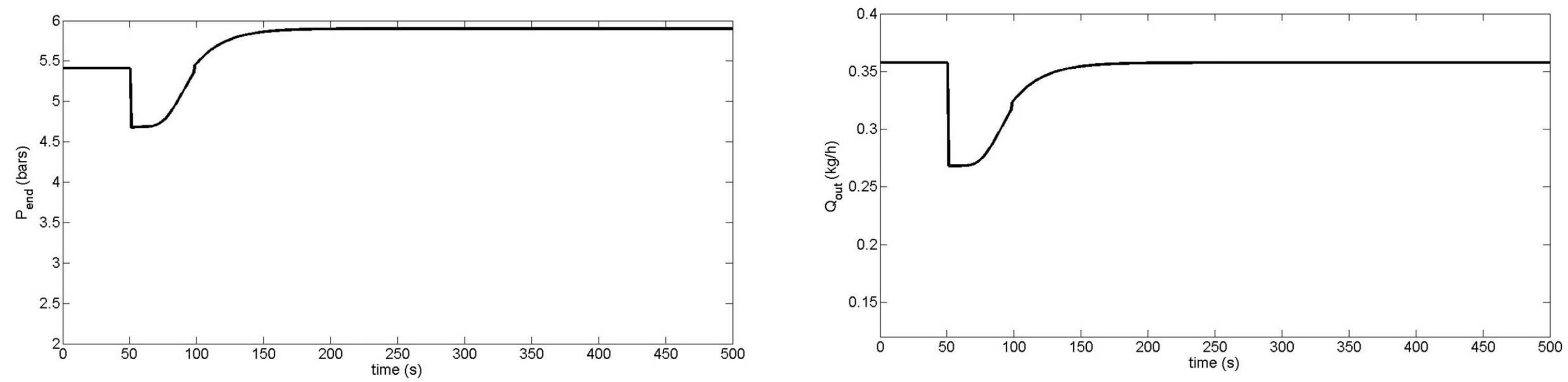
An additional advantage of ODE models is the possibility to simulate various scenarios. For example, the effect of step changes in the inputs can be easily studied, e.g., a step change in the screw speed rotation N from 100 down to 75 RPM and a step-change in the feed flow from down to kg/h. The choice of as an input includes the use of the “starve-fed” mode where the flow is precisely controlled by loss-in-weight feeders. It should be noted that “flood feeding”, where the screw rotation speed controls the flow rate, can be another method to produce feeding profiles. The process outputs, e.g., the die pressure and the outlet flow , are presented in Figure 14 and Figure 15, respectively.
These results show that dynamical analysis of the extrusion system can be easily performed. However, model accuracy is still perfectible in several aspects. For instance, poor agreements between simulation and experimental data at a low screw rotation speed have been reported in [56] or a discrepancy of the influence of the screw rotation speed on the pressure die has been observed in [52]. This motivates the exploration of distributed parameter models, involving mass and energy balance partial differential equations.
5. Distributed Parameter Models
The direct formulation of mass, energy and, possibly, momentum balance partial differential equations (PDEs) is an appealing alternative to the use of the CSTR-in-series paradigm, where there is an interplay between the model definition and the numerical solution via the number of reactors. Distributed parameter models allow the uncoupling between model formulation and solution techniques, which can be of arbitrary sophistication (finite differences, spectral methods, finite volume methods, etc). Depending on the modeling assumptions, i.e., 1, 2 or 3 spatial dimensions, a (non-)Newtonian fluid, (non-)isothermal conditions, many different model formulations are possible.
3D models are presented, for instance, in [61,62,63,64,65,66,67,68,69,70,71,72,73,74,75,76,77,78,79,80,81,82]. These models are solved using classical computational fluid dynamics (CFD) tools, such as finite element or finite volume methods.
These models can include all of the features already discussed in this article, such as a description of the changes in the rheological properties of the material along the device, the presence of partially- or completely-filled zones, the wall slip effect on the flows [83,84,85,86,87], etc. The resulting 3D models can be used to achieve some dynamic studies, such as the analysis of the instabilities of the die flow [88,89] or the description of the chaotic motion inside screw elements by dynamic tools (Lyapunov exponents, Poincare sections and particle tracking), which enable the study of the mixing conditions in hot-melt extrusion processes [90,91,92]. However, the numerical solution of the conservation laws requires important computational effort, and 3D CFD will be mostly useful for system design and steady-state analysis.
The work in [93] presents a comparison between a 3D and 1D PDE model of a specific extrusion device. For dynamical study and model-based control, 1D representations will usually be more appropriate. Among the works considering a 1D axial representation, one can note [94,95,96,97,98,99,100,101,102]. In these works, the spatial profiles of the filling ratio, pressure and temperature along the different screw elements are studied in steady state. However, most of them could be applied for transient computation, as well.
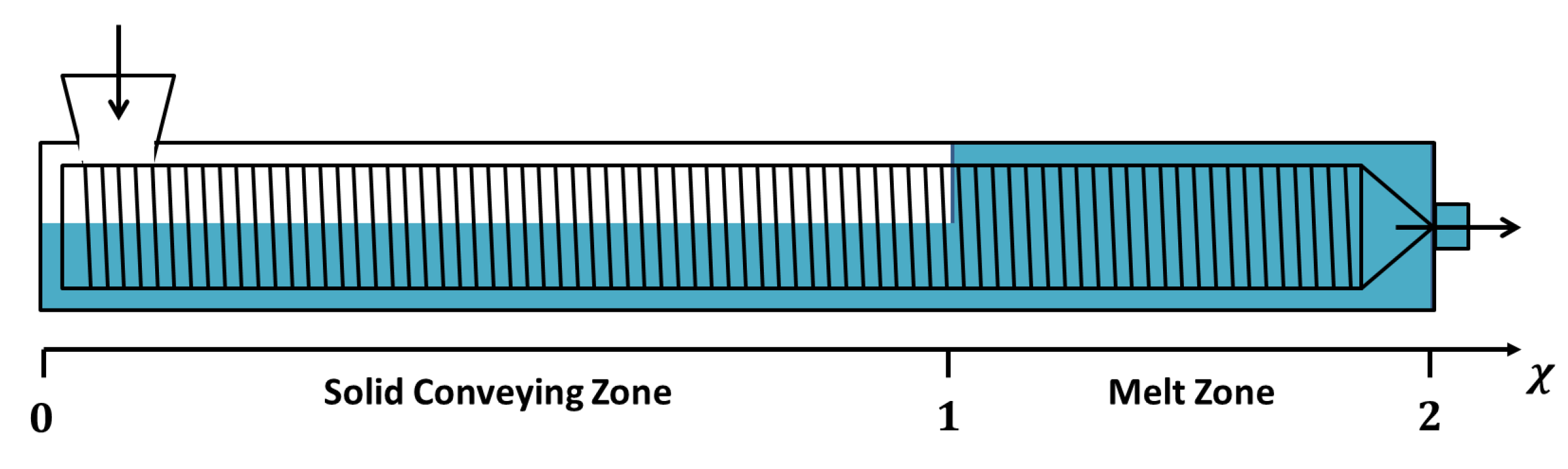
The literature shows that many 1D dynamical models are based on [38], in which the system is divided into two specific zones: the solid conveying zone (SCZ) and the melt zone (MZ) (see Figure 16). Steady state analyses of such models are achieved in [103].
Specific balance equations are used in the different zones:
- Solid conveying zone:This zone is characterized by a varying filling ratio . Material accumulates or flows along this zone during the transient period. Mass and energy balances are therefore expressed by the following equations:
- −
- Mass balance:where ξ and N are respectively the screw pitch and rotation speed.
- −
- Energy balance:where T is the material temperature, ϕ the viscous energy dissipation factor, a geometric parameter characterizing the viscous energy dissipation [104], the viscosity, ρ the density, V the shear volume, the specific heat capacity, the convective heat transfer coefficient, the equivalent circumference of the twin screw and the barrel temperature.
- Melt zone:Unlike the solid conveying zone, the forward flow is considered as constant since the density itself is constant and the zone completely filled. In the following equations, the backward flow is associated with the pressure flow between two parallel plates assuming that the screw gaps are much smaller than the screw diameter. The net flow rate at any location in the melt zone equals the output flow at the die, . The mass and energy balance equations are:
- −
- Mass balance:where B is a constant governing the leakage back flow and P the pressure.Determination of this pressure is possible using the following equation:
- −
- Energy balance:where is a geometric parameter characterizing the viscous energy dissipation [104] and η is the viscosity. U is the convective heat transfer coefficient.
Due to the existence of two zones, a boundary condition at the moving interface must be expressed. During the transient period, the melt zone length () changes. This can be explained by an overall mass balance of the melt zone:
where is the melt zone length, is the filling ratio at the melt zone inlet, is the inlet mass flow rate in the melt zone and is the output die flow rate. represents volume free from material. An ODE is formulated to determine the melt zone length:
This dynamic model results in a PDE system coupled to an ODE describing the moving boundary between the solid conveying zone and the melt zone. The movement of this separation involves the zone description (solid conveying or melt), its discretization and the associated balance change during time. The application of standard numerical techniques is therefore difficult, and an alternative method is preferred. The principle of a simplified solution procedure is represented in Figure 17.
The suitability of this model [38] has however not been tested in a more realistic screw configuration (e.g., more complex geometry, presence of kneading blocks, etc). In real applications, the screw geometry discontinuity involves a discontinuous filling ratio f evolution, which can cause numerical problems. The authors of [105] alleviate this by focusing on a continuous variable: the net flow rate Q. In a configuration with reverse pitch sections, they propose a mass balance equation allowing the determination of Q:
To tackle the problem of a moving interface between the partially- and completely-filled zones, [106] suggests the introduction of a new spatial variable χ ranging from 0–2 (see Figure 18). The solid conveying zone is delimited by the interval [0,1], and the spatial variable is expressed as . In the melt zone, the new variable is restricted to the interval [1,2] by . These changes of variable are convenient as they transform a PDE problem with a moving boundary into a PDE problem on fixed spatial domains, which makes spatial discretization easier to implement.
In this review, a dynamic model is implemented based on these recent works and, notably, the work in [38]. The filling ratio, pressure and temperature are modeled using a division of the device in two zones, and an ODE is added to the equation system to determine the moving interface. Using the method of lines (MOL) [107] with a four-point finite difference scheme on a spatial grid with 150 nodes and the ordinary differential equation solver , numerical solutions can be computed accurately. To reproduce a tracer concentration, such as the one used in the RTD test, Equation (16) is used:
where C is the tracer concentration, Q the net flow rate and D the diffusion coefficient.
The data provided in Figure 3 is used to estimate the parameters in Equations 8–14 and 16, e.g., the shear volume V, a constant governing the leakage back flow B and the diffusion coefficient D. These unknown parameters are identified using a least-square cost function similar to 4. Estimated parameter values are summarized in Table 5, and a direct validation is presented in Figure 19. The estimated parameters actually correspond to those used in the original simulator, which generated the RTD “experimental” data. Confidence intervals shown in Table 5 demonstrate that the information content of the RTD signal is sufficient to ensure the practical identifiability of the three considered parameters.
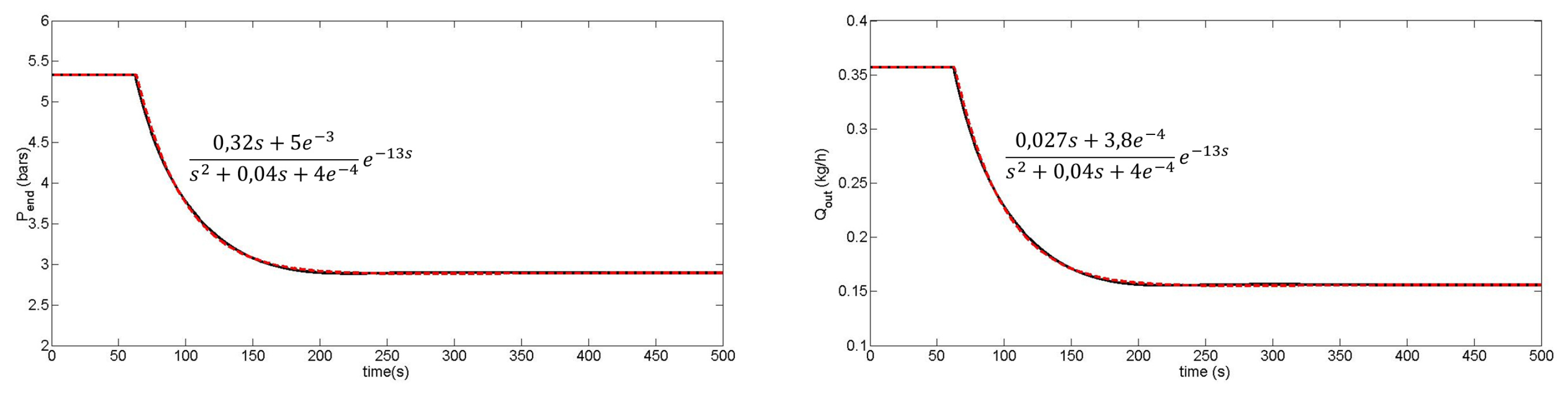
As with the CSTR-in-series model, the time responses to step changes in the input can easily be evaluated, i.e., die pressure and the outlet flow responses to step changes in the screw rotation speed rotation N from 100 down to 75 RPM and in the feed flow rate from down to kg/h. The results are shown in Figure 20 and Figure 21.
6. Population Balance Modeling and Discrete Element Modeling
This article mostly focuses on dynamic modeling of the global characteristics of the twin screw extruder (filling ratio, pressure, temperature). However, some manufacturing processes require specific material properties for their implementation, and the knowledge of their dynamic evolution along the extruder is important. Population balance modeling (PBM) and discrete element modeling (DEM) are two methods dedicated to this kind of problem, which are briefly discussed in this section.
In PBM, the individuals (particles) are characterized by several properties (independent variables), such as size, liquid content, porosity, spatial coordinates, etc, and are involved in several rate processes, such as aggregation, breakage, nucleation and growth. The models consist of integro-differential equations, in one or more dimensions, which can be formulated as [108]:
where represents the number of particles as a function of particle class x and time t. and are respectively the rate of formation or depletion of the particles depending on several rate processes. These rate processes are generally represented by empirical or semiempirical expressions (for instance, [109,110,111,112]), which is one of the main disadvantages of this modeling approach. Experimental data are required to develop and validate these expressions in some restricted operating regions. PBM are used in various areas, such as crystallization [113], powder mixing [114], powder milling [115] and wet granulation [116,117]. In extrusion processes, this method can be employed to compute different material properties, such as the active pharmaceutical ingredient (API) or excipient component concentration [118], the RTD [119], the particle size distribution, the liquid content and the porosity [120,121].
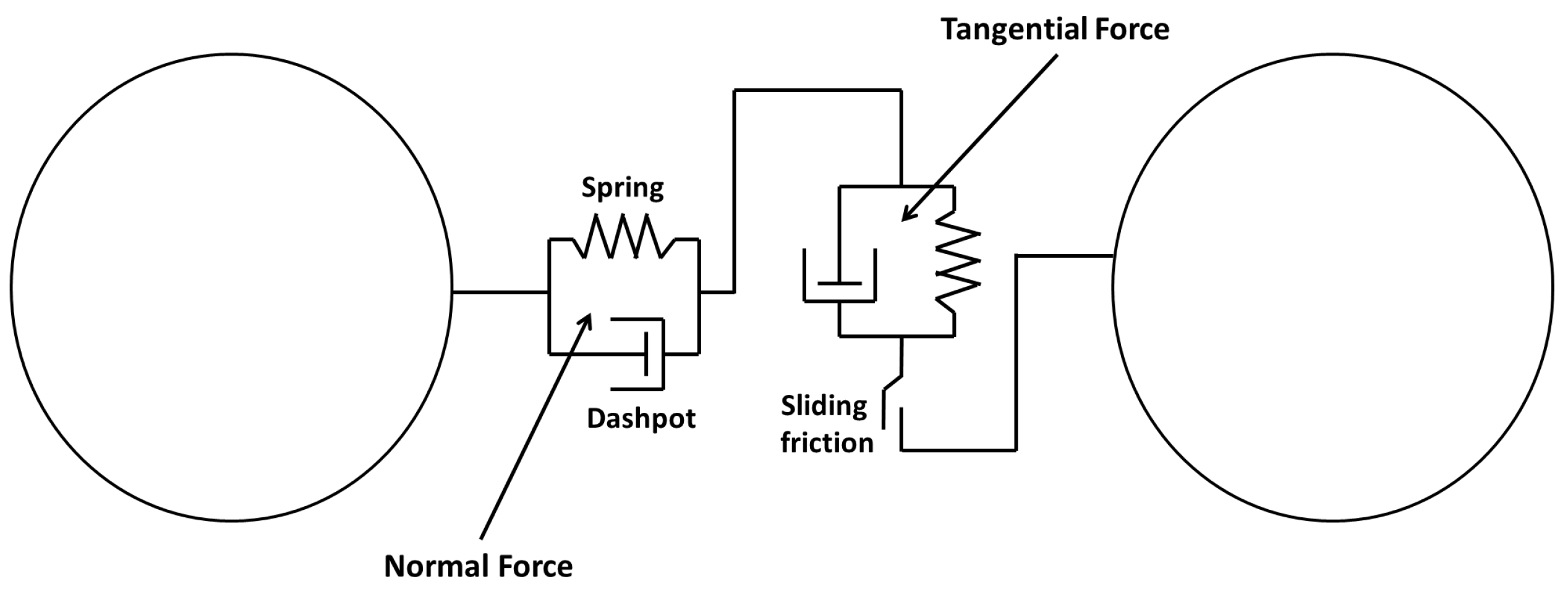
DEM is based on a different approach where each particle is considered as an individual entity [122,123,124,125,126,127]. Two classes can be defined: hard-sphere methods where particles are considered rigid and collisions are instantaneous and binary (note that this method is not valid in twin screw modeling) and soft-sphere methods where interactions upon collisions and lasting contact between the particles and the equipments (screws, barrel) are considered. The implementation of the collisions and contact forces (normal and tangential forces; see Figure 22) in Newton’s second law of motion (Equation (18)) and the angular momentum (Equation (19)) equations at any time instant constitute the modeling.
where v is the particle speed, m the particle mass, g the gravity, I the particle inertia, w the particle angular speed, the force/moment of particle-particle collisions and the force/moment of particle-wall collisions. This method enables the dynamic determination of many variables, such as the collision frequencies, the impact velocities, the pressure, the temperature and the RTD signal, but the computation of each particle requires a high computational effort [128,129,130].
In hot-melt extrusion, influences between some modeled material properties of this section can be observed, and recent works study a coupling PBM-DEM to create an accurate modeling [119,121,131,132,133,134,135]. Figure 23 presents an example (see [136]) of a good combination between these two methods to determine particle physical characteristics. Moreover, computational fluid dynamics (CFD) can also be coupled to PBM-DEM to model particle-fluid interactions in fluidized bed granulation [137,138,139]. However, conversely to the previously-introduced methods, PBM-DEM describes only the variations of particle physical properties (assuming the whole device in the steady state) as the granule size distribution (GSD), the moisture content, etc. [119], and demands huge computational efforts, which are not suitable for parameter estimation and control [124]. Therefore, related simulation studies are not considered in this work.
7. Data-Driven Models
In previous sections, most of the models rely on first principles for their derivation. Depending on their degree of details, they range from “grey-box” to “white-box” models. Conversely, “black box” modeling aims at representing the process by its input-output behavior, with no consideration of the system internal state (see Figure 24).
In the following, two distinct model classes are presented:
- Transfer function models:The input-output behavior of the process around a specific operating point can be described by a transfer function of the form:where and are the Laplace transforms of and , while is defined by a set of parameters () with .There exist many techniques to build transfer function models based on output responses to input solicitations, and some of them are summarized in [140]. Examples of single-screw extruder modeling can also be found in [141,142,143] and serve the development of more specific techniques related to twin-screw configurations, as in [19,20,144,145].Common features of these works include:
- −
- parameter identification based on input step changes;
- −
- first- or second-order transfer functions;
- −
- inclusion of time delays in some input-output relations (feed flow/die pressure, moisture content/die material temperature, etc).
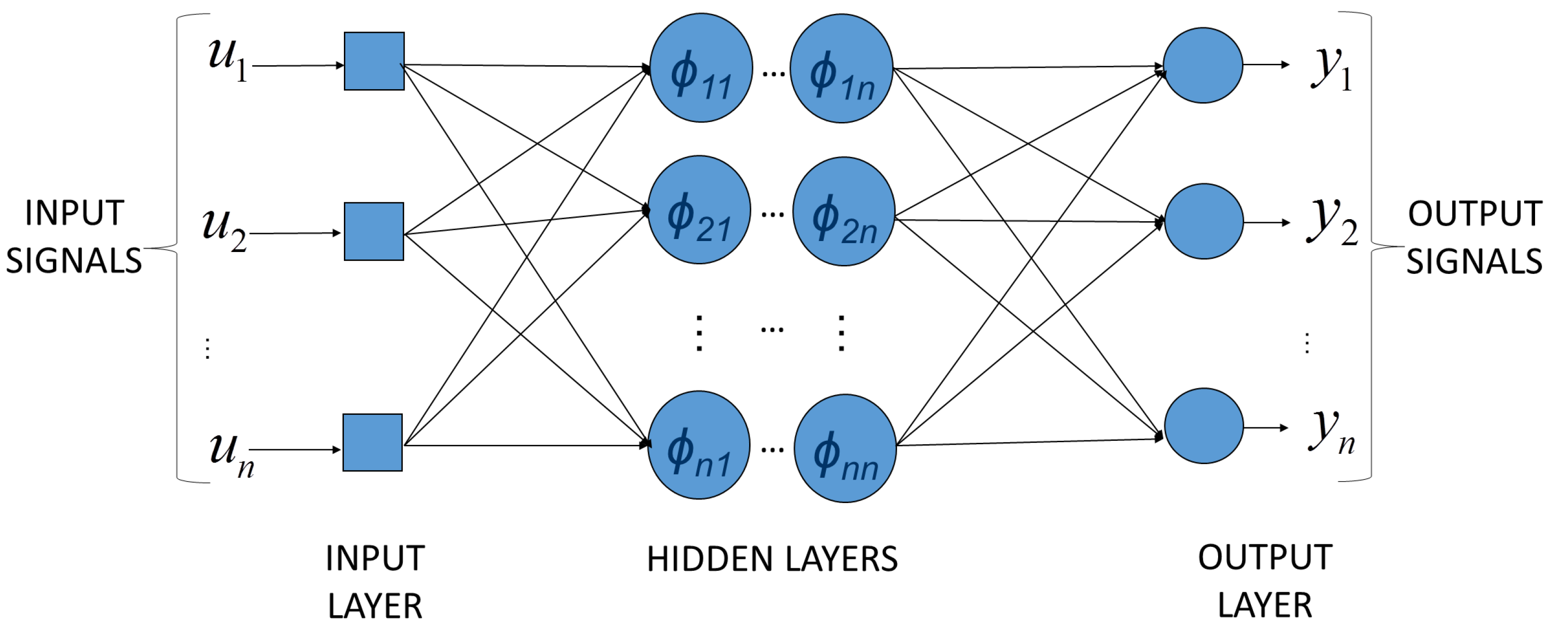
In [146], a comparative study of different parameter identification methods is achieved. Different algorithms are analyzed in the context of cooking extrusion. The couple “screw rotation speed/motor load” supports relay feedback as a well-performing online method, while batch output error parameters provide an accurate modeling across a large range of operating points.The main advantages of transfer function models are their simplicity and the availability of a broad array of well-established control techniques, including PID control. However, transfer function models assume that the process behavior is linear in a limited range of operation. If several distinct operating points have to be considered, different transfer functions will usually have to be identified for each of them. In this latter case, gain-scheduling or adaptive controllers will be required. - Neural networks (NN):Standard feedforward NNs basically define a nonlinear static map between a selected number of inputs (u) and outputs (y):where i represents a discrete element of sample set I.One of the most common NN architectures in system modeling is the perceptron [147] consisting of an on/off static function (called the activation function or decision function) delivering a binary output (e.g., zero or one). The sum of a weighted input linear combination is compared to a threshold separating the activation and inactivation zones as in:Perceptron networks may be built using multiple layer structures where all of the neuron outputs depend only on the inputs from the previous layer and do not interact with the same-layer neurons. These structures are called multilayer perceptrons (MLP; [148,149]; Figure 25). The nonlinearity used in the corresponding activation function is continuous (for instance, sigmoid or Gaussian functions). A significant advantage of multilayer NN models is their ability to exploit information contained in every available measurement from nonlinear processes, while, however, the main detrimental consequences are the huge required amount of data to reach acceptable training performances (i.e., the ability to reproduce correctly the outputs) and the fast increasing number of parameters following the addition of layers.The first and the last layers, respectively called the input and output (visible) layers, are distinguished from the intermediate ones, also called the hidden layers. Many other neural network structures, static or dynamic (i.e., using temporally-shifted inputs and outputs), exist, such as the radial basis function network, which, for instance, has proved quite useful in modeling bioprocesses [150] or perceptron-based structures applied to pattern recognition [151,152]. These structures generally differ from each other by the activation principle and the training rules.Steady progress in computational technology allows neural networks to be implemented on-line on many experimental plants [153,154]. SISO (single input single output) or MIMO (multi inputs multi outputs) NNs can be used to describe input-output relationships [155,156,157]. In [158], a relation between classical input variables (screw speed, feed flow rate, feed moisture, moisture content, die diameter and temperature) and outlet physical and chemical product properties (radial expansion, density, bulk density, water adsorption and solubility indexes) is established. The selected black-box model is a static three-layered feed-forward network with logistic activation functions trained by a backpropagation algorithm [148]. Results show that the method is performing well in reproducing specific material properties and could aim at obtaining generalized models predicting required input parameters to get the desired product properties.
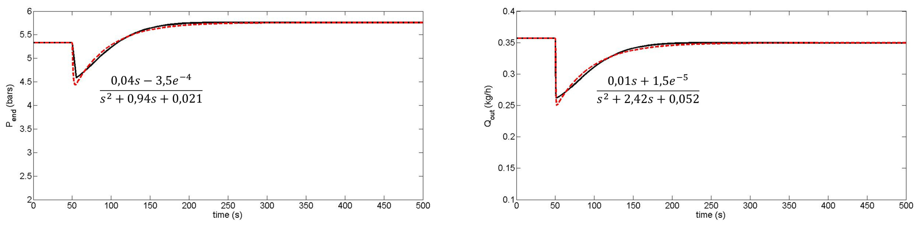
In the following, an illustrative example of the use of transfer function models is given. Using the responses to step changes in the screw rotation speed (Figure 20) and in the input flow rate (Figure 21), transfer functions describing the responses of the die pressure and the outlet flow rate are identified using the function “Ident” of the MATLAB identification toolbox. Results are shown in Figure 26 and Figure 27.
Second-order transfer functions plus delay are usually sufficient to get an acceptable fit of the input-output behavior. However, as mentioned above, the use of transfer functions is limited to a range of operating conditions where the assumption of linearity is satisfied. Moreover, black-box models only offer an input-output map of the system and no insight into the internal state.
8. Conclusion
Mathematical modeling of extrusion processes has led to essentially five types of models:
- explicit solutions of the mass balance equations, i.e., functions of time describing the residence time distribution;
- systems of differential equations, resulting from mass and energy balances expressed around a representation of the systems in the form of continuous-stirred reactors in series;
- systems of partial differential equations resulting from mass and energy (possibly momentum) balances in a distributed parameter representation of the system;
- PBM-DEM methods, including material properties in differential equation systems describing each particle characteristic evolutions using Newton’s second law of motion and the angular momentum
- black-box representations of the system, e.g., transfer functions or neural networks linking input and output operational variables, inferred from experimental data and using little or no a priori physical knowledge of the system.
The first class is essentially descriptive, and only the models in the second, third and last categories are of interest in terms of estimation and control. The second class of models can be seen as a first-order finite volume discretization of the partial differential equations involved in the third class of models. Changing the number of CSTRs directly influences both model formulation and the resolution of the solution profiles (numerical dispersion is influenced by the number of discretization cells and can be used in some way to represent physical dispersion). Distributed parameter models offer the advantage of uncoupling model formulation and the numerical solution technique. Any numerical schemes can be used, ranging from simple finite difference to sophisticated finite element or volume methods.
The PDE models can be complemented by ODEs representing the evolution of moving interfaces, and different models can be used for several sections of the process. The usual spatial representation is in the 1D axial direction, but could be extended to 2D or 3D representations, at the price of increased computational expense and less compatibility with model-based process control strategies, which exploit the simplicity of the model structure and/or sufficiently short computation times.
PBM-DEM methods classify particles with respect to their physical properties (such as granule size, moisture content, porosity, etc.). Differential equations obtained while applying PBM generally require the use of empirical or semi-empirical expressions, functions of particle mechanical characteristics (shear, velocities, etc) determined by DEM. The resulting detrimental effect of this particle-per-particle accurate description is a huge computational effort, inappropriate to control design.
Conversely, data-driven models can be very practical, since they are well-adapted to control frameworks. However, they do not exploit a priori knowledge and offer little insight into the process behavior, outside of the mere input-output dynamics.
To conclude, we primarily recommend a modeling approach based on distributed parameter models. The basic PDEs can be found in [38]. These equations together with boundary/continuity conditions can be used to represent several sections of an extruder with different screw configurations. Moreover, the kneading block behavior can be described using assumptions formulated in [55]. Finally, the PDEs can be completed by ODEs to determine the spatial extension of fully filled zones and their moving boundaries. The approach proposed in [159] can facilitate the computation. A global model scheme is shown in Figure 28.
Acknowledgments
This paper presents research results of the Belgian Network DYSCO (Dynamical Systems, Control and Optimization), funded by the Interuniversity Attraction Poles Programme, initiated by the Belgian State, Science Policy Office.
The authors acknowledge the support of the WBGreen MYCOMELTproject in the Convention No. 1217716, achieved in collaboration with the University of Liege (ULg). The scientific responsibility rests with its author(s).
Author Contributions
The authors contributed equally to the work.
Conflicts of Interest
The authors declare no conflict of interest.
References
- Gerrens, H. Handbuch der Technischen Polymerchemie. Von A. Echte. VCH Verlagsgesellschaft mbH, Weinheim 1993. 721 S., 398 Abb. und 57 Tab., geb., DM 276,–. Chem. Ing. Technik 1994, 66, 239. [Google Scholar] [CrossRef]
- Dover, H.W. Apparatus for Insulating or Covering Strands and Forming Same into Cables. U.S. Patent 699,459, 6 May 1902. [Google Scholar]
- DiNunzio, J.C.; Brough, C.; Hughey, J.R.; Miller, D.A.; Williams, R.O.; McGinity, J.W. Fusion production of solid dispersions containing a heat-sensitive active ingredient by hot melt extrusion and Kinetisol® dispersing. Eur. J. Pharm. Biopharm. 2010, 74, 340–351. [Google Scholar] [CrossRef] [PubMed]
- Crowley, M.M.; Zhang, F.; Repka, M.A.; Thumma, S.; Upadhye, S.B.; Kumar Battu, S.; McGinity, J.W.; Martin, C. Pharmaceutical applications of hot-melt extrusion: Part I. Drug Dev. Ind. Pharm. 2007, 33, 909–926. [Google Scholar] [CrossRef] [PubMed]
- Repka, M.A.; Battu, S.K.; Upadhye, S.B.; Thumma, S.; Crowley, M.M.; Zhang, F.; Martin, C.; McGinity, J.W. Pharmaceutical applications of hot-melt extrusion: Part II. Drug Dev. Ind. Pharm. 2007, 33, 1043–1057. [Google Scholar] [CrossRef] [PubMed]
- Hughey, J.R.; Keen, J.M.; Miller, D.A.; Kolter, K.; Langley, N.; McGinity, J.W. The use of inorganic salts to improve the dissolution characteristics of tablets containing Soluplus®-based solid dispersions. Eur. J. Pharm. Sci. 2013, 48, 758–766. [Google Scholar] [CrossRef] [PubMed]
- Thiry, J.; Krier, F.; Evrard, B. A review of pharmaceutical extrusion: Critical process parameters and scaling-up. Int. J. Pharm. 2015, 479, 227–240. [Google Scholar] [CrossRef] [PubMed]
- Harper, J.M.; Clark, J.P. Food extrusion. Crit. Rev. Food Sci. Nutr. 1979, 11, 155–215. [Google Scholar] [CrossRef]
- Van Zuilichem, D. Extrusion Cooking, Craft or Science? Ph.D. Thesis, Wageningen Agricultural University, Wageningen, 29 January 1992. [Google Scholar]
- Singh, S.; Gamlath, S.; Wakeling, L. Nutritional aspects of food extrusion: A review. Int. J. Food Sci. Technol. 2007, 42, 916–929. [Google Scholar] [CrossRef]
- Johnson, W.; Kudō, H. The Mechanics of Metal Extrusion; Manchester University Press: Manchester, England, 1962. [Google Scholar]
- Lee, E.; Mallett, R.; Yang, W.H. Stress and deformation analysis of the metal extrusion process. Computer Methods Appl. Mech. Eng. 1977, 10, 339–353. [Google Scholar] [CrossRef]
- Erisken, C.; Kalyon, D.M.; Wang, H. A hybrid twin screw extrusion/electrospinning method to process nanoparticle-incorporated electrospun nanofibres. Nanotechnology 2008, 19. [Google Scholar] [CrossRef] [PubMed]
- Ergun, A.; Yu, X.; Valdevit, A.; Ritter, A.; Kalyon, D.M. In vitro analysis and mechanical properties of twin screw extruded single-layered and coextruded multilayered poly (caprolactone) scaffolds seeded with human fetal osteoblasts for bone tissue engineering. J. Biomed. Mater. Res. Part A 2011, 99, 354–366. [Google Scholar] [CrossRef] [PubMed]
- Kalyon, D.; Yu, X.; Wang, H.; Valdevit, A.; Ritter, A. Twin Screw Extrusion Based Technologies Offer Novelty, Versatility, Reproducibility and Industrial Scalability for Fabrication of Tissue Engineering Scaffolds. J. Tissue Sci. Eng. 2013, 4. [Google Scholar] [CrossRef]
- Aktas, S.; Gevgilili, H.; Kucuk, I.; Sunol, A.; Kalyon, D.M. Extrusion of poly (ether imide) foams using pressurized CO2: Effects of imposition of supercritical conditions and nanosilica modifiers. Polym. Eng. Sci. 2014, 54, 2064–2074. [Google Scholar] [CrossRef]
- Saha, P.K. Aluminum Extrusion Technology; Asm International: Novelty, OH, USA, 2000. [Google Scholar]
- Hudson, R. Developments in the European Extrusion Industry; Rapra Technology Limited: Shrewsbury, England, 1995. [Google Scholar]
- Moreira, R.G.; Srivastava, A.K.; Gerrish, J.B. Feedforward control model for a twin-screw food extruder. Food Control 1990, 1, 179–184. [Google Scholar] [CrossRef]
- Singh, B.; Mulvaney, S.J. Modeling and process control of twin-screw cooking food extruders. J. Food Eng. 1994, 23, 403–428. [Google Scholar] [CrossRef]
- Schlosburg, J. Twin-Screw Food Extrusion: Control Case Study. Available online: http://homepages.rpi.edu/bequeb/URP/JoelS-presentation.pdf (accessed on 27 May 2016).
- Wang, L.; Smith, S.; Chessari, C. Continuous-time model predictive control of food extruder. Control Eng. Pract. 2008, 16, 1173–1183. [Google Scholar] [CrossRef]
- Trifkovic, M.; Sheikhzadeh, M.; Choo, K.; Rohani, S. Model predictive control of a twin-screw extruder for thermoplastic vulcanizate (TPV) applications. Comput. Chem. Eng. 2012, 36, 247–254. [Google Scholar] [CrossRef]
- Zhou, P.; Liu, H.; Tan, K.; Chen, C. Application and Research of Fuzzy Control Simulation in Twin Screw Extruder. Procedia Eng. 2012, 29, 542–546. [Google Scholar] [CrossRef]
- Kalyon, D.M.; Gotsis, A.D.; Yilmazer, U.; Gogos, C.G.; Sangani, H.; Aral, B.; Tsenoglou, C. Development of experimental techniques and simulation methods to analyze mixing in co-rotating twin screw extrusion. Adv. Polym. Technol. 1988, 8, 337–353. [Google Scholar] [CrossRef]
- Yilmazer, U.; Gogos, C.G.; Kalyon, D.M. Mat formation and unstable flows of highly filled suspensions in capillaries and continuous processors. Polym. Compos. 1989, 10, 242–248. [Google Scholar] [CrossRef]
- Kalyon, D.M.; Sangani, H.N. An experimental study of distributive mixing in fully intermeshing, co-rotating twin screw extruders. Polym. Eng. Sci. 1989, 29, 1018–1026. [Google Scholar] [CrossRef]
- Kalyon, D.; Jacob, C.; Yaras, P. An experimental study of the degree of fill and melt densification in fully-intermeshing, co-rotating twin screw extruders. Plast. Rubber Compos. Process. Appl. 1991, 16, 193–200. [Google Scholar]
- Kalyon, D.M.; Yazici, R.; Jacob, C.; Aral, B.; Sinton, S.W. Effects of air entrainment on the rheology of concentrated suspensions during continuous processing. Polym. Eng. Sci. 1991, 31, 1386–1392. [Google Scholar] [CrossRef]
- Kalyon, D.M.; Birinci, E.; Yazici, R.; Karuv, B.; Walsh, S. Electrical properties of composites as affected by the degree of mixedness of the conductive filler in the polymer matrix. Polym. Eng. Sci. 2002, 42, 1609–1617. [Google Scholar] [CrossRef]
- Lu, G.; Kalyon, D.M.; Yilgör, I.; Yilgör, E. Rheology and extrusion of medical-grade thermoplastic polyurethane. Polym. Eng. Sci. 2003, 43, 1863–1877. [Google Scholar] [CrossRef]
- Erol, M.; Kalyon, D. Assessment of the degree of mixedness of filled polymers: Effects of processing histories in batch mixer and co-rotating and counter-rotating twin screw extruders. Int. Polym. Proc. 2005, 20, 228–237. [Google Scholar] [CrossRef]
- Kalyon, D.M.; Dalwadi, D.; Erol, M.; Birinci, E.; Tsenoglu, C. Rheological behavior of concentrated suspensions as affected by the dynamics of the mixing process. Rheol. Acta 2006, 45, 641–658. [Google Scholar] [CrossRef]
- Kalyon, D.M.; Gevgilili, H.; Kowalczyk, J.E.; Prickett, S.E.; Murphy, C.M. Use of adjustable-gap on-line and off-line slit rheometers for the characterization of the wall slip and shear viscosity behavior of energetic formulations. J. Energetic Mater. 2006, 24, 175–193. [Google Scholar] [CrossRef]
- Choulak, S.; Couenne, F.; Le Gorrec, Y.; Jallut, C.; Cassagnau, P.; Michel, A. Generic dynamic model for simulation and control of reactive extrusion. Ind. Eng. Chem. Res. 2004, 43, 7373–7382. [Google Scholar] [CrossRef]
- Carneiro, O.S.; Covas, J.A.; Vergnes, B. Experimental and theoretical study of twin-screw extrusion of polypropylene. J. Appl. Polym. Sci. 2000, 78, 1419–1430. [Google Scholar] [CrossRef]
- Khalifeh, A.; Clermont, J.R. Numerical simulations of non-isothermal three-dimensional flows in an extruder by a finite-volume method. J. Non-Newton. Fluid Mech. 2005, 126, 7–22. [Google Scholar] [CrossRef]
- Kulshreshtha, M.; Zaror, C. An unsteady state model for twin screw extruders. Food Bioprod. Proc. Trans. Inst. Chem. Eng. Part C 1992, 70, 21–28. [Google Scholar]
- Kumar, A.; Ganjyal, G.M.; Jones, D.D.; Hanna, M.A. Digital image processing for measurement of residence time distribution in a laboratory extruder. J. Food Eng. 2006, 75, 237–244. [Google Scholar] [CrossRef]
- Altomare, R.E.; Ghossi, P. An analysis of residence time distribution patterns in a twin screw cooking extruder. Biotechnol. Prog. 1986, 2, 157–163. [Google Scholar] [CrossRef] [PubMed]
- Mange, C.; Boissonnat, P.; Gelus, M. Distribution of residence times and comparison of three twin-screw extruders of different size. In Extrusion Technology for the Food Industry; O’Connor, C., Ed.; Elsevier Applied Sciences: London, England, 1987; pp. 117–131. [Google Scholar]
- Danckwerts, P. Continuous flow systems: Distribution of residence times. Chem. Eng. Sci. 1953, 2, 1–13. [Google Scholar] [CrossRef]
- Brenner, H. The diffusion model of longitudinal mixing in beds of finite length. Numerical values. Chem. Eng. Sci. 1962, 17, 229–243. [Google Scholar] [CrossRef]
- Levenspiel, O. Chemical reaction engineering. Ind. Eng. Chem. Res. 1999, 38, 4140–4143. [Google Scholar] [CrossRef]
- Kumar, A.; Vercruysse, J.; Vanhoorne, V.; Toiviainen, M.; Panouillot, P.E.; Juuti, M.; Vervaet, C.; Remon, J.P.; Gernaey, K.V.; De Beer, T.; et al. Conceptual framework for model-based analysis of residence time distribution in twin-screw granulation. Eur. J. Pharm. Sci. 2015, 71, 25–34. [Google Scholar] [CrossRef] [PubMed]
- Ziegler, G.R.; Aguilar, C.A. Residence time distribution in a co-rotating, twin-screw continuous mixer by the step change method. J. Food Eng. 2003, 59, 161–167. [Google Scholar] [CrossRef]
- Poulesquen, A.; Vergnes, B. A study of residence time distribution in co-rotating twin-screw extruders. Part I: Theoretical modeling. Polym. Eng. Sci. 2003, 43, 1841–1848. [Google Scholar] [CrossRef]
- Poulesquen, A.; Vergnes, B.; Cassagnau, P.; Michel, A.; Carneiro, O.S.; Covas, J.A. A study of residence time distribution in co-rotating twin-screw extruders. Part II: Experimental validation. Polym. Eng. Sci. 2003, 43, 1849–1862. [Google Scholar] [CrossRef]
- De Ruyck, H. Modelling of the residence time distribution in a twin screw extruder. J. Food Eng. 1997, 32, 375–390. [Google Scholar] [CrossRef]
- Puaux, J.; Bozga, G.; Ainser, A. Residence time distribution in a corotating twin-screw extruder. Chem. Eng. Sci. 2000, 55, 1641–1651. [Google Scholar] [CrossRef]
- Kumar, A.; Ganjyal, G.M.; Jones, D.D.; Hanna, M.A. Modeling residence time distribution in a twin-screw extruder as a series of ideal steady-state flow reactors. J. Food Eng. 2008, 84, 441–448. [Google Scholar] [CrossRef]
- Elsey, J.R. Dynamic Modelling, Measurement and Control of Co-rotating Twin-Screw Extruders. Ph.D. Thesis, University of Sydney, Sydney, Australia, 25 August 2002. [Google Scholar]
- Choulak, S.E. Modélisation et Commande d’un Procédé D’extrusion Réactive. Ph.D. Thesis, Université Claude Bernard-Lyon I, Lyon, France, 2004. [Google Scholar]
- De Ville d’Avray, M.A.; Isambert, A.; Brochot, S. Development of a global mathematical model for reactive extrusion processes in corotating twin-screw extruders. Comput. Aided Chem. Eng. 2010, 28, 769–774. [Google Scholar]
- Eitzlmayr, A.; Koscher, G.; Reynolds, G.; Huang, Z.; Booth, J.; Shering, P.; Khinast, J. Mechanistic modeling of modular co-rotating twin-screw extruders. Int. J. Pharm. 2014, 474, 157–176. [Google Scholar] [CrossRef] [PubMed]
- Ganzeveld, K.; Capel, J.; Van Der Wal, D.; Janssen, L. The modelling of counter-rotating twin screw extruders as reactors for single-component reactions. Chem. Eng. Sci. 1994, 49, 1639–1649. [Google Scholar] [CrossRef]
- De Graaf, R.; Rohde, M.; Janssen, L. A novel model predicting the residence-time distribution during reactive extrusion. Chem. Eng. Sci. 1997, 52, 4345–4356. [Google Scholar] [CrossRef]
- Goma-Bilongo, T.; Couenne, F.; Jallut, C.; Le Gorrec, Y.; Di Martino, A. Dynamic Modeling of the Reactive Twin-Screw Corotating Extrusion Process: Experimental Validation by Using Inlet Glass Fibers Injection Response and Application to Polymers Degassing. Ind. Eng. Chem. Res. 2012, 51, 11381–11388. [Google Scholar] [CrossRef] [Green Version]
- Janssen, L. Twin Screw Extrusion; Elsevier Scientific Publishing Company: Amsterdam, Netherlands, 1978. [Google Scholar]
- Booy, M. Isothermal flow of viscous liquids in corotating twin screw devices. Polym. Eng. Sci. 1980, 20, 1220–1228. [Google Scholar] [CrossRef]
- Goffart, D.; Van der Wal, D.; Klomp, E.; Hoogstraten, H.; Janssen, L.; Breysse, L.; Trolez, Y. Three-dimensional flow modeling of a self-wiping corotating twin-screw extruder. Part I: The transporting section. Polym. Eng. Sci. 1996, 36, 901–911. [Google Scholar] [CrossRef]
- Van Der Wal, D.; Goffart, D.; Klomp, E.; Hoogstraten, H.; Janssen, L. Three-dimensional flow modeling of a self-wiping corotating twin-screw extruder. Part II: The kneading section. Polym. Eng. Sci. 1996, 36, 912–924. [Google Scholar] [CrossRef]
- Cheng, H.; Manas-Zloczower, I. Distributive mixing in conveying elements of a ZSK-53 co-rotating twin screw extruder. Polym. Eng. Sci. 1998, 38, 926–935. [Google Scholar] [CrossRef]
- Ishikawa, T.; Kihara, S.i.; Funatsu, K. 3-D non-isothermal flow field analysis and mixing performance evaluation of kneading blocks in a co-rotating twin srew extruder. Polym. Eng. Sci. 2001, 41, 840–849. [Google Scholar] [CrossRef]
- Potente, H.; Többen, W.H. Improved Design of Shearing Sections with New Calculation Models Based on 3D Finite-Element Simulations. Macromol. Mater. Eng. 2002, 287, 808–814. [Google Scholar] [CrossRef]
- Bertrand, F.; Thibault, F.; Delamare, L.; Tanguy, P.A. Adaptive finite element simulations of fluid flow in twin-screw extruders. Comput. Chem. Eng. 2003, 27, 491–500. [Google Scholar] [CrossRef]
- Ficarella, A.; Milanese, M.; Laforgia, D. Numerical study of the extrusion process in cereals production: Part I. Fluid-dynamic analysis of the extrusion system. J. Food Eng. 2006, 73, 103–111. [Google Scholar] [CrossRef]
- Malik, M.; Kalyon, D. 3d finite element simulation of processing of generalized newtonian fluids in counter-rotating and tangential tse and die combination. Int. Polym. Proc. 2005, 20, 398–409. [Google Scholar] [CrossRef]
- Kalyon, D.; Malik, M. An integrated approach for numerical analysis of coupled flow and heat transfer in co-rotating twin screw extruders. Int. Polym. Proc. 2007, 22, 293–302. [Google Scholar] [CrossRef]
- Barrera, M.; Vega, J.; Martínez-Salazar, J. Three-dimensional modelling of flow curves in co-rotating twin-screw extruder elements. J. Mater. Proc. Technol. 2008, 197, 221–224. [Google Scholar] [CrossRef]
- Rodríguez, E.O. Numerical Simulations of Reactive Extrusion in Twin Screw Extruders. Ph.D. Thesis, University of Waterloo, Waterloo, ON, Canada, 18 January 2009. [Google Scholar]
- Sarhangi Fard, A.; Hulsen, M.A.; Meijer, H.E.; Famili, N.M.; Anderson, P.D. Tools to Simulate Distributive Mixing in Twin-Screw Extruders. Macromol. Theory Simul. 2012, 21, 217–240. [Google Scholar] [CrossRef]
- Fard, A.S.; Anderson, P.D. Simulation of distributive mixing inside mixing elements of co-rotating twin-screw extruders. Comput. Fluids 2013, 87, 79–91. [Google Scholar] [CrossRef]
- Hétu, J.F.; Ilinca, F. Immersed boundary finite elements for 3D flow simulations in twin-screw extruders. Comput. Fluids 2013, 87, 2–11. [Google Scholar] [CrossRef]
- Rathod, M.L.; Kokini, J.L. Effect of mixer geometry and operating conditions on mixing efficiency of a non-Newtonian fluid in a twin screw mixer. J. Food Eng. 2013, 118, 256–265. [Google Scholar] [CrossRef]
- Djoudi, H.; Gelin, J.; Barrière, T. Simulation numérique par éléments finis de l écoulement dans un mélangeur bi-vis et l interaction mélange-mélangeur. 11e Colloque National en Calcul des Structures. 2013. Available online: http://csma2013.csma.fr/resumes/rN47U19K8.pdf (accessed on 27 May 2016).
- Carneiro, O.; Nóbrega, J.; Pinho, F.; Oliveira, P. Computer aided rheological design of extrusion dies for profiles. J. Mater. Proc. Technol. 2001, 114, 75–86. [Google Scholar] [CrossRef]
- Lin, Z.; Juchen, X.; Xinyun, W.; Guoan, H. Optimization of die profile for improving die life in the hot extrusion process. J. Mater. Proc. Technol. 2003, 142, 659–664. [Google Scholar] [CrossRef]
- Patil, P.D.; Feng, J.J.; Hatzikiriakos, S.G. Constitutive modeling and flow simulation of polytetrafluoroethylene (PTFE) paste extrusion. J. Non-Newton. Fluid Mech. 2006, 139, 44–53. [Google Scholar] [CrossRef]
- Mitsoulis, E.; Hatzikiriakos, S.G. Steady flow simulations of compressible PTFE paste extrusion under severe wall slip. J. Non-Newton. Fluid Mech. 2009, 157, 26–33. [Google Scholar] [CrossRef]
- Radl, S.; Tritthart, T.; Khinast, J.G. A novel design for hot-melt extrusion pelletizers. Chem. Eng. Sci. 2010, 65, 1976–1988. [Google Scholar] [CrossRef]
- Ardakani, H.A.; Mitsoulis, E.; Hatzikiriakos, S.G. Thixotropic flow of toothpaste through extrusion dies. J. Non-Newton. Fluid Mech. 2011, 166, 1262–1271. [Google Scholar] [CrossRef]
- Lawal, A.; Railkar, S.; Kalyon, D.M. Mathematical modeling of three-dimensional die flows of viscoplastic fluids with wall slip. J. Reinf. Plast. Compos. 2000, 19, 1483–1492. [Google Scholar] [CrossRef]
- Kalyon, D.M.; Gevgilili, H. Wall slip and extrudate distortion of three polymer melts. J. Rheol. (1978-present) 2003, 47, 683–699. [Google Scholar] [CrossRef]
- Kalyon, D.M. Apparent slip and viscoplasticity of concentrated suspensions. J. Rheol. (1978-present) 2005, 49, 621–640. [Google Scholar] [CrossRef]
- Birinci, E.; Kalyon, D.M. Development of extrudate distortions in poly (dimethyl siloxane) and its suspensions with rigid particles. J. Rheol. (1978-present) 2006, 50, 313–326. [Google Scholar] [CrossRef]
- Kalyon, D.M. An analytical model for steady coextrusion of viscoplastic fluids in thin slit dies with wall slip. Polym. Eng. Sci. 2010, 50, 652–664. [Google Scholar] [CrossRef]
- Tang, H.; Kalyon, D.M. Unsteady circular tube flow of compressible polymeric liquids subject to pressure-dependent wall slip. J. Rheol. (1978-present) 2008, 52, 507–525. [Google Scholar] [CrossRef]
- Tang, H.; Kalyon, D.M. Time-dependent tube flow of compressible suspensions subject to pressure dependent wall slip: Ramifications on development of flow instabilities. J. Rheol. (1978-present) 2008, 52, 1069–1090. [Google Scholar] [CrossRef]
- Lawal, A.; Kalyon, D.M.; Ji, Z. Computational study of chaotic mixing in co-rotating two-tipped kneading paddles: Two-dimensional approach. Polym. Eng. Sci. 1993, 33, 140–148. [Google Scholar] [CrossRef]
- Lawal, A.; Kalyon, D.M. Mechanisms of mixing in single and co-rotating twin screw extruders. Polym. Eng. Sci. 1995, 35, 1325–1338. [Google Scholar] [CrossRef]
- Lawal, A.; Kalyon, D. Three Dimensional Analysis of Co-rotating Twin Screw Extrusion Using Tools of Dynamics. In Technical Papers of the Annual Technical Conference-Society of Plastics Engineers Incorporated; Society of plastics engineers Inc.: Bethel, AK, USA, 1993; p. 3397. [Google Scholar]
- Zhu, L.; Narh, K.A.; Hyun, K.S. Evaluation of numerical simulation methods in reactive extrusion. Adv. Polym. Technol. 2005, 24, 183–193. [Google Scholar] [CrossRef]
- Werner, H.P. Das Betriebsverhalten der zweiwelligen Knetscheiben-Schneckenpresse vom Typ ZSK bei der Verarbeitung von hochviskosen Flüssigkeiten: Ein Beitrag zur Theorie und Praxis der ZSK. Ph.D. Thesis, Technische Universität München, Munich, Germany, 1976. [Google Scholar]
- Yacu, W. Modeling a twin screw co-rotating extruder. J. Food Process Eng. 1985, 8, 1–21. [Google Scholar] [CrossRef]
- Meijer, H.; Elemans, P. The modeling of continuous mixers. Part I: The corotating twin-screw extruder. Polym. Eng. Sci. 1988, 28, 275–290. [Google Scholar] [CrossRef]
- Tayeb, J.; Vergnes, B.; Valle, G.D. Theoretical computation of the isothermal flow through the reverse screw element of a twin screw extrusion cooker. J. Food Sci. 1988, 53, 616–625. [Google Scholar] [CrossRef]
- Tayeb, J.; Vergnes, B.; Valle, G.D. A basic model for a twin-screw extruder. J. Food Sci. 1989, 54, 1047–1056. [Google Scholar] [CrossRef]
- Della Valle, G.; Barres, C.; Plewa, J.; Tayeb, J.; Vergnes, B. Computer simulation of starchy products’ transformation by twin-screw extrusion. J. Food Eng. 1993, 19, 1–31. [Google Scholar] [CrossRef]
- White, J.L.; Chen, Z. Simulation of non-isothermal flow in modular co-rotating twin screw extrusion. Polym. Eng. Sci. 1994, 34, 229–237. [Google Scholar] [CrossRef]
- Michaeli, W.; Grefenstein, A. An analytical model of the conveying behaviour of closely intermeshing co-rotating twin screw extruders. Int. Polym. Process. 1996, 11, 121–128. [Google Scholar] [CrossRef]
- Vergnes, B.; Valle, G.D.; Delamare, L. A global computer software for polymer flows in corotating twin screw extruders. Polym. Eng. Sci. 1998, 38, 1781–1792. [Google Scholar] [CrossRef]
- Kulshreshtha, M.; Jukes, D.; Zaror, C. Generalized steady state model for twin screw extruders. Food Bioprod. Process. 1991, 69, 189–199. [Google Scholar]
- Martelli, F.G. Twin-Screw Extruders: A Basic Understanding; Van Nostrand Reinhold Company: New York, NY, USA, 1983. [Google Scholar]
- Li, C.H. Modelling extrusion cooking. Math. Comput. Model. 2001, 33, 553–563. [Google Scholar] [CrossRef]
- Diagne, M.; Dos Santos Martins, V.; Couenne, F.; Maschke, B.; Jallut, C. Modélisation d’un procédé d’extrusion par deux systèmes d’équations d’évolution couplés par une interface mobile. J. Eur. des Syst. Autom. 2011, 45, 665–691. [Google Scholar]
- Vande Wouwer, A.; Saucez, P.; Vilas, C. Simulation of Ode/Pde Models with MATLAB®, OCTAVE and SCILAB: Scientific and Engineering Applications; Springer International Publishing: Cham, Switzerland, 2014. [Google Scholar]
- Ramkrishna, D. Population Balances: Theory and Applications to Particulate Systems in Engineering; Academic Press: London, UK, 2000. [Google Scholar]
- Iveson, S.; Litster, J.; Ennis, B. Fundamental studies of granule consolidation Part 1: Effects of binder content and binder viscosity. Powder Technol. 1996, 88, 15–20. [Google Scholar] [CrossRef]
- Hounslow, M.; Pearson, J.; Instone, T. Tracer studies of high-shear granulation: II. Population balance modeling. AIChE J. 2001, 47, 1984–1999. [Google Scholar] [CrossRef]
- Darelius, A.; Brage, H.; Rasmuson, A.; Björn, I.N.; Folestad, S. A volume-based multi-dimensional population balance approach for modelling high shear granulation. Chem. Eng. Sci. 2006, 61, 2482–2493. [Google Scholar] [CrossRef]
- Poon, J.M.H.; Ramachandran, R.; Sanders, C.F.; Glaser, T.; Immanuel, C.D.; Doyle, F.J., III; Litster, J.D.; Stepanek, F.; Wang, F.Y.; Cameron, I.T. Experimental validation studies on a multi-dimensional and multi-scale population balance model of batch granulation. Chem. Eng. Sci. 2009, 64, 775–786. [Google Scholar] [CrossRef]
- Gerstlauer, A.; Motz, S.; Mitrović, A.; Gilles, E.D. Development, analysis and validation of population models for continuous and batch crystallizers. Chem. Eng. Sci. 2002, 57, 4311–4327. [Google Scholar] [CrossRef]
- Sen, M.; Ramachandran, R. A multi-dimensional population balance model approach to continuous powder mixing processes. Adv. Powder Technol. 2013, 24, 51–59. [Google Scholar] [CrossRef]
- Bilgili, E.; Scarlett, B. Population balance modeling of non-linear effects in milling processes. Powder Technol. 2005, 153, 59–71. [Google Scholar] [CrossRef]
- Verkoeijen, D.; Pouw, G.A.; Meesters, G.M.; Scarlett, B. Population balances for particulate processes—A volume approach. Chem. Eng. Sci. 2002, 57, 2287–2303. [Google Scholar] [CrossRef]
- Cameron, I.; Wang, F.; Immanuel, C.; Stepanek, F. Process systems modelling and applications in granulation: A review. Chem. Eng. Sci. 2005, 60, 3723–3750. [Google Scholar] [CrossRef]
- Sen, M. Multiscale Modeling and Validation of Particulate Processes. Ph.D. Thesis, Rutgers University-Graduate School-New Brunswick, New Brunswick, NJ, USA, May 2015. [Google Scholar]
- Kumar, A. Experimental and model-based analysis of twin-screw wet granulation in pharmaceutical processes. Ph.D. Thesis, Ghent University, Ghent, Belgium, 14 October 2015. [Google Scholar]
- Barrasso, D.; Walia, S.; Ramachandran, R. Multi-component population balance modeling of continuous granulation processes: A parametric study and comparison with experimental trends. Powder Technol. 2013, 241, 85–97. [Google Scholar] [CrossRef]
- Barrasso, D.; Eppinger, T.; Pereira, F.E.; Aglave, R.; Debus, K.; Bermingham, S.K.; Ramachandran, R. A multi-scale, mechanistic model of a wet granulation process using a novel bi-directional PBM–DEM coupling algorithm. Chem. Eng. Sci. 2015, 123, 500–513. [Google Scholar] [CrossRef]
- Gantt, J.A.; Gatzke, E.P. High-shear granulation modeling using a discrete element simulation approach. Powder Technol. 2005, 156, 195–212. [Google Scholar] [CrossRef]
- Zhu, H.; Zhou, Z.; Yang, R.; Yu, A. Discrete particle simulation of particulate systems: A review of major applications and findings. Chem. Eng. Sci. 2008, 63, 5728–5770. [Google Scholar] [CrossRef]
- Ketterhagen, W.R.; am Ende, M.T.; Hancock, B.C. Process modeling in the pharmaceutical industry using the discrete element method. J. Pharm. Sci. 2009, 98, 442–470. [Google Scholar] [CrossRef] [PubMed]
- Liu, P.; Yang, R.; Yu, A. DEM study of the transverse mixing of wet particles in rotating drums. Chem. Eng. Sci. 2013, 86, 99–107. [Google Scholar] [CrossRef]
- Herrmann, H.; Luding, S. Modeling granular media on the computer. Contin. Mech. Thermodyn. 1998, 10, 189–231. [Google Scholar] [CrossRef]
- Cundall, P.A.; Strack, O.D. A discrete numerical model for granular assemblies. Geotechnique 1979, 29, 47–65. [Google Scholar] [CrossRef]
- Moysey, P.; Thompson, M. Modelling the solids inflow and solids conveying of single-screw extruders using the discrete element method. Powder Technol. 2005, 153, 95–107. [Google Scholar] [CrossRef]
- Yang, R.; Zou, R.; Yu, A. Microdynamic analysis of particle flow in a horizontal rotating drum. Powder Technol. 2003, 130, 138–146. [Google Scholar] [CrossRef]
- Hassanpour, A.; Tan, H.; Bayly, A.; Gopalkrishnan, P.; Ng, B.; Ghadiri, M. Analysis of particle motion in a paddle mixer using Discrete Element Method (DEM). Powder Technol. 2011, 206, 189–194. [Google Scholar] [CrossRef]
- Wang, M.; Yang, R.; Yu, A. DEM investigation of energy distribution and particle breakage in tumbling ball mills. Powder Technol. 2012, 223, 83–91. [Google Scholar] [CrossRef]
- Kumar, A.; Gernaey, K.V.; De Beer, T.; Nopens, I. Model-based analysis of high shear wet granulation from batch to continuous processes in pharmaceutical production–a critical review. Eur. J. Pharm. Biopharm. 2013, 85, 814–832. [Google Scholar] [CrossRef] [PubMed] [Green Version]
- Barrasso, D. Multi-scale modeling of wet granulation processes. Ph.D. Thesis, Rutgers University-Graduate School-New Brunswick, New Brunswick, NJ, USA, October 2015. [Google Scholar]
- Kumar, A.; Vercruysse, J.; Mortier, S.T.; Vervaet, C.; Remon, J.P.; Gernaey, K.V.; De Beer, T.; Nopens, I. Model-based analysis of a twin-screw wet granulation system for continuous solid dosage manufacturing. Comput. Chem. Eng. 2016, 89, 62–70. [Google Scholar] [CrossRef] [Green Version]
- Kulju, T.; Paavola, M.; Spittka, H.; Keiski, R.L.; Juuso, E.; Leiviskä, K.; Muurinen, E. Modeling continuous high-shear wet granulation with DEM-PB. Chem. Eng. Sci. 2016, 142, 190–200. [Google Scholar] [CrossRef]
- Ramachandran, R. Integrated PBM-DEM Model Of A Continuous Granulation Process; Department of Chemical and Biochemical Engineering Rutgers University: Piscataway, NJ, USA, 2016. Available online: http://www.star-global-conference.com/sites/default/files/publicpdfpresentation/SGC2016RutgersUniversityRohitRamachandran.pdf (accessed on 27 May 2016).
- Rajniak, P.; Stepanek, F.; Dhanasekharan, K.; Fan, R.; Mancinelli, C.; Chern, R. A combined experimental and computational study of wet granulation in a Wurster fluid bed granulator. Powder Technol. 2009, 189, 190–201. [Google Scholar] [CrossRef]
- Fries, L.; Antonyuk, S.; Heinrich, S.; Palzer, S. DEM–CFD modeling of a fluidized bed spray granulator. Chem. Eng. Sci. 2011, 66, 2340–2355. [Google Scholar] [CrossRef]
- Sen, M.; Barrasso, D.; Singh, R.; Ramachandran, R. A multi-scale hybrid CFD-DEM-PBM description of a fluid-bed granulation process. Processes 2014, 2, 89–111. [Google Scholar] [CrossRef]
- Seborg, D.E.; Mellichamp, D.A.; Edgar, T.F.; Doyle, F.J., III. Process Dynamics and Control; John Wiley & Sons: Hoboken, NJ, USA, 2010. [Google Scholar]
- Hassan, G.; Parnaby, J. Model reference optimal steady-state adaptive computer control of plastics extrusion processes. Polym. Eng. Sci. 1981, 21, 276–284. [Google Scholar] [CrossRef]
- Costin, M.; Taylor, P.; Wright, J. On the dynamics and control of a plasticating extruder. Polym. Eng. Sci. 1982, 22, 1095–1106. [Google Scholar] [CrossRef]
- Chan, D.; Nelson, R.; Lee, L.J. Dynamic behavior of a single screw plasticating extruder part II: Dynamic modeling. Polym. Eng. Sci. 1986, 26, 152–161. [Google Scholar] [CrossRef]
- Lu, Q.; Mulvaney, S.; Hsieh, F.; Huff, H. Model and strategies for computer control of a twin-screw extruder. Food Control 1993, 4, 25–33. [Google Scholar] [CrossRef]
- Cayot, N.; Bounie, D.; Baussart, H. Dynamic modelling for a twin screw food extruder: Analysis of the dynamic behaviour through process variables. J. Food Eng. 1995, 25, 245–260. [Google Scholar] [CrossRef]
- Haley, T.A.; Mulvaney, S.J. On-line system identification and control design of an extrusion cooking process: Part I. System identification. Food Control 2000, 11, 103–120. [Google Scholar] [CrossRef]
- Rosenblatt, F. The perceptron: A probabilistic model for information storage and organization in the brain. Psychol. Rev. 1958, 65, 386–408. [Google Scholar] [CrossRef] [PubMed]
- Werbos, P. Beyond Regression: New Tools for Prediction and Analysis in the Behavioral Sciences. Ph.D. Thesis, Harvard University, Cambridge, MA, USA, 1974. [Google Scholar]
- Minsky, M.; Papert, S. Perceptrons: An Introduction to Computational Geometry, expanded ed.; MIT Press: Cambridge, MA, USA, 1988. [Google Scholar]
- Vande Wouwer, A.; Renotte, C.; Bogaerts, P. Biological reaction modeling using radial basis function networks. Comput. Chem. Eng. 2004, 28, 2157–2164. [Google Scholar] [CrossRef]
- Morgan, N.; Bourlard, H. Neural networks for statistical recognition of continuous speech. Proc. IEEE 1995, 83, 742–772. [Google Scholar] [CrossRef]
- Gosselin, B. Multilayer perceptrons combination applied to handwritten character recognition. Neural Proc. Lett. 1996, 3, 3–10. [Google Scholar] [CrossRef]
- Willis, M.J.; Montague, G.A.; Di Massimo, C.; Tham, M.T.; Morris, A. Artificial neural networks in process estimation and control. Automatica 1992, 28, 1181–1187. [Google Scholar] [CrossRef]
- Chiu, S. Developing commercial applications of intelligent control. Control Syst. IEEE 1997, 17, 94–100. [Google Scholar] [CrossRef]
- Linko, P.; Uemura, K.; Zhu, Y.; Ferikainen, T. Application of neural network models in fuzzy extrusion control. Food Bioprod. Proc. Trans. Inst. Chem. Eng. Part C 1992, 70, 131–137. [Google Scholar]
- Eerikäinen, T.; Zhu, Y.H.; Linko, P. Neural networks in extrusion process identification and control. Food Control 1994, 5, 111–119. [Google Scholar] [CrossRef]
- Popescu, O.; Popescu, D.C.; Wilder, J.; Karwe, M.V. A new approach to modeling and control of a food extrusion process using artificial neural network and an expert system. J. Food Process Eng. 2001, 24, 17–36. [Google Scholar] [CrossRef]
- Ganjyal, G.; Hanna, M.; Jones, D. Modeling Selected Properties of Extruded Waxy Maize Cross-Linked Starches with Neural Networks. J. Food Sci. 2003, 68, 1384–1388. [Google Scholar] [CrossRef]
- Kim, E.K.; White, J.L. Isothermal transient startup of a starved flow modular co-rotating twin screw extruder. Polym. Eng. Sci. 2000, 40, 543–553. [Google Scholar] [CrossRef]
Figure 1.
Sketch of a simple extruder: variable definition.

Figure 2.
A simple case study.
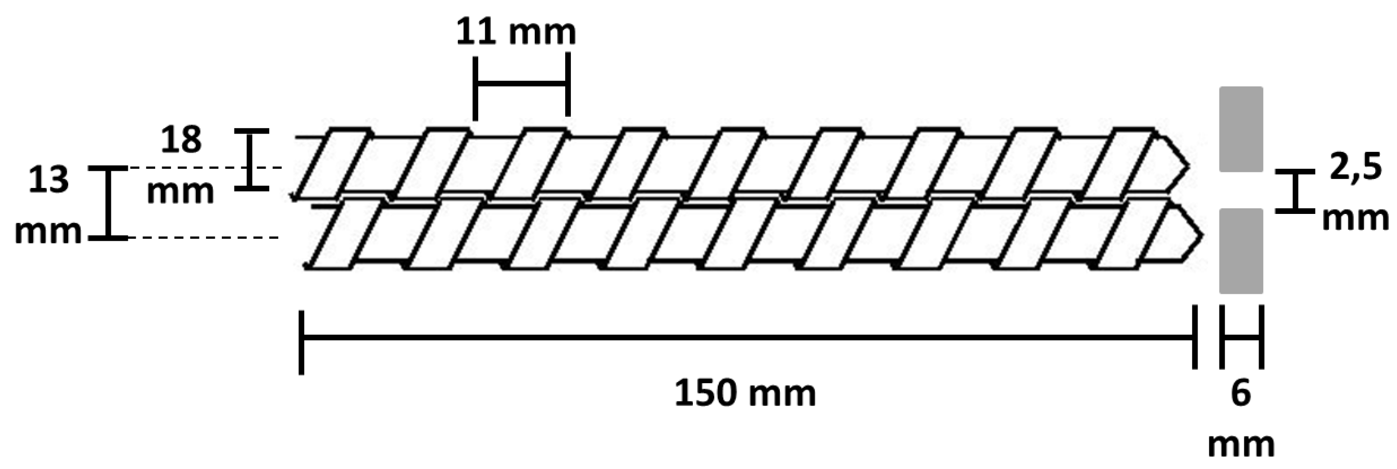
Figure 3.
Measurement of the residence time distribution (RTD) at RPM and kg/h.

Figure 4.
Plug flow reactor, continuous stirred tank reactor and actual reactor residence time distributions.
Figure 4.
Plug flow reactor, continuous stirred tank reactor and actual reactor residence time distributions.
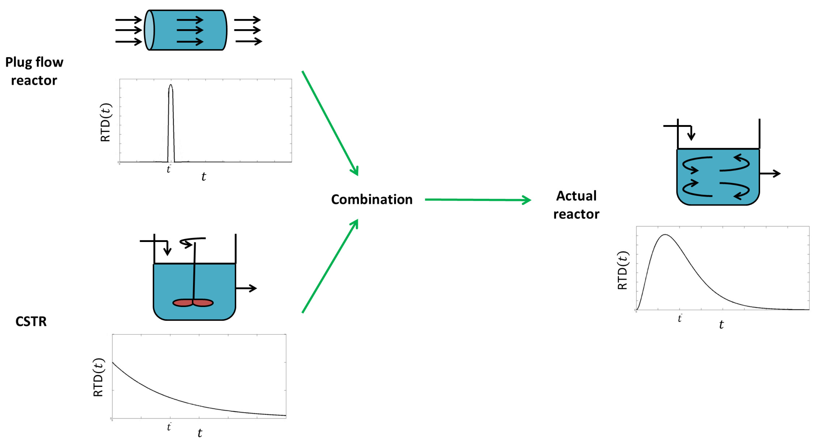
Figure 5.
Modeling of the residence time distribution through cascades of continuous stirred-tank reactors (CSTRs) or cascades of plug-flow reactor and CSTRs.
Figure 5.
Modeling of the residence time distribution through cascades of continuous stirred-tank reactors (CSTRs) or cascades of plug-flow reactor and CSTRs.
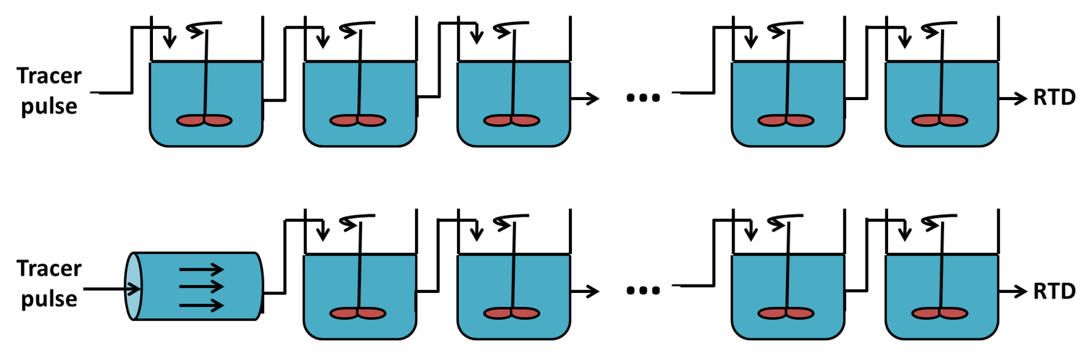
Figure 6.
Discretization of the extrusion device in volume elements, subdivided in cascades of ideal CSTRs.
Figure 6.
Discretization of the extrusion device in volume elements, subdivided in cascades of ideal CSTRs.
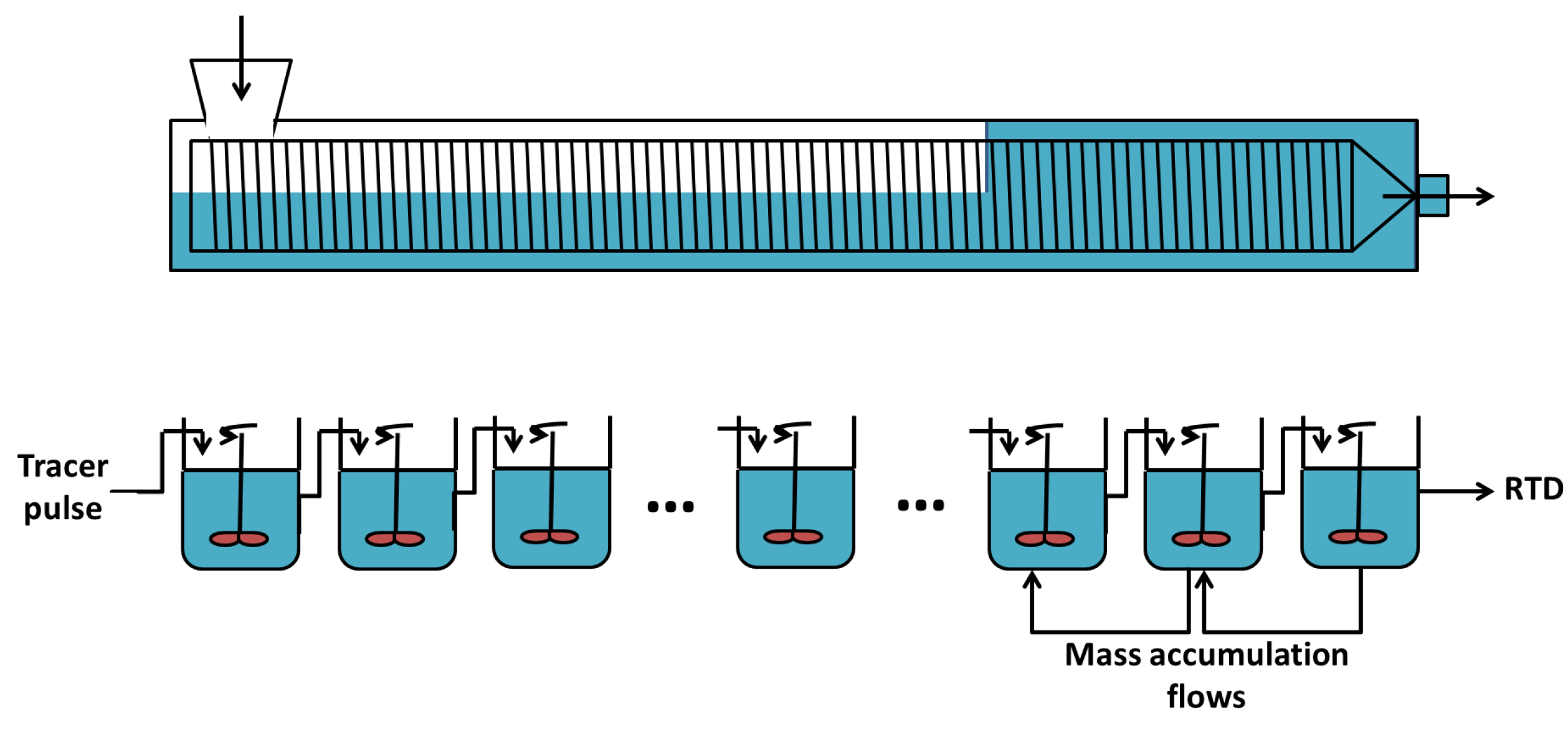
Figure 7.
Plug flow reactor and cascade of CSTRs with forward and backward flows.
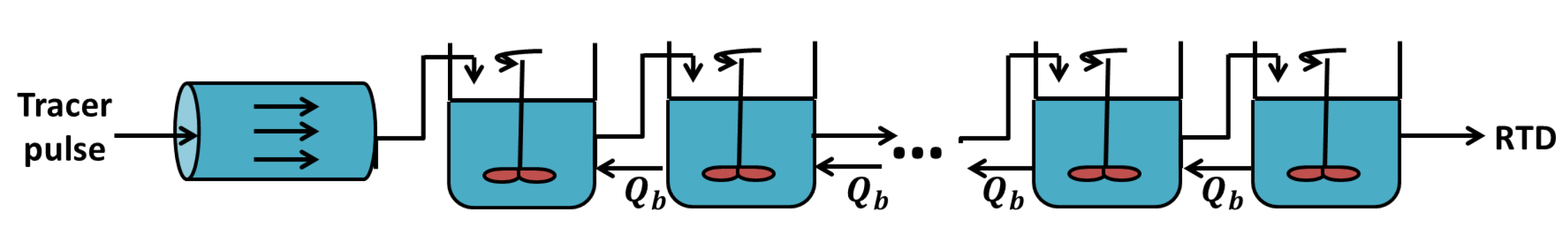
Figure 8.
Plug flow reactor in series with a cascade of CSTRs with dead zones.
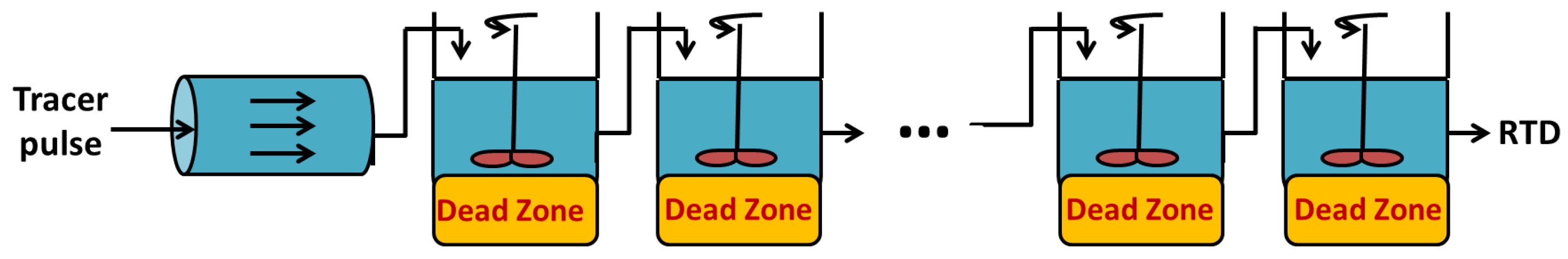
Figure 9.
RTD model validation. Solid line: model prediction; dashed line: experimental data.
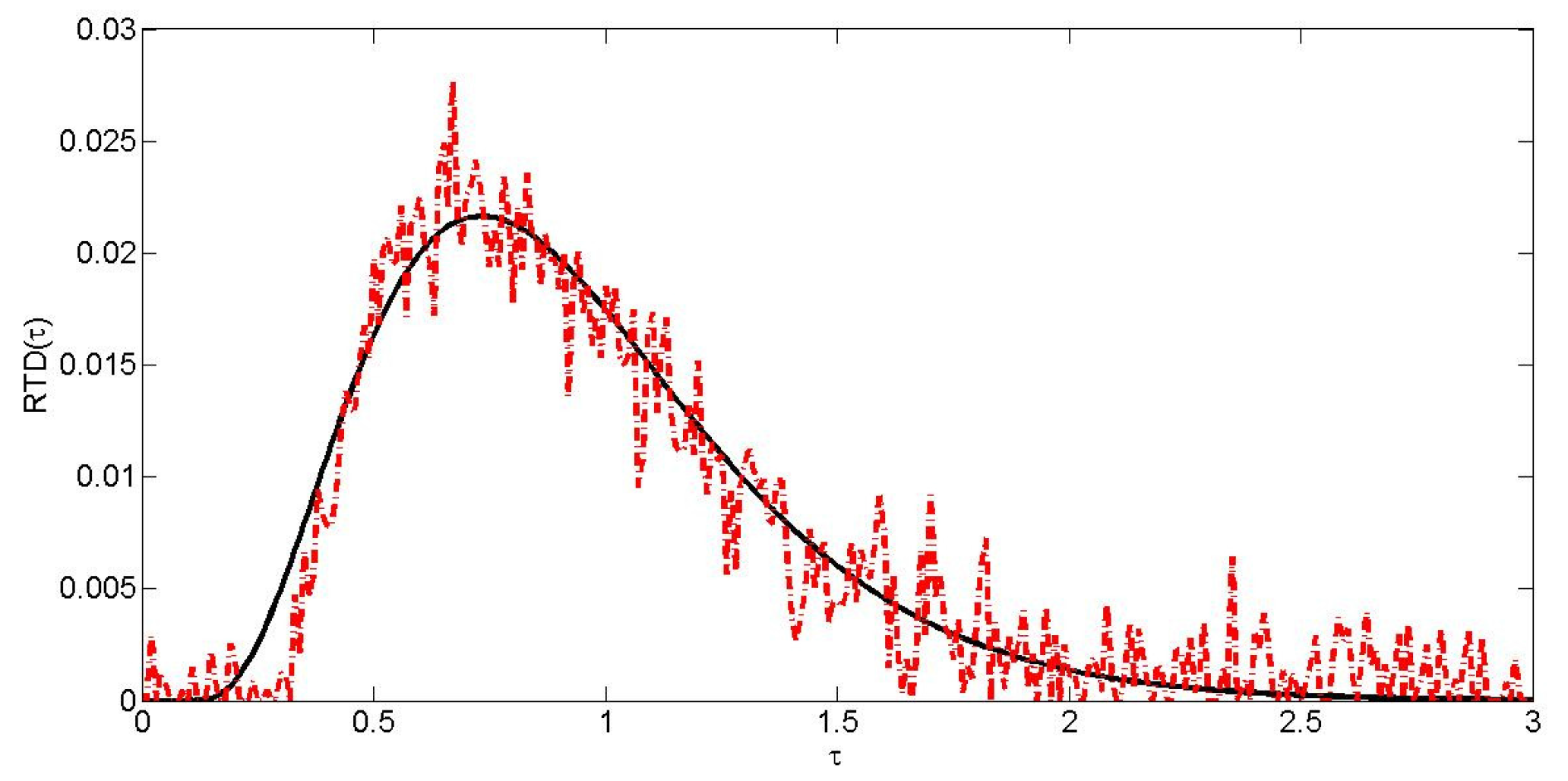
Figure 10.
Geometry of a C-chamber.
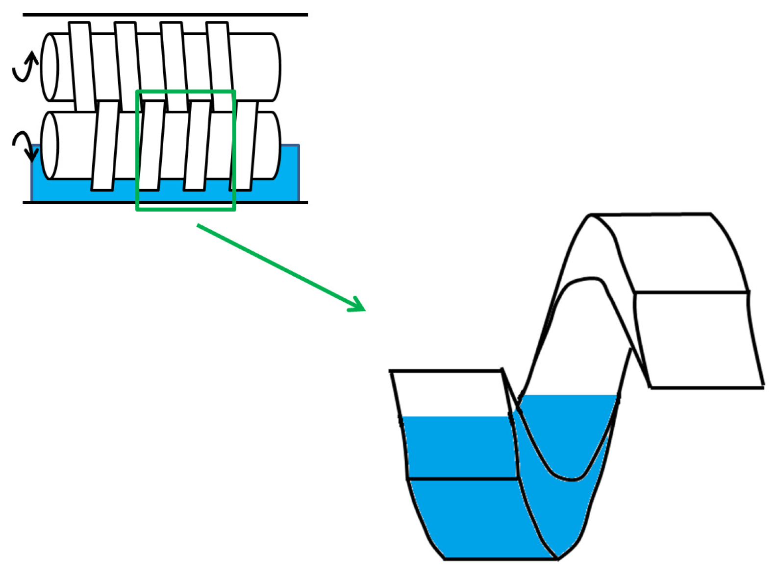
Figure 11.
(a) Five leakage locations in a twin screw extruder; (b) Flow network in a completely filled zone along one pitch length for a single-lobed screw (rectangular boxes represent C-shaped elements; square boxes represent inter-meshing elements).
Figure 11.
(a) Five leakage locations in a twin screw extruder; (b) Flow network in a completely filled zone along one pitch length for a single-lobed screw (rectangular boxes represent C-shaped elements; square boxes represent inter-meshing elements).

Figure 12.
Division of the twin screw in several perfectly-mixed reactors.
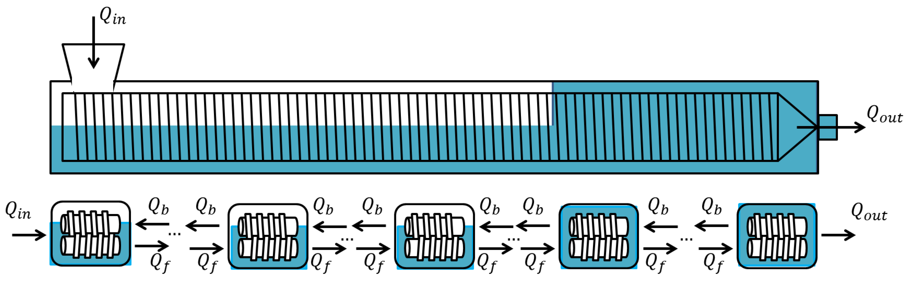
Figure 13.
CTR-in-series model validation. Solid line: model prediction; dashed line: experimental data.
Figure 13.
CTR-in-series model validation. Solid line: model prediction; dashed line: experimental data.

Figure 14.
Die pressure and outlet flow evolution following a step change in the screw rotation speed.
Figure 14.
Die pressure and outlet flow evolution following a step change in the screw rotation speed.

Figure 15.
Die pressure and outlet flow evolution following a step change in the feed flow.
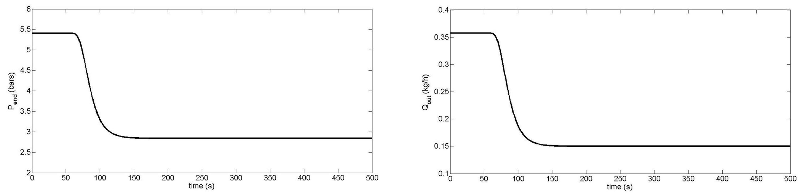
Figure 16.
Representation of the extruder zones.
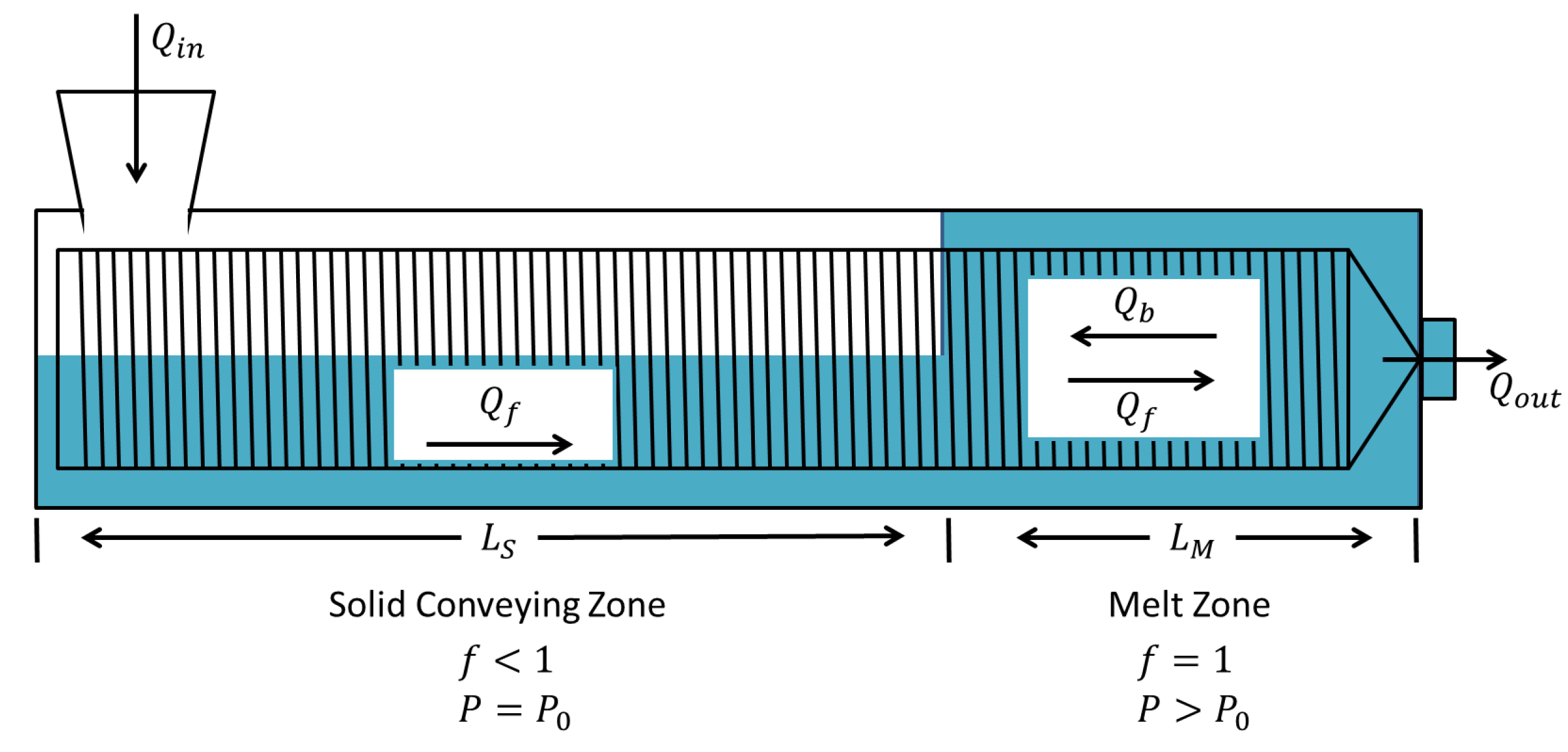
Figure 17.
Dynamic model numerical solution diagram.
Figure 18.
Change of spatial variable χ over the two extruder zones.

Figure 19.
Partial differential equation (PDE) model validation. Solid line: PDE model; dashed line: experimental data.
Figure 19.
Partial differential equation (PDE) model validation. Solid line: PDE model; dashed line: experimental data.
Figure 20.
Die pressure and outlet flow evolutions following a step change in the screw rotation speed.
Figure 20.
Die pressure and outlet flow evolutions following a step change in the screw rotation speed.
Figure 21.
Die pressure and outlet flow evolutions following a step change in the feed flow step.
Figure 22.
Scheme of the normal and the tangential contact forces.

Figure 23.
Multi-scale approach using discrete element modeling (DEM) and population balance modeling (PBM).
Figure 23.
Multi-scale approach using discrete element modeling (DEM) and population balance modeling (PBM).
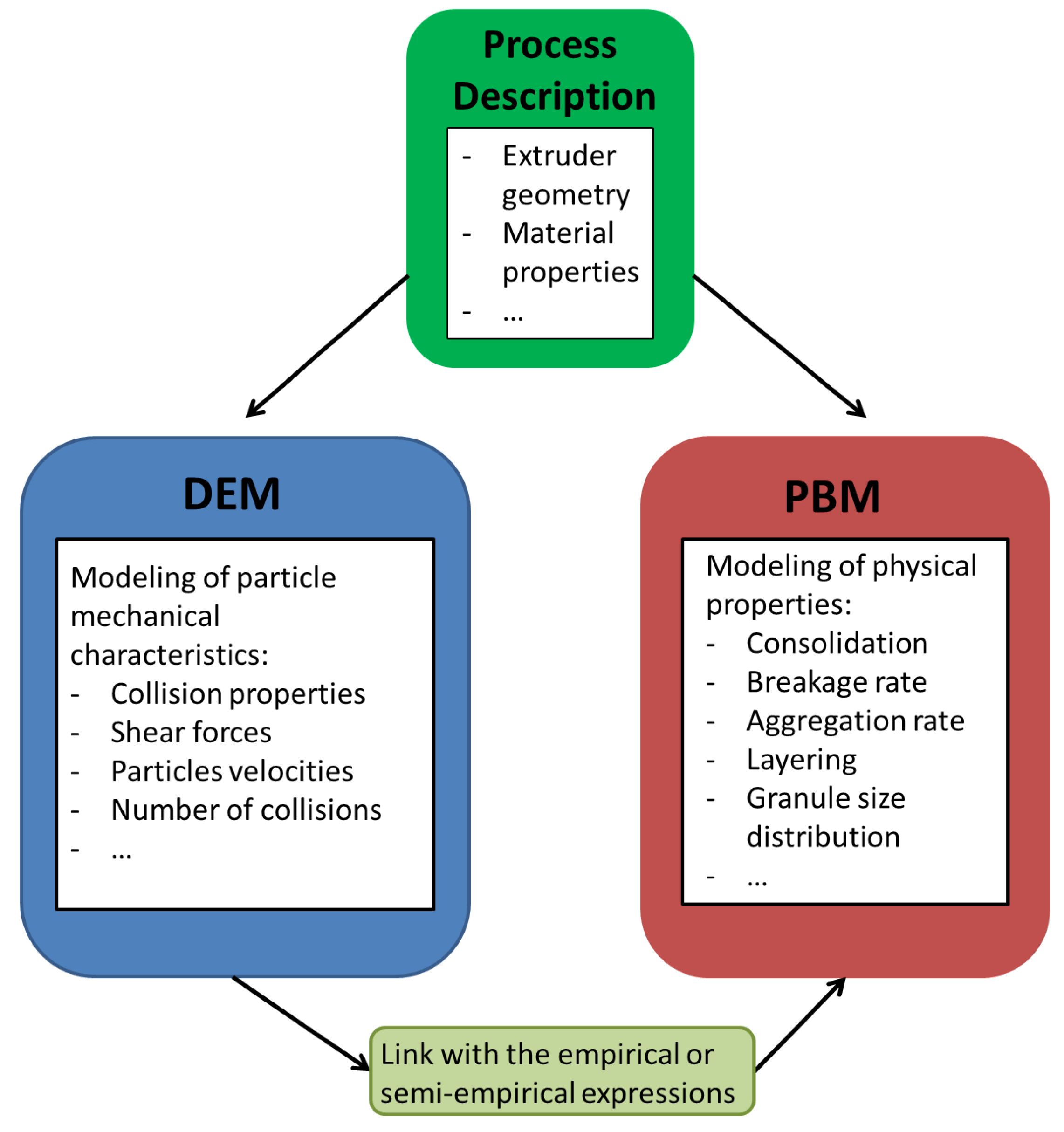
Figure 24.
Process black-box representation: input, output and disturbance.
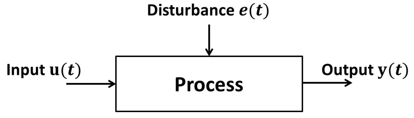
Figure 25.
Multilayer perceptron structure.

Figure 26.
Die pressure and outlet flow rate evolution following a step change in the screw rotation speed. Solid line: transfer function model; dashed line: experimental data.
Figure 26.
Die pressure and outlet flow rate evolution following a step change in the screw rotation speed. Solid line: transfer function model; dashed line: experimental data.

Figure 27.
Die pressure and outlet flow rate evolution following a step change in the input flow rate. Solid line: transfer function model; dashed line: experimental data.
Figure 27.
Die pressure and outlet flow rate evolution following a step change in the input flow rate. Solid line: transfer function model; dashed line: experimental data.

Figure 28.
Division of the extrusion system in different sections and moving boundaries of the filled zones.
Figure 28.
Division of the extrusion system in different sections and moving boundaries of the filled zones.

| Screw Geometry | Parameters | Values |
|---|---|---|
| Screw exterior diameter: | 18 mm | |
| Spacing screw: | 13 mm | |
| Screw pitch: ξ | 11 mm | |
| Screw threads number | 1 | |
| Total length: L | 150 mm | |
| Die geometry | Parameters | Values |
| Die diameter | 2.5 mm | |
| Die length | 6 mm | |
| Thermal properties | Parameters | Values |
| Specific heat capacity: | 5000 J/(kg K) | |
| Thermal conductivity: | 0.016 W/(m K) | |
| Material/barrel heat exchange coefficient: U | 1200 W/(m K) | |
| Barrel temperature: | 140 °C | |
| Material property | Parameter | Value |
| Density: ρ | 550 kg/m | |
| Yasuda-Carreau equations | Parameters | Values |
| b | 0.022 | |
| λ | 0.12 | |
| a | 10 | |
| 0.251 |
| Parameters | Values |
|---|---|
| n | 4 |
| 5.62 | |
| d | 0.063 |
Table 3.
Expressions of the forward and backward flow rates where and are screw geometric parameters, P is the pressure, f the filling ratio and V the reactor volume.
| Reactor i | ||
|---|---|---|
| Direct pitch | if or : | |
| Reverse pitch | if or : | |
| if or : | ||
| Die |
Table 4.
Estimated parameter values for the model of [35].
| Parameters | Values |
|---|---|
| n | 13 |
| 0.6 | |
| 0.16 |
| Parameters | Values | Absolute Confidence Intervals at 95 % |
|---|---|---|
| V | m | ± m |
| B | m | ± m |
| D | m/s | ± m/s |
© 2016 by the authors; licensee MDPI, Basel, Switzerland. This article is an open access article distributed under the terms and conditions of the Creative Commons Attribution (CC-BY) license (http://creativecommons.org/licenses/by/4.0/).
Share and Cite
MDPI and ACS Style
Grimard, J.; Dewasme, L.; Vande Wouwer, A. A Review of Dynamic Models of Hot-Melt Extrusion. Processes 2016, 4, 19. https://doi.org/10.3390/pr4020019
AMA Style
Grimard J, Dewasme L, Vande Wouwer A. A Review of Dynamic Models of Hot-Melt Extrusion. Processes. 2016; 4(2):19. https://doi.org/10.3390/pr4020019
Chicago/Turabian StyleGrimard, Jonathan, Laurent Dewasme, and Alain Vande Wouwer. 2016. "A Review of Dynamic Models of Hot-Melt Extrusion" Processes 4, no. 2: 19. https://doi.org/10.3390/pr4020019
Note that from the first issue of 2016, this journal uses article numbers instead of page numbers. See further details here.