Using Introspection to Collect Provenance in R

1
Computer Science Department, Mount Holyoke College, South Hadley, MA 01075, USA
2
Harvard Forest, Harvard University, Petersham, MA 01366, USA
3
Harvard College, Cambridge, MA 02138, USA
*
Author to whom correspondence should be addressed.
†
Current address: Google Inc., Mountain View, CA 94043, USA.
Informatics 2018, 5(1), 12; https://doi.org/10.3390/informatics5010012
Submission received: 1 December 2017
/
Revised: 25 February 2018
/
Accepted: 26 February 2018
/
Published: 1 March 2018
(This article belongs to the Special Issue Using Computational Provenance)
Abstract
:Data provenance is the history of an item of data from the point of its creation to its present state. It can support science by improving understanding of and confidence in data. RDataTracker is an R package that collects data provenance from R scripts (https://github.com/End-to-end-provenance/RDataTracker). In addition to details on inputs, outputs, and the computing environment collected by most provenance tools, RDataTracker also records a detailed execution trace and intermediate data values. It does this using R’s powerful introspection functions and by parsing R statements prior to sending them to the interpreter so it knows what provenance to collect. The provenance is stored in a specialized graph structure called a Data Derivation Graph, which makes it possible to determine exactly how an output value is computed or how an input value is used. In this paper, we provide details about the provenance RDataTracker collects and the mechanisms used to collect it. We also speculate about how this rich source of information could be used by other tools to help an R programmer gain a deeper understanding of the software used and to support reproducibility.
1. Introduction
Data and data analysis lie at the heart of science. Sharing scientific data is essential to allow scientists to build on each other’s work. However, such sharing will only occur if the data are trusted. Before using a dataset, a scientist would typically want to know the origin of the data, who was responsible, and how the raw data were manipulated to produce the published dataset. Data provenance describes this history of data and is useful to instil confidence in the data and to encourage its reuse [1].
To move from raw data to published data, there is a typical data analysis workflow involving cleaning the data to remove questionable values, extracting the subset of the data useful for the current analysis, performing the necessary statistical analysis, and publishing the results in the form of output data, plots, and/or papers describing the results.
There are several different types of provenance that help to describe this process. Static metadata capture details about data collection: where the data were collected, when, by whom, with what instruments, etc. Workflow provenance identifies the software used to process the data and how the data were passed from one tool to another as they were analyzed. Fine-grained execution provenance captures further detail internal to the software, recording precisely how each value was computed.
Besides improving the trustworthiness of data, provenance has the potential to help solve some important problems [2]. If a scientist discovers that a sensor has failed, for example, he or she might use provenance to determine what data were computed from that sensor so that they can be discarded. Conversely, if a scientist observes surprising results in output data, he or she might trace back to the inputs and discover in the process that a sensor has failed.
Provenance can also be used to help one scientist understand or reproduce another scientist’s work. For example, by examining provenance, a scientist could determine what bounds a second scientist had used to identify outliers in the data. If the first scientist felt those bounds were inappropriate, the analysis could be rerun with different bounds to see if that had an effect on the analysis results.
Fine-grained provenance can also support the debugging of scripts under development by capturing intermediate values. Using provenance, the scientist might trace backwards through the execution of the script to determine how a value was calculated and find the error without the need to set breakpoints or insert print statements and re-run the code, as is more commonly done. Fine-grained provenance also avoids the problems of nondeterminism caused by the use of random numbers in a simulation, or in concurrency, as the fine-grained provenance contains a precise history of the script execution that led to the error.
The focus of this paper is on a tool called RDataTracker and the value of the fine-grained provenance collected by RDataTracker for scripts written in R (https://www.r-project.org/), a language widely used by scientists for data analysis and visualization. In this paper we describe how we collect such provenance without directly modifying the R interpreter in order to make provenance capture available to scientists using the standard R interpreter. In previous papers [3,4], we introduced RDataTracker and DDG Explorer, a visualization tool that works with the provenance collected by RDataTracker. The version of RDataTracker described in these papers required the scientist to modify the script extensively to include commands identifying the provenance to collect. This paper describes a new implementation of RDataTracker that requires no annotation by the scientist and instead relies on introspection to identify the provenance to collect. In Section 2, we describe related work. In Section 3, we describe the provenance collected by RDataTracker. In Section 4, we describe the implementation of RDataTracker. In Section 5, we evaluate results. Our future plans are described in Section 6. Appendix A provides information about how to download and run RDataTracker.
2. Related Work
Capturing data provenance is a common feature of workflow tools, including Kepler [5], Taverna [6], and Vistrails [7], among others. The provenance captured by such tools describes the interaction among the tools used in a workflow and how the data flows between tools. While some scientists use workflow tools, they have not gained wide acceptance. In our experience, many scientists perform simpler data analyses that can be captured by a single script, such as an R or Python script, or by using tools such as R Markdown [8] or Jupyter notebooks (https://jupyter.org/).
Several systems allow the collection of workflow-like provenance without requiring the user to use workflow tools. Acuña et al. [9] describe a system that captures file-level provenance from ad hoc workflows written in Python. Burrito [10] collects provenance as a scientist works with multiple tools by inserting plug-ins that monitor shell commands, file activity and GUI activity. These are made available to the scientist with a variety of tools that allow the scientist to review and annotate past activity. ProvDB [11] and Ground [12] support storing provenance that is collected by external tools and then ingested into a database to support querying and analysis. YesWorkflow [13] constructs a workflow representation from a script based on stylized comments introduced by the scientists. McPhillips, et al. report that these can sometimes then be used to collect workflow-style provenance. These systems focus on gathering provenance at the level of workflow. In contast, our work focuses on fine-grained provenance collected at the statement level.
Thirty years ago Becker and Chambers [14] described a system for collecting provenance for top-level statements in the S language (a precursor of R). Though their approach is no longer viable (all objects in that version of S were stored in the file system), their paper foresees many of the applications and challenges of provenance today.
There are several other tools that collect provenance for R. recordr [15] is an R package that collects provenance concerning the libraries loaded and files read and written. It does this by overriding specific functions (such as read.csv) to record the provenance information prior to calling the predefined functions. The provenance recorded is thus at the level of files.
rctrack [16] is an R package that collects provenance with a focus on reproducibility. The provenance it collects consists of an archive containing input data files, scripts, output files, random numbers and session information, including details of the platform used as well as the version of R and loaded libraries. Having this level of detail is very valuable for reproducing results. The approach used in rctrack is to use R’s trace function to inject code into the functions that read and write files, generate random numbers, and make calls to external software (such as R’s system function). While including more information than recordr, this provenance is still primarily at the level of files and intended to support reproducibility. In contrast, the provenance collected by RDataTracker is finer grained and also serves the purpose of debugging.
Several other approaches to collecting fine-grained provenance involve modifying a language compiler or interpreter to perform the work. Michaelides et al. [17] modify the StatJR interpreter for the Blockly language to capture provenance used to provide reproducibility. Tariq et al. [18] modify the LLVM compiler framework to collect provenance at the entry and exit of functions. IncPy [19,20] uses a modified Python interpreter to cache function arguments and return values to avoid recomputation when the same function is called again with the same parameters. In CXXR [21], the read-eval-print loop inside the R interpreter is modified to collect provenance. The provenance collected is at the level of the global environment and is thus less detailed than the provenance collected by RDataTracker. Also, the provenance collected by CXXR is not made persistent and thus is only available for use within the current R session. These approaches require scientists to use non-standard implementations of language tools, which makes it harder to stay current as languages evolve and to get scientists to adopt these tools. In contrast, RDataTracker collects provenance both at the global level and within functions and saves the resulting provenance so that it can be loaded into other tools that support analysis, visualization and querying [4,22].
noWorkflow [23,24,25] is most similar to RDataTracker in implementation. noWorkflow collects fine-grained provenance from Python scripts using a combination of tracing function calls and program slicing. Like RDataTracker, noWorkflow works with the standard Python interpreter and relies on techniques that examine the runtime state of the script to collect provenance. The provenance collected by noWorkflow and RDataTracker are at a similar granularity, although the techniques used are different.
3. Provenance Collected by RDataTracker
The provenance collected by RDataTracker is stored in a specialized graph structure called a Data Derivation Graph (or DDG). In this section, we discuss the underlying provenance model and provide some simple examples.
3.1. Provenance Model
The provenance collected by RDataTracker includes both static information about the computing environment when an R script is run and dynamic information generated as the script executes. The former includes details about the computer hardware, operating system, R version, RDataTracker version, names and versions of loaded R libraries (if any), and names and timestamps of the R script and sourced scripts (if any). This information is collected in part using R’s sessionInfo command and is often essential for reproducing a particular result.
The dynamic information consists of the fine-grained provenance that is captured as the R script executes. It contains information about the statements that are executed, the variables used and assigned in these computations, the files and URLs that are read and written, and plots that are created. This fine-grained provenance is stored in a Data Derivation Graph (DDG). There are two primary types of nodes in a DDG: procedure nodes and data nodes, each with a set of subtypes. A procedure node corresponds to the execution of a statement, while a data node corresponds to a data value that is used or created by the statement. Procedure nodes are connected by control flow edges to capture the order in which the statements are executed. An output edge that goes from a procedure node to a data node identifies either a variable that is updated or a file that is written. An input edge that goes from a data node to a procedure node identifies a variable that is used or a file that is read.
Table 1 provides a complete list of the types of data nodes found in a DDG, while Table 2 provides a complete list of the types of procedural nodes found in a DDG.
The provenance information is written to the file ddg.json in PROV-JSON format (https://www.w3.org/Submission/2013/SUBM-prov-json-20130424/). Table 3 shows how the DDG nodes and edges are mapped into the PROV standard (https://www.w3.org/TR/2013/REC-prov-dm-20130430/). The direction of data edges in PROV is the reverse of their direction in DDGs. Thus, for example, the source of a wasGeneratedBy edge is the entity and the destination of the edge is the activity that produced it. When we store provenance in PROV format, we follow the PROV standard. When we display the edges in DDG Explorer, we use the direction defined in DDGs as we have found in our interactions with scientists that they find edges pointing in the direction of control flow to be more intuitive (the user can also change the direction of the arrows).
Each execution of an individual statement in the R script (or sourced script) is mapped to a unique procedure node in the DDG. RDataTracker records the node id, statement text (abbreviated), elapsed time when the statement completed execution, script number, and position of the statement in the script (start and end line and column). RDataTracker also creates start and finish nodes to mark the beginning and end of function calls, code blocks in control constructs (if, for, while, and repeat statements), sourced scripts, and the main script itself. Start and finish nodes provide an opportunity for DDG Explorer to present provenance at different levels of abstraction.
Each time a variable is assigned a value, a data node is created in the DDG with an output edge from the procedure node that assigned the value. Every use of that variable until the time that it is reassigned links to this data node with an input edge.
The JSON file contains simple data values (e.g., individual numbers and short strings). Because more complex data values (e.g., long strings, vectors, arrays, data frames, and lists) may be quite large, these are written as separate snapshot files with the name of the snapshot file stored in the JSON file. These files may be partial or complete copies of intermediate data values, depending on the current value of the max.snapshot.size parameter set by the scientist.
For each data node, RDataTracker records the node id, variable name, value, type, and scope information. Dimensions and individual column data types are also recorded for vectors, arrays, and data frames. Timestamps are recorded for intermediate values saved as snapshots. The original file location, timestamp, and MD5 hash value are recorded for input and output files and these files are copied to the provenance directory so they are saved even if the original files are later edited or deleted.
A visualizer such as DDG Explorer can use this information to display intermediate data values or the exact location of a statement in the original script (or sourced script) or to expand and contract sections marked by start and finish nodes.
3.2. DDG Examples
Figure 1 shows a simple R script along with the DDG that results from executing the script with function annotation turned off. Procedure nodes include start and finish nodes (green) that can be contracted to a single node to hide details, and operation nodes (yellow) that correspond to executed statements. Labels for the latter include an abbreviated form of the statement followed by the script number (0 = main script, 1 = first sourced script, etc) and line number in the source code. Procedure nodes are connected by control flow edges (blue arrows) that indicate the order of execution. Operation nodes may be connected by data flow edges (red arrows) to data nodes (blue) that indicate data objects created by or used by an operation. Here, the three operation nodes correspond to the three top-level statements in the R script.
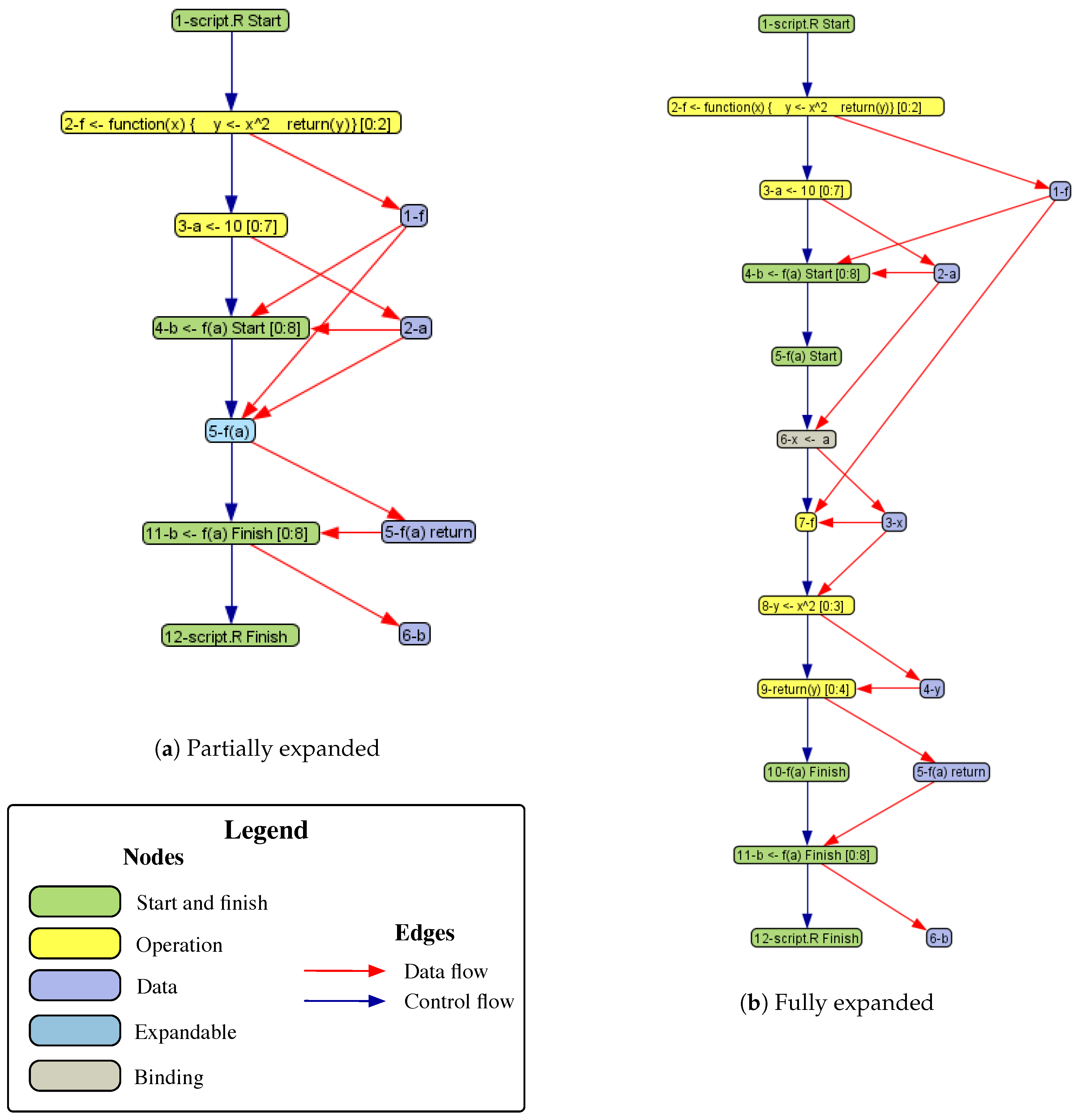
Figure 2a shows the DDG that results from running the same script with function annotation turned on. Here, the DDG is partially expanded to show start and finish nodes (green) that indicate the beginning and end of the evaluation of b <- f(a). An expandable node (light blue) indicates that the DDG contains further details for the evaluation of f(a).
Figure 2b shows the same DDG drawn with the function details fully expanded. This view of the DDG includes start and finish nodes (green) that indicate the beginning and end of the evaluation of b <- f(a) and f(a), a binding node (gray) that shows the assignment of the parameter a to the argument x, a procedure node for the internal statement y <- x⌃2, and a procedure node for creation of the function return value return(y). In DDG Explorer, the user can right-click on a data node to see its saved value or on a procedure node to see the script with the corresponding lines highlighted.
4. Implementation of RDataTracker
R is a very popular scripting language among scientists. Its strengths lie in its support for data analysis, particularly its statistics and plotting packages. R has a large user community with a strong history of developing and sharing open source packages, most notably via the CRAN repository (https://cran.r-project.org/). In this section, we first give an overview of some of R’s features, focusing on those of special interest for collecting provenance. We then discuss how we use R to collect provenance without modifying the R interpreter.
4.1. Background on R
A common strategy for analyzing data in R consists of reading data into one or more data frames (a two-dimensional tabular data structure), applying operations to extract the data to be used (e.g., the rows corresponding to a range of dates or the columns corresponding to the variables of interest), calling statistical functions to perform the desired analysis, and displaying the results in a series of plots. This process is often exploratory and the scientist will often refine a script repeatedly to develop a better understanding of the data under analysis.
While it is possible to write functions in R, many R scripts are written as a long sequence of commands, possibly with a few short functions. Furthermore, while a script is under development, it is not unusual for a scientist to execute the script one line or a few lines at a time, examining the results before continuing to write the script. Once a script is complete, it is also possible to execute it all at once. Many scripts are written to perform a particular analysis, often on a specific set of data. If the results are interesting, they may become the basis for an article or serve as a catalyst for further research. Other scripts are used repeatedly with different datasets, such as the scripts that create real-time graphs of meteorological and hydrological data at Harvard Forest (http://harvardforest.fas.harvard.edu/real-time-data-graphs).
R is optimized to perform vector operations. R also supports higher-order functions and provides a collection of built-in higher-order functions (e.g., to apply functions to data, filter data, and fold data), as is commonly seen in functional languages. Thus, while scientists tend not to write many functions, they call built-in and library functions frequently. Given the use of vector operations, applying functions to a vector is generally more efficient than looping over the vector to perform the same operation. As a result, R programmers often become very adept at functional programming.
For the purposes of collecting provenance, RDataTracker relies heavily on introspection capabilities available in R. For example, given a parsed statement, RDataTracker can find the variables that are used and set in the statement. From inside a function, RDataTracker can find out the expression that the caller used for each parameter passed. RDataTracker is also able to examine the call stack and the environments used to hold variable-value bindings at runtime. The use of these features by RDataTracker to capture detailed provenance is described in more detail in the remainder of this section.
4.2. Techniques Used to Collect Provenance
While modifying the R interpreter to collect provenance would simplify the job of finding the needed information, we decided instead to place the code that collects provenance in an R package (RDataTracker) that can be loaded into the standard R environment. In this way, we are able to share the package readily with R programmers without requiring them to use a specialized interpreter.
To collect provenance, RDataTracker combines work done statically prior to execution of the script with work done dynamically as the script executes (Figure 3). First the script is read from file and parsed. For each parsed statement, a DDGStatement object is created that includes the parsed statement as well as other information used to create the DDG. For example, the DDGStatement object includes a list of variables used or modified in the statement. By pre-calculating this information, RDataTracker saves time later when the statement is executed, particularly if the statement is inside a function or loop and possibly executed more than once. The DDGStatement object also contains an annotated version of the parsed statement that may contain additional function calls to aid in provenance collection. To execute the script, RDataTracker walks through the parsed DDGStatement objects, executing each in turn, and storing the relevant information in the DDG.
Section 4.2.1 discusses the static information stored in DDGStatement objects. Section 4.2.2 discusses the function calls we insert during parsing. Section 4.2.3 describes how we use R’s introspection mechanisms to construct the DDG. Section 4.2.4 discusses the granularity problem and how the user can limit the amount of provenance collected by RDataTracker.
4.2.1. Gathering Static Information About Statements
R scripts typically consist of statements written at the top level (that is, not inside any functions), function declarations, and calls to library functions. The script can be divided up into multiple R files that are combined using R’s source function, which essentially imports the source of one R file into another. R also provides several mechanisms to define classes, although these are more commonly used in defining reusable libraries than in the scripts developed by scientists to analyze their data. The provenance that we collect is done at the level of statements, whether those statements are top-level, within functions, within files included via a call to the source function, or within S4 classes.
To collect provenance, we analyze each line of source code to gather the static information that we will later refer to when collecting the execution provenance. This static information includes variables read and written, whether the statement reads from or writes to files, and whether the statement calls functions that are used to create plots. We store this information along with the parse tree for the statement in a data structure called a DDGStatement.
We examine the parse tree to identify which variables a statement uses or modifies. R has multiple assignment operators (<-, ->, =, <<-, and ->>) and an assign function. In addition, multiple values can be modified within an assignment. We divide the variables modified into two sets. If the statement being analyzed is an assignment statement, the variable assigned at the top level is stored as the variable set by the statement. If there are other assignments within the statement, we save those in a “possibly modified” set as, in general, we will not be able to determine if those variables are actually modified until the statement is executed (e.g., in the case of an if statement).
We similarly examine the parse tree for a statement to identify which variables it uses and record those in another set.
The second type of information we record concerns input to and output from the script. We record whether the statement calls any functions that read or write files or read URLs. This is done by comparing the names of functions called with a list of 22 functions that read files and 17 functions that write files. Later, when we execute the statement, we save copies of the files and also create nodes in the DDG to represent the file operations.
The third type of information records whether the function has any calls to functions that create or modify plots. A typical way to create a plot in R is to call a function such as jpeg or pdf, passing in the name of a file that the plot will be stored in when complete. This call opens a display device. Then a series of functions are called to add information to the plot, such as the data values, axis labels, and other information. These functions update the last display device that was opened, but they do so without explicitly passing the display device as a parameter. The display device is closed with a call to the dev.off function. Since the display device information is implicit and not a parameter to the functions that write to the display device, we treat the functions that update a plot as inputting a display device and outputting an updated display device. This additional information allows the user to query the DDG for information about how a plot was produced.
By gathering this information statically about what is read and written by each statement, whether it is variables, files, or plots, we then know at execution time what information we need to capture for each statement. This is particularly valuable for statements that may be executed frequently, such as those inside functions and loops.
4.2.2. Inserting Annotations
RDataTracker captures provenance for top-level statements at the point where they are executed with R’s eval function. However, we cannot use the same mechanism for statements inside functions or control constructs since these are executed in their entirety when eval is called. RDataTracker solves this problem by adding annotations that allow control to pass to RDataTracker during execution of the function or control construct. The annotations are added to the parse tree for the original function declaration or control construct and stored in the corresponding DDGStatement object. It is the annotated version of the original function or control construct that is actually executed.
For example, the following function declaration:
f <- function(x) {
     y <- x^2
     return(y)
}
is annotated as follows:
f <- function(x) {
    if (ddg.should.run.annotated("f")) {
        ddg.function()
        ddg.eval("y <- x^2")
        return(ddg.return.value(ddg.eval("y")))
    }
    else {
        y <- x^2
        return(y)
    }
}
If annotation is enabled for this function (ddg.should.run.annotated("f")), ddg.function captures function parameter and argument bindings, ddg.eval captures the provenance of statements internal to the function, and ddg.return.value creates the appropriate nodes and edges to connect the function return value to the site where the function is called. Otherwise no provenance is collected internal to the function.
In a similar way, if annotation inside loops is turned on, the scientist can decide on which iteration to begin collecting provenance and for how many iterations to continue collecting provenance. For each annotated iteration, a start node is created, a data node and edge are created for the index variable, statements internal to the loop are executed with ddg.eval, and a finish node is created. If one or more loops are not annotated, a Details Omitted node is created in the DDG to indicate this omission. If annotation inside loops is turned off, no provenance is collected internal to the loop.
4.2.3. Recording Provenance During Execution
As the script executes, we create procedural nodes, data nodes, and connecting edges, as described below.
Collecting the Provenance
To run a script, we walk through the list of DDGStatement objects, passing the annotated parsed R statement to R’s eval function to perform the actual execution. Upon eval’s return, we create an operation node that corresponds to the statement just executed and create an edge from the previously executed procedure node. We then look at the list of variables that are used in the statement and determine in which scope they are defined. To find the scope, we start with the environment associated with the current scope and search through its environment and its ancestor environments until we find the variable (this function is derived from the function available in Hadley Wickham’s pryr package and described in his book, Advanced R Programming [26], which we found to be extremely useful for understanding how R is implemented and how to gather provenance). We then look up the node in our data node table, using its name and scope to find the correct node. Once the correct node is found, we create a data flow edge from the data node to the new statement node. It is possible that a variable that is used does not have a data node because the variable is global and was set before the script executed. In that case, a data node is created and marked as originating from the pre-existing environment.
If the statement reads from a file or URL, we look at the call to the function that does the reading to identify the argument that corresponds to the file name or URL. Since R uses a combination of positional and named parameters, we first use R’s pmatch function to determine if the filename was passed with a named parameter. If there is no match based on a named parameter, we look for the parameter in the position where the filename should appear. We then evaluate the argument to find the name of the file. Once we have the filename, we verify that the file exists. If it does, we copy the file into the provenance directory, create a node for it, and create a data flow edge from the file node to the statement node.
Next, we find the variables that are set by the statement. For each of these, we create a data node, and record its name, value and scope in the data node table. We then create a data flow edge from the statement node to the data node.
Next, we identify the files written by the statement, using the same mechanism as for files being read. We save a copy of the file in the provenance directory, create a node for the file and an edge that goes from the statement node to the data node.
To keep track of graphic output, we find calls to the functions that open the graphics devices and record the filename that is provided with the call and remember that name until we see the dev.off function executed later. When the dev.off call is found, we determine which was the last graphics file opened, make a copy of that file and add a node and edge to the graph as for other files that are written.
We wrap the execution of eval with a handler so that we capture any warnings that occur when the statement executes. If the R interpreter produces an error or warning, we create an error node in the provenance whose value is the error message and link it to the node that corresponds to the statement that produced the error or warning. In R, errors generally result in a script ending prematurely and so it is easy for an R programmer to determine which R statement resulted in an error. However, it is often difficult to know which statement produced a warning message. By examining the provenance, the programmer can precisely identify the statement that produced the warning.
Collecting Provenance Internal to Functions
We save additional information on function calls and returns. When a function is called, we create nodes to record the binding of arguments in the call to parameters in the function definition. This binding is an implicit assignment and thus the nodes and edges created are similar to those for assignment statements. For example, Figure 2b shows a binding between argument a and parameter x in procedure node 6, when f(a) is executed.
R provides several ways to pass parameters to functions: positional, named, and dots. Using combinations of these features, the same R function can be called with a different number of parameters within a script. For example, consider the R function read.csv, which is used to read a CSV file into memory. Its signature is:
read.csv (file, header = TRUE, sep = ",", quote = "\"",
   dec = ".", fill = TRUE, comment.char = "", ...)
All of the following are legitimate calls to this function:
read.csv("mydata.csv")
read.csv("mydata.csv", FALSE)
read.csv(header = FALSE, file = "mydata.csv")
read.csv("mydata.csv", s=".", d=",", h=F)
read.csv("mydata.csv", s=".", d=",", h=F, nrows=100)
A parameter that is declared with a default value, such as “header = TRUE”, is an optional parameter. In the case of read.csv, the only required parameter is the file name since that does not have a default value. That is the form of the call in the first example. In the second example, there are 2 parameters passed by position: the filename and header. In the third example, the same two parameters are passed but this time by name. The fourth example shows that it is not necessary to use a parameter’s full name when passing by name; only a unique prefix is required. In this case, s is sep, d is dec and h is header. The value FALSE can also be passed as F. Finally, the last example passes a parameter by name where the parameter is not named in the call to read.csv. In this case, the parameter matches ... and will be passed on to a method called by read.csv, in this case the more general read.table function. The variety of parameter passing mechanisms makes it challenging to determine which arguments are bound to which parameters so that the correct edges are created in the provenance graph.
To determine which arguments are bound to which parameters, we use R’s match.call function. First, we use the call stack to find the function that is being called as well as the expression that calls the function. We pass these to match.call, which returns a call in which all of the arguments used in the function call are specified by their full names, essentially turning everything into named parameters. We then walk the parameter list in the expanded call to determine the binding nodes and their input and output data nodes.
Return Values
On return from a function, we create a data node to hold the return value. This will then be linked into the DDG based on how the return value is used.
To properly connect values returned by functions to the site where those values are used, RDataTracker creates a table that contains information about function return values. For each value returned, RDataTracker records: the text of the function call, such as f(a); the line number where the function was called; whether the return value has already been connected to its call site; and the unique id of the data node holding the return value.
RDataTracker adds an entry to this table when the script executes a return statement and uses this table when it completes the provenance for a statement that calls a function. It looks for an entry in the table for a function that matches the text from the call’s line number and has not yet been used. By using all three pieces of information, we can be sure that we are getting the correct return value even for recursive functions, or multiple calls to the same function with the same or different parameters from within a single statement.
4.2.4. Granularity
It comes as no surprise that collecting fine-grained provenance has associated costs in terms of script execution time, file storage, and the size and complexity of the resulting provenance. Depending on the script, the use of higher-order functions and/or iterative loops may greatly increase the number of nodes and edges (and associated metadata) in the DDG. Saving full snapshots of large data objects that are updated frequently (as is often the case for data frames) can use a lot of storage space. Both scenarios are common in the scripts that scientists use.
RDataTracker addresses this problem by allowing the user to limit the amount of provenance that is collected for a particular script execution. In particular, there are three ways to limit the detail:
- Limit the size of intermediate values that are saved.
- Control whether nodes are created during the execution of a function or whether a function call is represented with a single procedural node. This can be done globally, so that all functions are treated the same, or this feature can be enabled or disabled for individual functions.
- Control whether fine-grained provenance is collected internal to control constructs, and if it is, limit the number of iterations of a loop for which provenance is collected.
The granularity of provenance required for particular applications remains an interesting research question. Use of one or more of the features above can improve the performance of RDataTracker significantly, but at the risk of failing to capture critical information. In the long run, we expect that the choice of application will guide the choice of granularity. Some applications, such as script debugging, will no doubt profit from collecting as much detail as possible. Other applications, such as identifying script inputs and outputs, may require much less detail. For scripts that are non-deterministic, it may be better to err on the side of collecting more detail, because rerunning the script to collect more detailed provenance may lead to a different result.
5. Evaluation
When RDataTracker collects detailed provenance we expect a significant slowdown in execution since each line of the original script results in provenance being saved. Each line results in the creation of a procedural node, most lines produce at least one output data node and use at least one input data node, and the edges associated with these nodes must be created. Furthermore, saving copies of input and output data files and plots, as well as intermediate data (which can include large dataframes) is time consuming.
In this section, we present the results of timing script execution with and without RDataTracker collecting provenance. Our goal is to measure two things: the slowdown caused by saving more detail in the DDG, and the slowdown caused by creating snapshots of intermediate values.
To measure these effects we used slightly modified versions of scripts used at Harvard Forest. One script, the Met script, processes data from the Fisher Meteorological Station. The second script, the Hydro script, processes data from six Hydrological Stations in the Prospect Hill Tract. Both of these scripts create tables and graphs for the Harvard Forest web page (http://harvardforest.fas.harvard.edu/real-time-data-graphs). For both scripts, the timing tests were run on saved input files, rather than real-time data, and the output was saved to a collection of files, rather than moved to the website. This avoided any timing variations that might be due to network speed or different input data values.
Table 4 provides further detail on the scripts. In the table, a top-level statement is a statement that is not inside a function. Note that a control construct at the top level counts as a single statement. The number of top-level statements will match the number of operational nodes created in an execution captured at detail level 0, as described below.
Both scripts were run with various combinations of detail level and snapshot size. The levels of detail were as follows:
- No DDG: The original script with no provenance collected.
- Detail level 0: Collect provenance only for top-level statements.
- Detail level 1: Collect provenance internal to functions and internal to loops but only for a single loop iteration.
- Detail level 2: Collect provenance internal to functions and internal to loops for up to 10 iterations of each loop.
- Detail level 3: Collect provenance internal to functions and internal to loops for all loop iterations.
The snapshot sizes were as follows:
- No DDG: The original script with no provenance collected.
- No snapshots: Collect provenance but save no snapshots.
- 10K snapshots: Save snapshots up to 10K bytes per snapshot.
- 100K snapshots: Save snapshots up to 100K bytes per snapshot.
- Max snapshots: Save snapshots of any size.
The tests were performed on a MacBook Pro with 4 cores, using 2.3 GHz Intel Core i7 processor and 16 GB of RAM. Each test was repeated five times and the average value was used to produce the graphs.
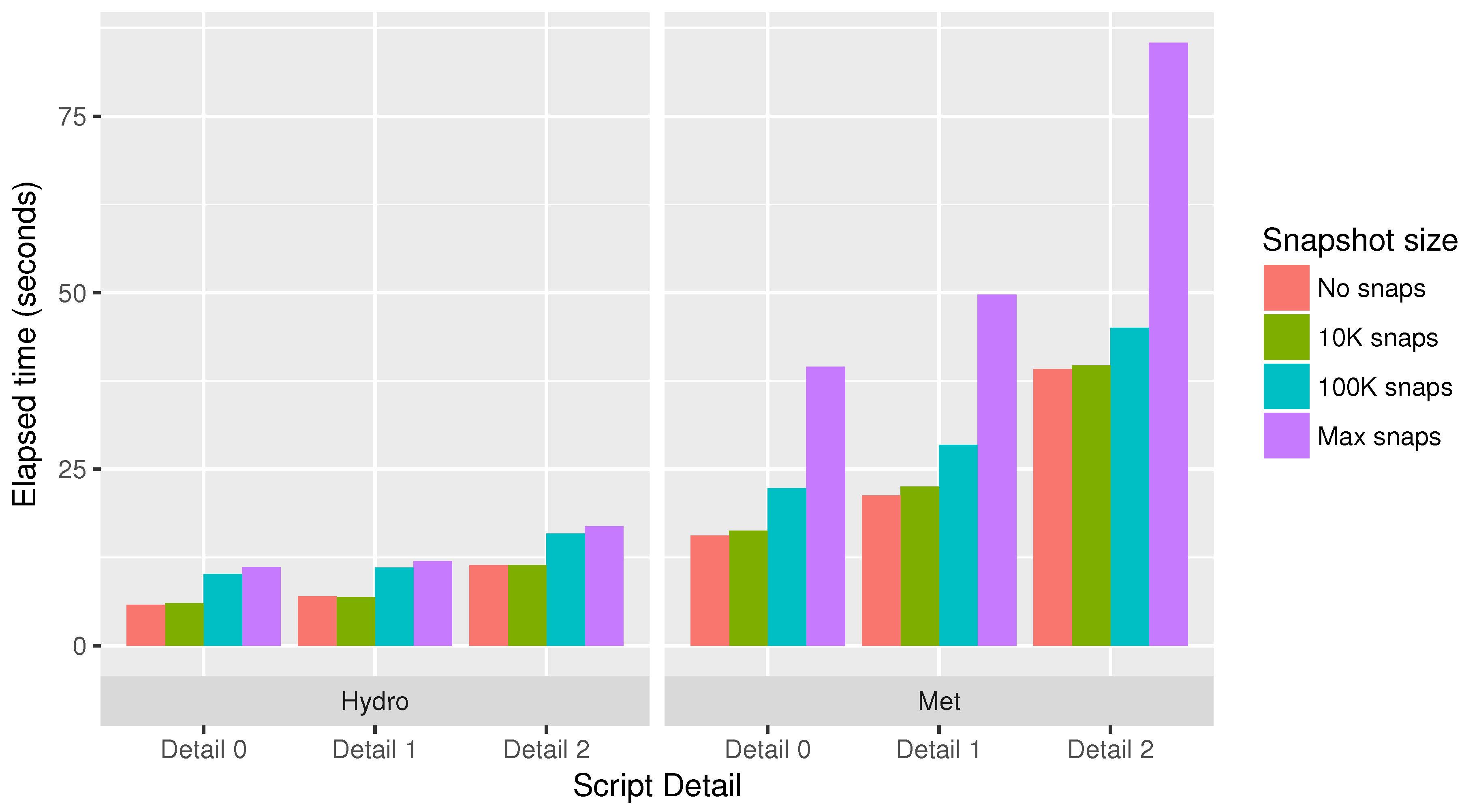
Figure 4 shows the results of running the timing analysis as the level of detail and size of snapshots saved was varied. As expected, the performance slowed down as the level of detail captured in the provenance increased. At detail level 3 with no snapshots (not shown), the elapsed time for the Met script was 678 seconds while the Hydro script did not complete after several hours, representing an unacceptable slowdown. The long computation times and large DDG sizes for level 3 (see Table 5 below) were caused by loops with large numbers of iterations (both scripts) and embedded calls to user-defined functions (Hydro script).
Figure 4 also shows that the performance slowed down as the size of the snapshots increased. It is interesting to note that, at least for these scripts, there is little difference in execution time between saving no snapshots and saving snapshots that are each limited to 10K in size. Even small, incomplete snapshots might be helpful for finding certain problems with code that manipulates data frames. For example, a programmer could verify that the equation used to compute the value for a new column in the data frame is generally correct, by examining just a few rows of the data frame.
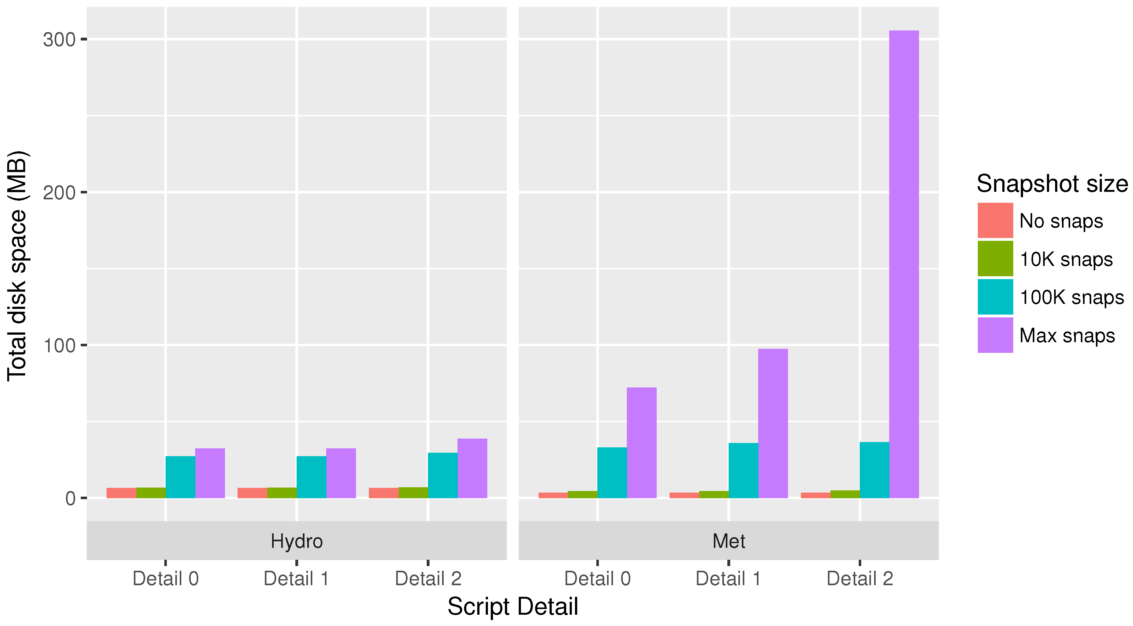
Figure 5 shows the amount of disk space used to store the provenance data recorded at different detail levels and snapshot sizes. As expected, if a large data frame is repeatedly modified, and RDataTracker is saving large snapshots, the amount of disk space used to store the snapshots can grow considerably. As with the runtime, we see little change in the total disk space used when going from no snapshots to snapshots limited to 10K.
Table 5 shows the numbers of nodes and edges in the provenance graph for various levels of detail. As expected, these numbers increased significantly as the level of detail increased. In particular, as these two scripts use for loops in several places to iterate over the rows of a data frame, we see a large jump as we go from detail level 1 (saving 1 loop iteration), to detail level 2 (saving 10 loop iterations), to detail level 3 (saving all loop iterations). It seems reasonable, then, that size of detail level 2 is somewhat less than 10 times the size of detail level 1, while the size of detail level 3 for the Met script shows a much larger jump since one of its loops is iterated 2880 times.
In general, performance slows down proportionally to the amount of data collected. We would also expect different performance characteristics depending upon the nature of the script. Slowdown can be caused by loops, when we are collecting provenance internal to loops; functions, when significant amounts of the computation are done inside user-defined functions and we are collecting provenance internal to functions; and intermediate data, when the calculations are working with large data frames or other data structures and making frequent updates to them.
It is not possible to draw broad conclusions about the performance of RDataTracker from the results of running RDataTracker on just these two scripts. Scripts written by other developers and in other domains may have a programming style that results in either better or worse performance. While our expectation is that the ways in which top-level statements, functional programming, and loops are used will have an impact on RDataTracker’s performance, we have not yet gathered the scripts needed to do this larger evaluation and draw meaningful conclusions.
In addition, new R packages are constantly being developed, some of which may have a significant impact on how scientists write R code and what types of provenance should be collected. For example, the pipe operator provided in the magrittr (https://github.com/tidyverse/magrittr) package allows for the output of one expression to be piped directly into another expression without the need to introduce intervening variables [27]. It may be desirable to collect provenance for each expression involved in a pipe, rather than just at the completion of the entire statement.
6. Future Work
We plan to introduce other features that give the programmer more control over how much detail is collected at different parts of the script execution. For example, the ability to turn provenance collection on and off dynamically during script execution would allow the scientist to decide when to pay the cost associated with fine-grained provenance collection. In particular, we expect fine-grained provenance to be most beneficial during development and debugging of a script, and we are working on tools that will make the provenance more accessible via a specialized provenance-aware debugger. Features that a provenance-aware debugger could provide include a history of the values that a variable assumes over time, or a list of places where the type of the value assigned to a variable has changed (a common problem in languages with dynamic typing).
Efficiency could also be gained by reducing the number and size of snapshots. For example, rather than storing an entire data frame after it is updated, we could save a data frame only when a large portion of it changes. For smaller changes, if they are deterministic operations, we could simply re-execute the instructions saved in the DDG to calculate an updated value for the data frame on demand.
In general, the primary direction of our future work will be to build tools that can leverage detailed provenance to perform tasks that are useful to scientists, without the need to view or interact with the provenance directly. Our experience with users to date suggests that few if any scientists will want to examine lengthy DDGs to understand the behavior of their own scripts or scripts written by others, but they may adopt tools that prove useful in their work. Thomas Pasquier and Matthew Lau, for example, have developed a tool that uses the provenance collected by RDataTracker to create a cleaned version of an R script that can be packaged and shared with other scientists [28]. Tools that use provenance to identify and save the items essential for reproducing a result (user input, data read from local files or urls, random numbers, etc.) have the potential to improve data repositories such as Dataverse (https://dataverse.org/) and DataONE (https://www.dataone.org/).
7. Conclusions
RDataTracker provides a fine-granularity view of provenance. It does this by building upon the introspection capabilities of R and by parsing each statement prior to passing it to the interpreter in order to determine what data to collect. While provenance collection could be done more efficiently from within the interpreter, the presence of strong introspection capabilities opens a lot of possibilities for developing tools that have a deep understanding of program behavior while still using the standard interpreter.
RDataTracker has the ability to produce a complete execution trace of each statement executed and to save all intermediate data values. As our evaluation shows, this level of granularity has associated costs and may be more than what is needed for many applications. Our next steps will be to provide more ways to dynamically control the level of detail collected, and to build tools that leverage provenance to provide value for R programmers, including advanced debugging features and support for reproducibility.
Acknowledgments
This work was funded by grants from the National Science Foundation (DEB-1237491, DBI-1459519, and SSI-1450277) and by Harvard Forest and a Harvard University Bullard Fellowship and is a contribution from the Harvard Forest Long-Term Ecological Research (LTER) program. We also would like to thank the following people who contributed to the implementation of RDataTracker: Elizabeth Fong, Connor Gregorich-Trevor, Alex Liu, Yada Pruksachatkun, and Moe Pwint Phyu. We also wish to acknowledge our research collaborators who have contributed ideas that have helped form RDataTracker: Aaron Ellison, Matthew Lau, Lee Osterweil, Thomas Pasquier, and Margo Seltzer.
Author Contributions
Barbara Lerner and Emery Boose were the principal designers and authors of RDataTracker and authors of the article. Luis Perez made substantial improvements to the design and implementation of RDdataTracker as an REU student at Harvard Forest.
Conflicts of Interest
The authors declare no conflict of interest. The funding sponsors had no role in the design of the study; in the collection, analyses, or interpretation of data; in the writing of the manuscript; or in the decision to publish the results.
Appendix A. Using RDataTracker
RDataTracker is freely available on GitHub as an R package (https://github.com/End-to-end-provenance/RDataTracker). To install it, use the install_github function in the R devtools library. To capture data provenance for an R script, set the working directory, load the RDataTracker package with the R library function, and enter the following command:
> ddg.run("script.R")
where “script.R” is an R script in the working directory. The ddg.run function will execute the script and save the provenance information (in the form of a Data Derivation Graph or DDG) to the file system. To view the DDG, enter the following command:
> ddg.display()
This command will call up the visualization tool (DDG Explorer), display the last DDG created, and allow the user to query the DDG in various ways.
The ddg.run function has several optional parameters that control how it works, including whether to collect provenance inside functions and control constructs, the number of the first loop iteration to annotate, the maximum number of loop iterations to annotate, and the maximum size for objects saved in snapshot files. It is also possible to execute the script one line at a time with an option to view the DDG after each line is executed.
References
- Pasquier, T.; Lau, M.K.; Trisovic, A.; Boose, E.R.; Couturier, B.; Crosas, M.; Ellison, A.M.; Gibson, V.; Jones, C.R.; Seltzer, M. If these data could talk. Sci. Data 2017, 4, 170114. [Google Scholar] [CrossRef] [PubMed]
- Miles, S.; Groth, P.; Branco, M.; Moreau, L. The requirements of recording and using provenance in e-Science experiments. J. Grid Comput. 2005, 5, 1–25. [Google Scholar] [CrossRef] [Green Version]
- Lerner, B.S.; Boose, E.R. RDataTracker: Collecting provenance in an interactive scripting environment. In Proceedings of the 6th USENIX Workshop on the Theory and Practice of Provenance, Cologne, Germany, 12–13 June 2014; USENIX Association: Cologne, Germany, 2014. [Google Scholar]
- Lerner, B.S.; Boose, E.R. RDataTracker and DDG Explorer—Capture, visualization and querying of provenance from R scripts. In Proceedings of the 5th International Provenance and Annotation Workshop, Cologne, Germany, 9–13 June 2014; IPAW: Cologne, Germany, 2014. [Google Scholar]
- Altintas, I.; Barney, O.; Jaeger-Frank, E. Provenance Collection Support in the Kepler Scientific Workflow System. In Proceedings of the 1st International Provenance and Annotation Workshop, Chicago, IL, USA, 3–5 May 2006; Springer: Berlin/Heidelberg, Germany, 2006; pp. 118–132. [Google Scholar]
- Zhao, J.; Goble, C.; Stevens, R.; Turi, D. Mining Taverna’s semantic web of provenance. Concurr. Comput. Pract. Exp. 2008, 20, 463–472. [Google Scholar] [CrossRef]
- Silva, C.T.; Anderson, E.; Santos, E.; Freire, J. Using VisTrails and Provenance for Teaching Scientific Visualization. Comput. Graph. Forum 2011, 30, 75–84. [Google Scholar] [CrossRef]
- Baumer, B.; Cetinkaya-Rundel, M.; Bray, A.; Loi, L.; Horton, N.J. R Markdown: Integrating a Reproducible Analysis Tool into Introductory Statistics. Technol. Innov. Stat. Educ. 2014, 8. Available online: https://escholarship.org/uc/item/90b2f5xh (accessed on 28 February 2018). [CrossRef]
- Acuña, R.; Lacroix, Z.; Bazzi, R.A. Instrumentation and Trace Analysis for Ad-hoc Python Workflows in Cloud Environments. In Proceedings of the 2015 IEEE 8th International Conference on Cloud Computing, New York, NY, USA, 27 June–2 July 2015; pp. 114–121. [Google Scholar]
- Guo, P.J.; Seltzer, M. BURRITO: Wrapping Your Lab Notebook in Computational Infrastructure. In Proceedings of the 4th USENIX Workshop on the Theory and Practice of Provenance, Boston, MA, USA, 14–15 June 2012; USENIX Association: Boston, MA, USA, 2012. [Google Scholar]
- Miao, H.; Chavan, A.; Deshpande, A. ProvDB: Lifecycle Management of Collaborative Analysis Workflows. In Proceedings of the 2nd Workshop on Human-In-the-Loop Data Analytics, Chicago, IL, USA, 14 May 2017; ACM: New York, NY, USA, 2017; pp. 7:1–7:6. [Google Scholar]
- Hellerstein, J.M.; Sreekanti, V.; Gonzalez, J.E.; Dalton, J.; Dey, A.; Nag, S.; Ramachandran, K.; Arora, S.; Bhattacharyya, A.; Das, S.; et al. Ground: A Data Context Service. In Proceedings of the Conference on Innovative Data Systems Research ’17, Chaminade, CA, USA, 8–11 January 2017; CIDR: Chaminade, CA, USA, 2017. [Google Scholar]
- McPhillips, T.; Aulenbach, S.; Song, T.; Belhajjame, K.; Kolisnik, T.; Bocinsky, K.; Dey, S.; Jones, C.; Cao, Y.; Freire, J.; et al. YesWorkflow: A User-Oriented, Language-Independent Tool for Recovering Workflow Information from Scripts. Int. J. Digit. Curation 2015, 10, 298–313. [Google Scholar] [CrossRef]
- Becker, R.; Chambers, J. Auditing of data analyses. SIAM J. Sci. Stat. Comput. 1988, 9, 747–760. [Google Scholar] [CrossRef]
- Slaughter, P.; Jones, M.B.; Jones, C.; Palmer, L. Recordr. Available online: https://github.com/NCEAS/recordr (accessed on 27 February 2018).
- Liu, Z.; Pounds, S. An R package that automatically collects and archives details for reproducible computing. BMC Bioinform. 2014, 15, 138. [Google Scholar] [CrossRef] [PubMed]
- Michaelides, D.T.; Parker, R.; Charlton, C.; Browne, W.J.; Moreau, L. Intermediate Notation for Provenance and Workflow Reproducibility. In International Provenance and Annotation Workshop; number 9672 in Lecture Notes in Computer Science; Mattoso, M., Glavic, B., Eds.; Springer International Publishing: Cham, Switzerland, 2016; pp. 83–94. [Google Scholar]
- Tariq, D.; Ali, M.; Gehani, A. Towards Automated Collection of Application-level Data Provenance. In Proceedings of the 4th USENIX Conference on Theory and Practice of Provenance, Boston, MA, USA, 14–15 June 2012; USENIX Association: Berkeley, CA, USA, 2012. [Google Scholar]
- Guo, P.J.; Engler, D. Towards Practical Incremental Recomputation for Scientists: An Implementation for the Python Language. In Proceedings of the 2nd USENIX Workshop on the Theory and Practice of Provenance, San Jose, CA, USA, 22 February 2010; USENIX Association: Berkeley, CA, USA, 2010. [Google Scholar]
- Guo, P.J.; Engler, D. Using Automatic Persistent Memoization to Facilitate Data Analysis Scripting. In Proceedings of the 2011 International Symposium on Software Testing and Analysis, Toronto, ON, Canada, 17–21 July 2011; ACM: New York, NY, USA, 2011; pp. 287–297. [Google Scholar]
- Silles, C.A.; Runnalls, A.R. Provenance-Awareness in R. In Proceedings of the 3rd International Provenance and Annotation Workshop, Troy, NY, USA, 15–16 June 2010; IPAW: Troy, NY, 2010; pp. 64–72. [Google Scholar]
- Pasquier, T. CamFlow/cytoscape.js-prov: Initial release. Zenodo 2017. [Google Scholar] [CrossRef]
- Murta, L.; Braganholo, V.; Chirigati, F.; Koop, D.; Freire, J. NoWorkflow: Capturing and Analyzing Provenance of Scripts. In Proceedings of the 5th International Provenance and Annotation Workshop, Cologne, Germany, 9–13 June 2014; IPAW: Cologne, Germany, 2014. [Google Scholar]
- Pimentel, J.F.N.; Braganholo, V.; Murta, L.; Freire, J. Collecting and Analyzing Provenance on Interactive Notebooks: When IPython meets noWorkflow. In Proceedings of the 7th USENIX Workshop on the Theory and Practice of Provenance, Edinburgh, Scotland, 8–9 July 2015; USENIX Association: Edinburgh, Scotland, 2015. [Google Scholar]
- Pimentel, J.F.; Freire, J.; Murta, L.; Braganholo, V. Fine-Grained Provenance Collection over Scripts Through Program Slicing. In Proceedings of the 6th International Provenance and Annotation Workshop, McLean, VA, USA, 7–8 June 2016; Mattoso, M., Glavic, B., Eds.; Lecture Notes in Computer Science; Springer: Cham, Switzerland, 2016; Volume 9672. [Google Scholar]
- Wickham, H. Advanced R; The R Series; Chapman and Hall/CRC: Boca Raton, FL, USA, 2014. [Google Scholar]
- Grolemund, G.; Wickham, H. R for Data Science; Chapter 18: Pipes; O’Reilly: Sebastopol, CA, USA, 2017. [Google Scholar]
- Pasquier, T.; Lau, M.K.; Han, X.; Fong, E.; Lerner, B.S.; Boose, E.; Crosas, M.; Ellison, A.; Seltzer, M. Sharing and Preserving Computational Analyses for Posterity with encapsulator. IEEE Comput. Sci. Eng. 2018. under review. [Google Scholar]
Figure 1.
DDG without function annotation.
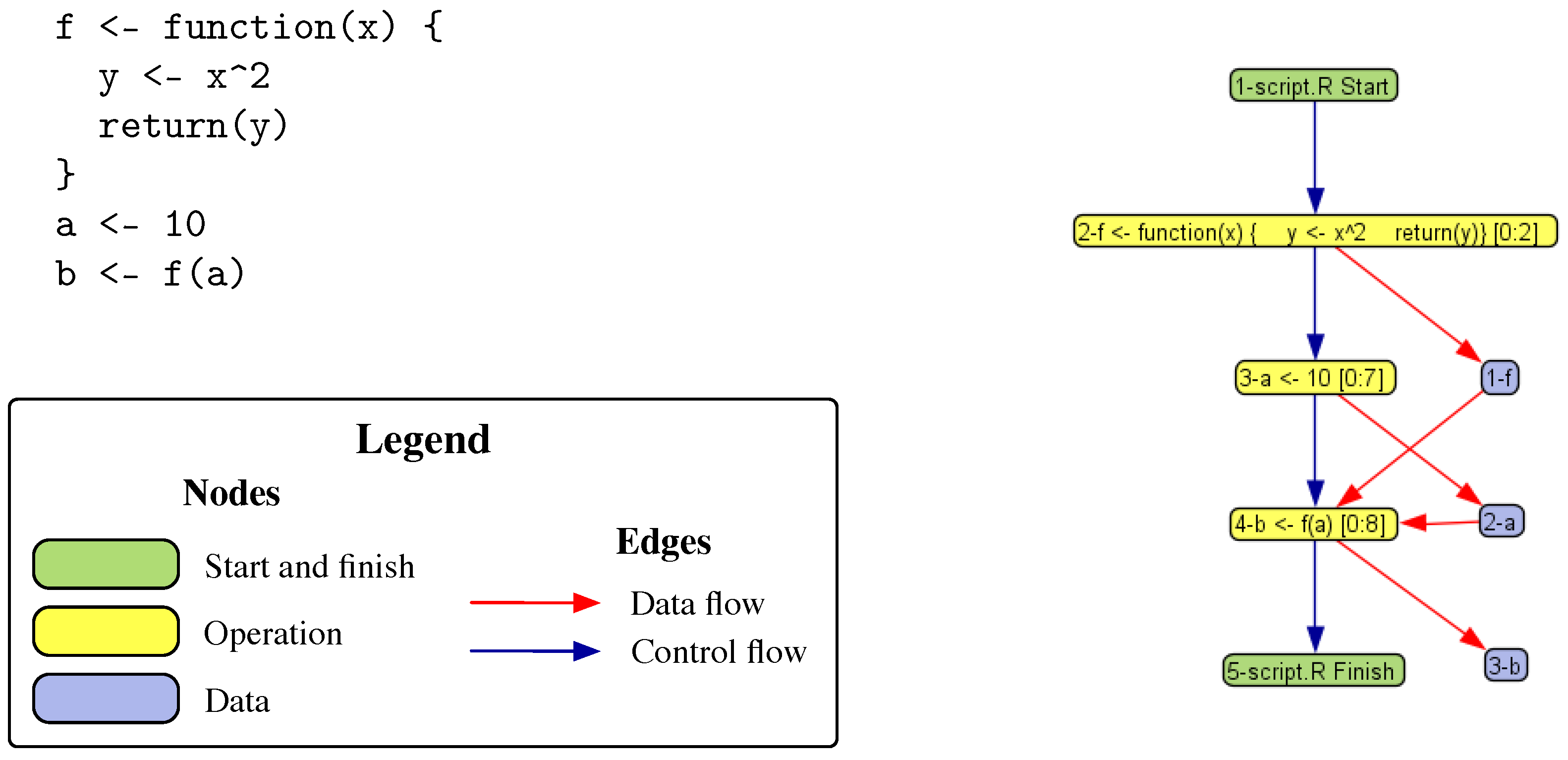
Figure 2.
DDG with function annotation.

Figure 3.
Architecture of RDataTracker.

Figure 4.
Runtime with different snapshot sizes and detail levels.

Figure 5.
Disk space used with different snapshot sizes and detail levels.


Table 1.
Data node types.
| Node Type | Primary Attribute | Use |
|---|---|---|
| Data | Value | Scalar values and short strings |
| File | Location of a saved copy of the file | Files that are read or written |
| Snapshot | Location of the snapshot file | Complex data structures and long strings |
| URL | URL | URLs that are read from |
| Exception | Error message | Warnings or errors generated during execution |
Table 2.
Procedural node types.
| Node Type | Primary Attribute | Use |
|---|---|---|
| Operation | Location of the statement | Execute a statement |
| Binding | Parameter being bound and argument | Capture parameter passing |
| Start | None | Precedes execution of a control construct or function |
| Finish | None | Follows execution of a control construct or function |
| Incomplete | None | Indicates that detailed provenance is not collected on all executions of a loop |
Table 3.
DDG and PROV representations.
| DDG Representation | PROV Representation |
|---|---|
| Procedure node | activity |
| Data node | entity |
| Control flow edge | wasInformedBy |
| Input edge | used |
| Output edge | wasGeneratedBy |
Table 4.
Script characteristics.
| Script | Input Files | Data Values | Output Files | Top-Level Statements | Functions | Loops |
|---|---|---|---|---|---|---|
| Met | 2 | 27,320 | 6 | 149 | 0 | 7 |
| Hydro | 6 | 82,294 | 3 | 141 | 3 | 8 |
Table 5.
Size of provenance graph.
| Hydro | Hydro | Hydro | Met | Met | Met | Met | |
|---|---|---|---|---|---|---|---|
| Detail 0 | Detail 1 | Detail 2 | Detail 0 | Detail 1 | Detail 2 | Detail 3 | |
| Procedure Nodes | 141 | 296 | 1282 | 149 | 199 | 564 | 18270 |
| Data Nodes | 162 | 224 | 738 | 168 | 186 | 367 | 6306 |
| Edges | 493 | 913 | 4045 | 557 | 663 | 1653 | 25928 |
© 2018 by the authors. Licensee MDPI, Basel, Switzerland. This article is an open access article distributed under the terms and conditions of the Creative Commons Attribution (CC BY) license (http://creativecommons.org/licenses/by/4.0/).
Share and Cite
MDPI and ACS Style
Lerner, B.; Boose, E.; Perez, L. Using Introspection to Collect Provenance in R. Informatics 2018, 5, 12. https://doi.org/10.3390/informatics5010012
AMA Style
Lerner B, Boose E, Perez L. Using Introspection to Collect Provenance in R. Informatics. 2018; 5(1):12. https://doi.org/10.3390/informatics5010012
Chicago/Turabian StyleLerner, Barbara, Emery Boose, and Luis Perez. 2018. "Using Introspection to Collect Provenance in R" Informatics 5, no. 1: 12. https://doi.org/10.3390/informatics5010012
Note that from the first issue of 2016, this journal uses article numbers instead of page numbers. See further details here.