
Coherent Mortality Forecasting for Less Developed Countries †


1
Department of Economics and Finance, University of Guelph, Guelph, ON N1G 2W1, Canada
2
Department of Mathematics and Statistics, Concordia University, Montreal, QC H3G 1M8, Canada
3
Department of Econometrics and OR, Tilburg University, 2591 TV The Hague, The Netherlands
*
Authors to whom correspondence should be addressed.
†
An earlier version of this paper was circulated under the title “Modeling and Forecasting Chinese Population Dynamics in a Multi-population Context”.
Risks 2021, 9(9), 151; https://doi.org/10.3390/risks9090151
Submission received: 30 June 2021
/
Revised: 14 August 2021
/
Accepted: 18 August 2021
/
Published: 24 August 2021
(This article belongs to the Special Issue Longevity Risk Modelling and Management)
Abstract
:This paper proposes a coherent multi-population approach to mortality forecasting for less developed countries. The majority of these countries have witnessed faster mortality declines among the young and the working age populations during the past few decades, whereas in the more developed countries, the contemporary mortality declines have been more substantial among the elders. Along with the socioeconomic developments, the mortality patterns of the less developed countries may become closer to those of the more developed countries. As a consequence, forecasting the long-term mortality of a less developed country by simply extrapolating its historical patterns might lead to implausible results. As an alternative, this paper proposes to incorporate the mortality patterns of a group of more developed countries as the benchmark to improve the forecast for a less developed one. With long-term, between-country coherence in mind, we allow the less developed country’s age-specific mortality improvement rates to gradually converge with those of the benchmark countries during the projection phase. Further, we employ a data-driven, threshold hitting approach to control the speed of this convergence. Our method is applied to China, Brazil, and Nigeria. We conclude that taking into account the gradual convergence of mortality patterns can lead to more reasonable long-term forecasts for less developed countries.
1. Introduction
The past few decades have witnessed a drastic increase in life expectancy in less developed countries around the world1. According to the 2017 revision of the World Population Prospects (United Nations 2017), life expectancy at birth in the less developed countries increased by 27.4 years (from 41.7 to 69.1) between 1950 and 2015, against the 13.6-year gain in the more developed countries (64.8 to 78.4). Meanwhile, the total population in the less developed countries reached 6.13 billion in 2015, which was approximately five times that of the more developed ones (1.25 billion). This fast mortality improvement in the less developed countries would have huge impacts on the worldwide population aging process and thus indicates a critical need for reliable mortality projection tools.
Although the life expectancy at birth in the less developed countries has been extensively studied (Lin et al. 2012; Lutz et al. 2008; Raftery et al. 2013; Torri and Vaupel 2012), much less attention has been paid to the age-specific mortality rates. However, the latter are important in their own right, since they contain much richer information than the life expectancy at birth, and are the necessary inputs to generate other useful demographic indicators, such as the population structure, the dependency ratio, and the life expectancy at age, e.g., 65.
Thus far, the best-known approach to stochastically forecasting the age-specific mortality rates is the Lee and Carter (1992) model. In this model, the logarithms of the age-specific mortality rates are decomposed into a time-varying factor (the period effect) and a set of age-specific sensitivity parameters with respect to this factor (the age effect). Mortality projections are often obtained by extrapolating linearly the period effect in the empirical studies. The Lee–Carter model has been extended in various later studies, including Cairns et al. (2009); Li et al. (2015); Renshaw and Haberman (2006). The two major assumptions of the Lee–Carter model are the linearity of the period effect and the time-invariance of the age effect. The first assumption implies that the trend in the aggregate decline in the logarithm mortality is linear, while the latter implies that the relative improvement rates of the age-specific mortality are constant, i.e., ages with faster historical mortality declines are forced to maintain their faster decline rate in the projection phase. Though there exists extensive literature confirming the compatibility of these two assumptions with the post-war mortality data in industrialized countries (Lee and Miller 2001; Tuljapurkar et al. 2000), very few studies have examined their suitability for the less developed world.
As an illustration, Figure 1 plots the logarithm of the age-specific central death rates of the five most populous countries in the world2—China, India, the US, Indonesia and Brazil—in 1960 and 2015, respectively. Comparing the two panels, several observations can be made. First, the aggregate mortality decline in each country is different. For example, the aggregate decline in Indonesia over the sample considered was considerably smaller than that of China. Second, the gaps between the mortality of the four less developed countries and the US have been, in general, narrowing, indicating that the aggregate mortality declines in these countries have been faster than those of the US. Third, the mortality declines in these four less developed countries are rather imbalanced across ages. On the one hand, the mortality rate dropped much faster for the young and the working ages. In particular, mortality rates between ages 15 to 55, i.e., the majority of the working ages, were lower in China than the US in 2015. On the other hand, the improvements in elderly mortality have been much milder in all countries, and even more so for the less developed countries. Specifically, while the mortality differentials between China and the US have been reduced for the very old ages, such differentials remain roughly the same for Brazil and have became even larger for Indonesia and India. Even for China, the reduction in mortality differentials was still much smaller than those of the younger ages.
The faster aggregate mortality decline combined with the imbalanced pattern over ages would cause undesirable results when the Lee–Carter model is applied to forecast the future mortality rates of each of the five individual countries. First, the projected mortality rates of the four less developed countries would decrease at faster rates than the US at the aggregate level. Second, and more importantly, the difference between the projected age-specific mortality rates in these countries and their US counterpart will increase proportionally over time, which obviously does not seem to be reasonable. In particular, such diverging forecasts are inconsistent with the coherence condition (see, for example, Hyndman et al. 2013; Li and Lee 2005), under which the projected age-specific mortality rates in different populations should not be divergent over time.
Prior studies largely attribute the recent mortality improvements in the less developed countries to factors such as modernization, improved health care coverage, better nutrition, and the prevention of infectious diseases (Austin and McKinney 2012; Hensher et al. 2017; Jeuland et al. 2013; Müller and Krawinkel 2005). While such socioeconomic transitions have led to fast aggregate mortality declines, especially for infants, the young and the working age population, they are unlikely to last for very long periods. In fact, chronic diseases have already replaced infectious diseases in recent years and become the major causes of death in many low- and middle-income countries (Abegunde et al. 2007). In other words, the mortality patterns of many less developed countries are becoming closer to those of the industrialized countries, where mortality declines have been slowing down at younger ages, and at the same time accelerating among the elders (Li and Li 2017; Li et al. 2013). This phenomenon can be explained by factors including healthier lifestyles, e.g., smoking reduction (Peto et al. 1992), and medical advances in the treatment of chronic diseases including cardiovascular diseases (Mensah et al. 2017). Hence, when it comes to mortality projections for the less developed countries, one should account for the possibility that the mortality patterns of these countries will gradually converge with those of the more developed countries, rather than maintaining their own historical trends.
In the existing literature, the Li and Lee (2005) model is a popular approach when accounting for the future changes in mortality patterns and generating coherent mortality projections for multiple countries; that is, the projections of age-specific mortality rates will not diverge among different countries in the long term. In this model, a set of common age and period effects are first estimated using the mortality data of a group of more developed countries. These parameters are then set as the benchmark and the less developed countries are assumed to follow the benchmark in the projection phase. As a result, the historical mortality patterns of the less developed countries do not affect their long-term mortality trends, and coherent mortality projections between the modeled and the benchmark countries are automatically ensured. While having the desirable coherence property, the Li and Lee model has also some potential limitations. First, mortality patterns in the less developed countries are assumed to immediately follow the benchmark patterns in the projection phase. Such abrupt changes will cause an artificial structural break in the projected mortality of the less developed countries and are thus rather unlikely in reality. In addition, mortality projection is unfeasible for a population if its historical mortality pattern significantly diverges from the benchmark. This regularly happens, as long as the residual effects of the modeled population exhibit non-stationarity after the benchmark age and period effects are imposed.
This paper proposes an innovative mortality rotation method to derive long-term coherent mortality forecasts for the less developed countries. Specifically, we use the historical mortality patterns of a collection of more developed countries as the benchmark, and we allow the mortality patterns of a less developed country to gradually rotate to the latter. In contrast to the Li–Lee model, we do not impose instant convergence in the projection phase. Instead, for a less developed country, we allow its projected mortality patterns to be weighted averages of their own historical patterns and the benchmark values, with time-varying weights determined by the projected life expectancy. The weight of the benchmark values gradually increases from 0 to 1 in the projection phase and remains there in the long run. In this way, coherent mortality projections are achieved between the modeled and the benchmark countries. Moreover, the coherence will be achieved precisely when the life expectancy gap between these two (sets of) countries becomes smaller than a certain threshold. This latter is country-specific and is determined by a logistic regression of the life expectancy gap on the current life expectancy level of the modeled country. Finally, our method is applicable to countries with different past mortality patterns, even for those significantly different from the benchmark values.
Our research is motivated in part by Li et al. (2013), who propose a rotation algorithm to modify the age effect in the Lee–Carter model towards the preset benchmark values in the projection phase. In their study, the benchmark values, as well as the speed of convergence, are specified by the user. The idea of gradual mortality convergence has also been considered by other existing studies. For example, the Continuous Mortality Investigation Committee (CMI) proposes a prototype mortality projection model in which the “current” age-specific mortality improvement rates will gradually converge with the “long-term” rates, where the long-term mortality improvement rates and the speed of convergence need to be specified by the user (CMI 2009). This method was recently applied by Huang and Browne (2017) to China’s mortality data, in which the long-term mortality improvement rates are borrowed from other countries. Compared to the existing studies, the novelty of our approach is that a data-driven method is used to control the speed of the rotation. In particular, we do not need to specify the number of years (the CMI model) or the projected life expectancy level (Li et al. 2013) at which the rotation will be completed; therefore, the subjectivity in the algorithm is reduced. The idea of achieving long-term, coherent mortality forecasts for multiple populations is also considered, although via different models, in Li and Lu (2017), Li and Shi (2021a, 2021b).
In the empirical analysis, we illustrate the proposed algorithm with three less developed countries, China, Brazil, and Nigeria, which are the most populous countries in their respective continents. A set of 10 more developed countries is used as the benchmark. We show that our algorithm applies to countries that exhibit significant mortality divergence from the benchmark (Brazil and Nigeria). Moreover, we show that the rotation algorithm produces more intuitive projections for the age-specific mortality rates and the life expectancy than the independent forecasts using the Lee–Carter model.
2. The Mortality Models
Let us consider the unisex population of one less developed country and a group of I benchmark countries. In this paper, we use the Lee–Carter model for the less developed country and the Li–Lee model for the benchmark countries3.
For the less developed country, the Lee–Carter model assumes that the logarithm of the central death rate satisfies:
for each age x and year t, where measures the average mortality level at age x; is the period effect capturing the aggregate mortality trend and is assumed to follow a random walk with a (constant) drift d; is the age effect measuring the sensitivity of with respect to ; finally, and are normally distributed i.i.d. error terms.
For the benchmark countries, the Li–Lee model assumes that the logarithm of the central death rate for country i follows:
where measures the average mortality level at age x in country i; is the common period effect for all countries and is modeled by a random walk with drift ; is the common age effect, i.e., the common sensitivity of mortality at age x with respect to ; and are the country-specific period and age effects, respectively, which measure the fluctuations around the common mortality patterns for country i; finally, , and are normally distributed i.i.d. error terms.
From Equations (4) and (5), we see that is a non-stationary process with a persistent impact, whereas ’s are assumed to be stationary. Therefore, the common period effect is the single determinant of the long-term mortality trend, making the mortality forecasts for all benchmark countries coherent. In the empirical application, if the of a country is non-stationary, then this country is considered non-coherent with other countries, i.e., there exists significant divergence between its historical mortality experience and the common mortality patterns and . As suggested by Li and Lee (2005), one should not apply the Li–Lee model in the forecasting practice of this country in this case. Finally, to ensure comparability between the parameters, we impose the same normalization constraints on the key parameters of the Lee–Carter and the Li–Lee model. Details on these two models and the estimation algorithms are provided in various existing studies, such as Li et al. (2018).
3. The Rotation Algorithm
Let us now proceed to forecast the mortality rates for a less developed country using the rotation algorithm. In this section, we first introduce a general algorithm to rotate the age and the period effects of the less developed country in the projection phase. Then, we discuss a data-driven method to determine the weight parameters that control the speed of the rotation.
3.1. Rotating the Age and Period Effects for Mortality Projections
The first step of mortality rotation is to extend the Lee–Carter model with time-varying age effects and the drift term of the period effect d for the less developed country. Intuitively speaking, in the projection phase, these two parameters are assumed to gradually converge with the benchmark values and of the Li–Lee model. In the sequel, we refer to the latter as the rotation of the age and the period effect, respectively. Formally, let us denote the final year of the sample by T. Then, the forecasting model is given by:
In Equation (6), is the projected logarithm of the central death rate at age x and year s; is the estimated average mortality level at age x; is the time-varying age effect; is the period effect with the time-varying drift ; is the estimated volatility of the period effect. In the extended Lee–Carter model, and are time-invariant and are estimated from Equations (1) and (2) using historical data. Finally, following Lee and Carter (1992), we consider only the uncertainty of the period effect when computing the uncertainty in the mortality projections.
The second step is to specify how and rotate in the projection phase. Specifically, at the beginning of the projection phase, we allow the mortality improvement rate of the less developed country to depend entirely on its own historical mortality patterns. Then, in the intermediate years, as its projected life expectancy increases, we allow the age-specific mortality patterns of the modeled country to gradually approach those of the benchmark, with the degree of “similarity” between the two sets of countries controlled by their life expectancy gap in the previous year. Finally, when the life expectancy gap drops below a certain threshold, we allow the mortality improvement rates of the modeled country to coincide with the benchmark values, and the rotation is finished. From then on, the mortality projections for the less developed country become coherent with those of the benchmark countries.
Formally, we denote by , , , and the estimates of the corresponding parameters using the historical mortality experiences of the modeled and the benchmark countries, respectively. Further, we let the (projected) life expectancy for the i-th benchmark country in the year u be , and define the benchmark life expectancy as the average life expectancy of the benchmark countries:
Moreover, we denote the (projected) life expectancy in year u of the less developed country by , and define the life expectancy gap between this country and the benchmark to be:
Finally, we let be the threshold life expectancy gap, which determines the completion of rotation. For now, we assume that the value of is exogenously given, and its precise definition will be given later. The values of and in the projection are then given by:
for each x and s, with and being the weights in year s.
In general, and can have different functional forms, subject to the constraint of reaching its terminal value 1 when . In our empirical application, however, we illustrate the rotation algorithm with . Moreover, based on Li et al. (2013), we assume that:
In this way, equals 0 at the beginning of the projection phase, and increases to 1 as decreases to . In the intermediate years, the value of depends on the value of .
Under the above rotation algorithm, evolves in a recursive way: it depends on through and , while in turn depends on . Therefore, has no closed-form expression, and simulations are required. As a result, the rotation method produces the distribution of , instead of the point estimate, for each year. The simulation of paths of and the distribution of at a given future date is discussed in Li et al. (2018), which this paper is based on.
Note that constraining the Lee–Carter model to the life expectancy forecasts has also been suggested in the literature in Andreev and Vaupel (2006) and Li et al. (2013), which argue that similar constrained approaches can make long-term forecasts more stable. However, these papers are concerned with single-population mortality models that do not involve benchmark populations.
3.2. Determining the Weight Parameter
It remains to specify the long-term threshold for the life expectancy gap to complete the definition of the weight parameters in Equations (12) and (13). Recall that in the rotation algorithm, the modeled country becomes coherent with the benchmark countries when the life expectancy gap becomes smaller than . By then, the mortality patterns of the modeled country would have converged with the benchmark values, and thus the trend of its projected life expectancy should be very close to, if not the same as, the trend for the benchmark countries4. In this sense, can be seen as a long-term life expectancy gap, i.e., the long-term mean of in Equation (9).
Existing studies have argued for the existence of such a long-term life expectancy gap between less developed and more developed countries. For example, Raftery et al. (2013) decompose the general transition from high to low mortality for a country into three stages. Specifically, the first stage concerns its low life expectancy era, when the mortality improvements are slow and associated with better hygiene and nutrition conditions. The mortality improvements then accelerate in the second stage, especially for younger ages, due to greater socioeconomic development and immunization against infectious diseases. Finally, the third stage begins when the mortality improvements due to infectious diseases have been almost exhausted. Compared to the first two stages, mortality improvements are the slowest in the third stage and are mostly due to better treatment of non-communicable diseases, such as cardiovascular or neoplasms, at old age (Fogel 2004; Riley 2001). Therefore, the life expectancy gap between a less developed country starting from Stage 1 and a developed one in Stage 3 would evolve as follows: (i) narrow at a low speed when its life expectancy is low (Stage 1); (ii) narrow at a faster rate when its life expectancy increases (Stage 2); and (iii) tends to stabilize as its life expectancy further increases (Stage 3).
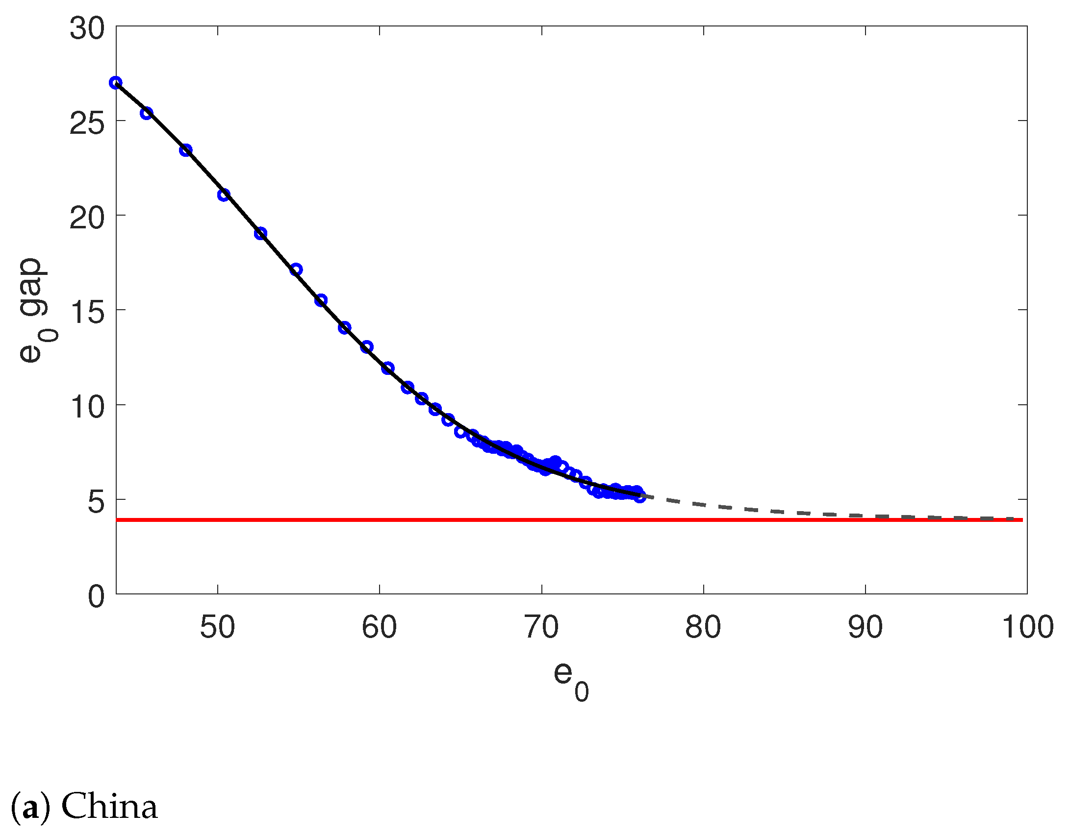
In Figure 2, we plot the life expectancy gap with respect to the benchmark life expectancy defined in Equation (8) against the life expectancy level in the same period for 149 less developed countries5. First, we can see that the life expectancy gap tends to decrease as the life expectancy level increases. Second, and more importantly, the speed of decline depends non-linearly on the life expectancy level, which echoes the aforementioned discussion. Specifically, the average decrease in the life expectancy gap is slow before the life expectancy reaches 45; it accelerates when the life expectancy increases to between 45 and 70 and slows down again after the life expectancy exceeds 70. Hence, as the life expectancy level of a less developed country further increases, the gap is likely to continue to narrow for a certain period and become stable in the long term.
In fact, the aforementioned relationship between and can be fitted by the double logistic function:
where and are normalization coefficients, and is the vector of unknown parameters to be estimated. The double logistic function has previously been used by the United Nations (Raftery et al. 2013) to capture the relationship between the growth and the level of the life expectancy in different countries and periods6. It allows to decline with decreasing speed, and finally converge to a long-term mean characterized by . Equation (14) can be fitted by minimizing the squared residuals of the observed and the fitted life expectancy gaps. For further discussion of the double logistic function in the modeling of life expectancy, see Raftery et al. (2013) and Castanheira et al. (2017). The double logistic function is applied to the 50% quantile of the life expectancy gap (the solid line in Figure 2) and provides a very good fit.
In general, not all less developed countries require a double logistic function to fit their life expectancy gaps. In this case, we could use the simpler single logistic regression model for the life expectancy gap:
Therefore, we need to first determine which logistic function is more suitable for a less developed country. This can be done using information criteria such as the AIC and the BIC ratios.
4. Empirical Analysis
In this section, we apply the rotation algorithm to three less developed countries, China, Brazil, and Nigeria, which are the most populous countries in their respective continents. First, we introduce the data used in the analysis, and then we discuss the empirical results for each country.
4.1. Mortality Data
We use 10 more developed countries to construct the benchmark: Germany, Denmark, Finland, France, The Netherlands, Switzerland, Sweden, the UK, the US, and Japan. The unisex mortality rates of these countries were downloaded from the Human Mortality Database (HMD)7. In particular, we use the central death rates in the 5-age and 1-year blocks, i.e., 0–4, 5–9, …, 95–99, and from 1960 to 2015.
Mortality data for the three less developed countries are not included in the HMD and were thus obtained from two other sources: the Population Division of the United Nations (UN) and the World Health Organization (WHO)8. The UN dataset covers the death counts and the corresponding exposures for a longer period (1960–2015), but the data are divided into 5-year blocks. On the other hand, the WHO dataset contains more granular death counts and exposures in 1-year blocks, but covers a shorter period, between 2000 and 2015. Moreover, the age groups are 0–4, 5–9, …, 80+ for the UN data, and 0, 1–4, …, 85+ for the WHO data.
In order to extract as much information as possible from the UN and WHO data, we merge these two datasets in a format compatible with the mortality data of the 10 benchmark countries. The merged dataset contains the central death rates in 5-age and 1-year blocks, with age groups 0–4, 5–9, …, 95–99 from 1960 to 2015. Technical details are gathered in the Appendix of Li et al. (2018). Finally, we remark that the proposed rotation algorithm is not only applicable to the forecasting of national mortality data but also to life insurance and pension risk management applications, such as those considered in Li et al. (2017), Li (2018), and Chen et al. (2021).
4.2. Empirical Results
We first determine the optimal logistic function for each of the three countries. In particular, we find that the single logistic function is optimal for China, whereas the double logistic function is more suitable for Brazil and Nigeria. The AIC and BIC ratios for both regressions fitted to each of the three countries are presented in Appendix A.
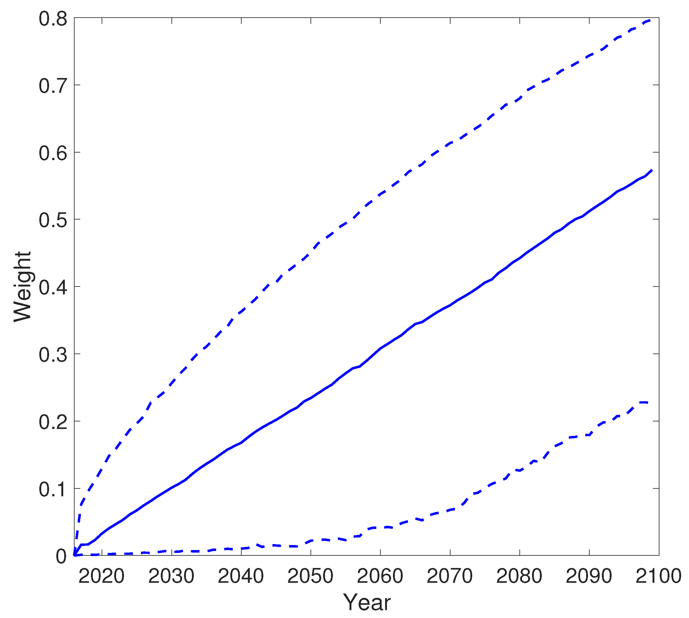
Figure 3 shows the actual, fitted, and predicted future life expectancy gap for the three countries along with the respective optimal logistic function. We see that the logistic functions give reasonably good fits for China and Brazil. For Nigeria, the observed life expectancy gap has a jump around , which results from the stagnation of its life expectancy at birth in the 1990s. Although the double logistic function is not able to capture this jump, it gives a satisfactory fit on the general decreasing pattern. By extrapolating the logistic functions, we obtain a of 3.9 years for China, 5.6 years for Brazil, and 3.9 years for Nigeria. The results of the three countries are plotted as horizontal lines in the figures. Using these values, the expected completion time of the rotation algorithm is 2022 for China and 2029 for Brazil. For Nigeria, however, the rotation is not completed by 2100 (with the 50% quantile of the being 0.58). The weights for the three countries are shown in Appendix B. Let us now turn to the historical mortality patterns, the projected age-specific mortality rates, and the remaining life expectancy at 65 for each country. In particular, we simulate 2500 paths to produce the projections by the rotation algorithm to compute the life expectancy. The projected life expectancy at birth for the three countries shows qualitatively similar patterns to the remaining life expectancy at 65, and these are presented in Appendix C.
4.2.1. China
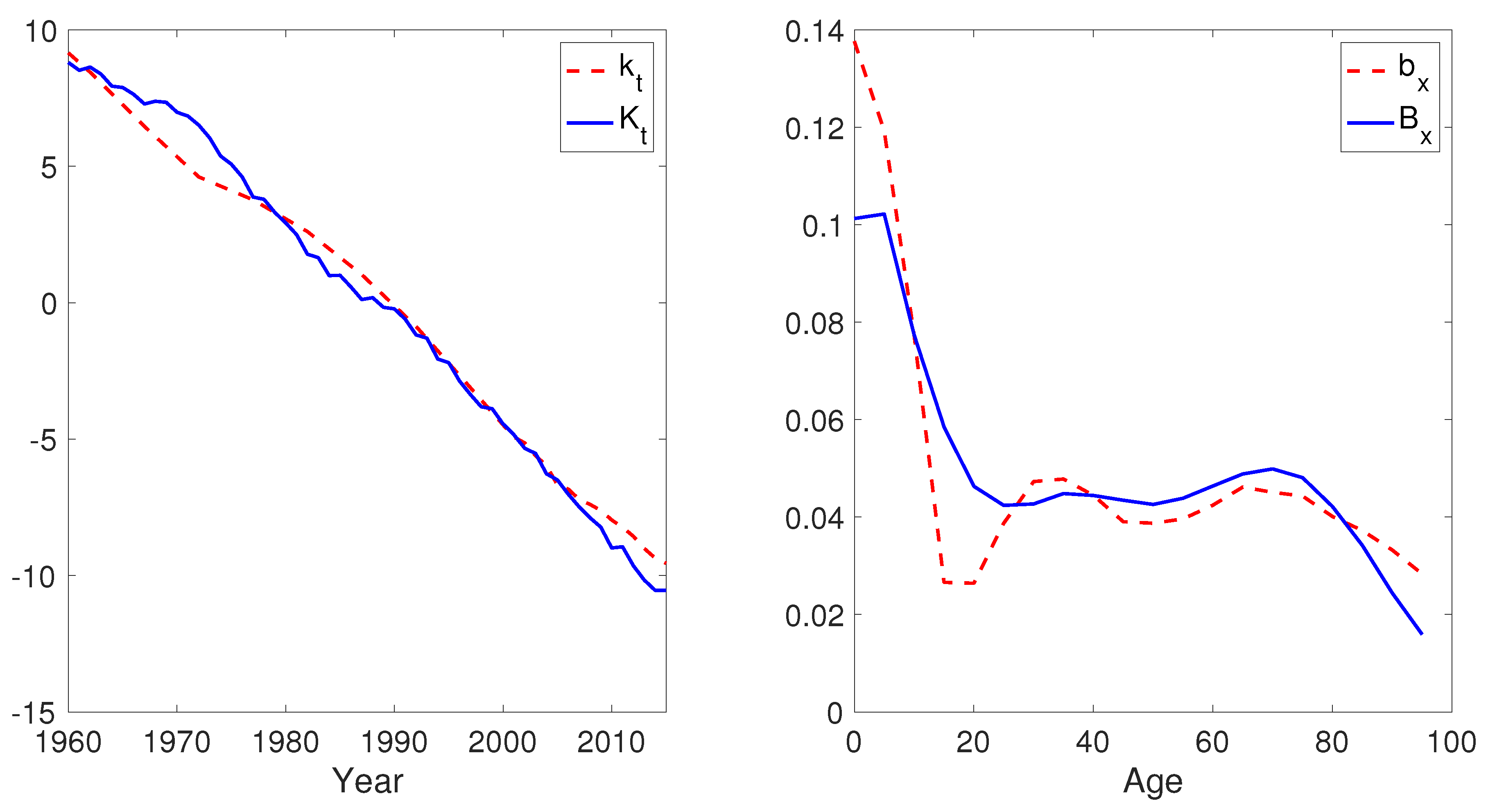
Figure 4 plots the period and the age effects of China ( and ) and of the benchmark countries ( and ). We see that is rather close to linear, but has a non-linear pattern over the sample period. Specifically, declines drastically between 1960 and 1975, flattens between 1975 and 1995, and then resumes the steep decreasing trend afterwards. Therefore, the assumption of the random walk with constant drift is clearly not appropriate for China. Moreover, is decreasing in x, indicating faster historical mortality improvement rates among the younger ages. In particular, China’s age effects are substantially lower for the old ages than the benchmark values.
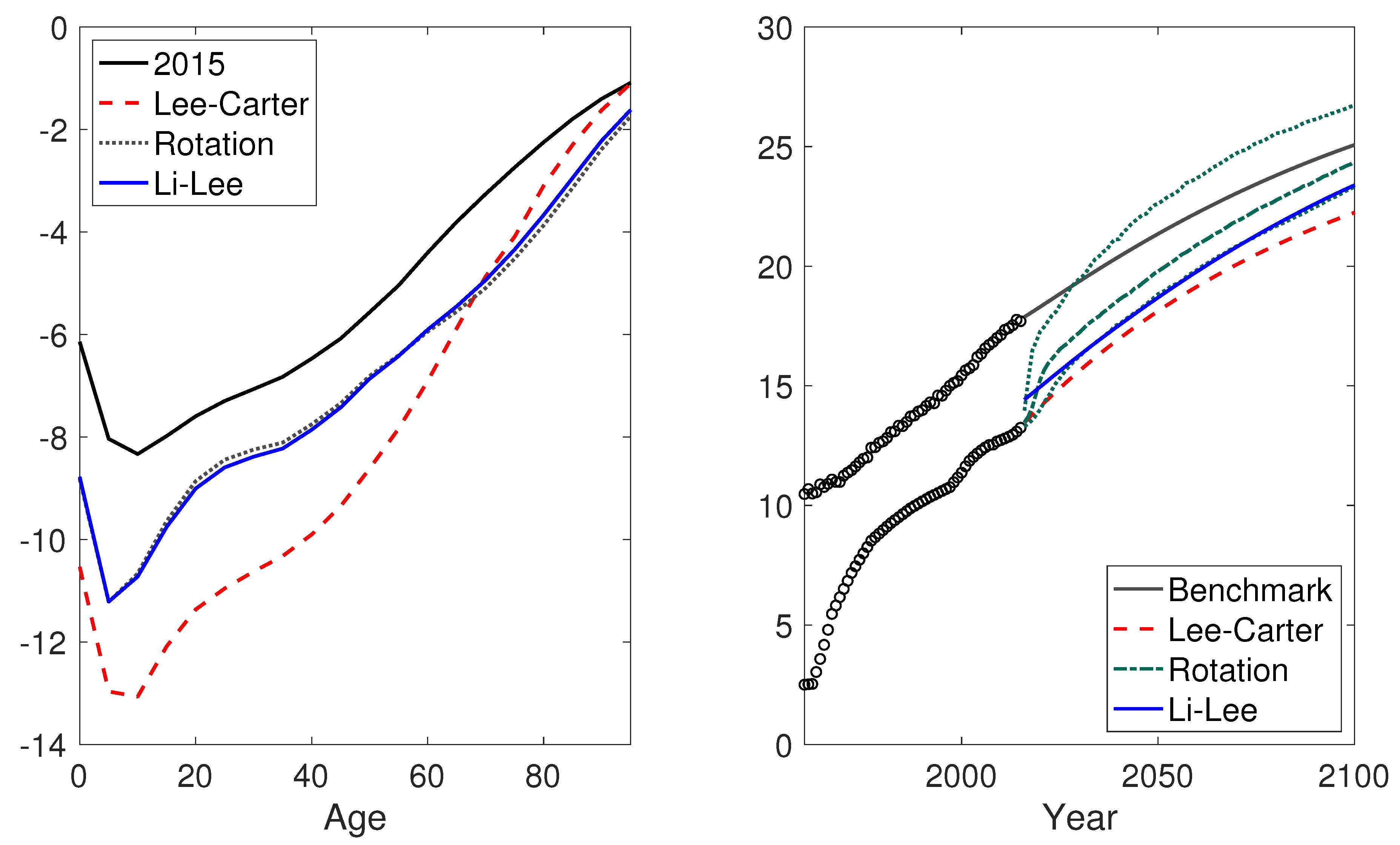
Figure 5 shows the projected mortality differential between China and the benchmark countries, both in terms of the logarithm age-specific death rates (left panel) and the remaining life expectancy at 65 (right panel). First, the left panel compares the observed and the projected 50% quantile of the from the independent Lee–Carter model, the Li–Lee model, and the rotation algorithm, respectively. We see that the independent Lee–Carter model leads to a more substantial aggregate mortality decline and, more importantly, rather imbalanced mortality improvements across ages. In particular, while the mortality declines are huge at younger ages, they are projected to be very limited among the elders. In contrast, the projected values of the Li–Lee model and the rotation algorithm are rather similar and are much more balanced across ages.
Meanwhile, the rotation algorithm leads to a projected that is 2.2 years higher than that of the Lee–Carter model (24.4 vs. 22.2). Moreover, while the Li–Lee model produces rather similar values to the rotation algorithm, its projected is significantly different (0.7 years lower than the rotation algorithm). The reason is that, due to the imposition of instant coherence, the Li–Lee model generates different age-specific mortality rates to the rotation algorithm in the early phase of the projection (before the rotation is finished). Such differences will be reflected in the projected life expectancy and carried over to the long term.
4.2.2. Brazil
From Figure 6, we see that the historical period effect of Brazil is very similar to the benchmark values, especially since 1990. However, the values are substantially lower than the values for the teenage and young ages (10 to 25), and higher for infants and the very old ages. One possible reason for the low values is the high historical violence-related mortality rates of young people in the South and Central American countries (Viner et al. 2011).
Figure 7 suggests that the values projected by the independent Lee–Carter model are indeed much higher than those of the rotation model from age 10 to 25. Moreover, the projected is 0.6 years higher when the rotation algorithm is used (23.7 vs. 23.1). Our rotation algorithm yields similar projection results, as the mortality patterns of Brazil are different from the benchmark values for only a few ages. On the contrary, Li–Lee model is not applicable in this case, given the fact that the autocorrelation coefficient ( in Equation (5)) is 1.03 under the Li–Lee model when and are imposed.
4.2.3. Nigeria
For Nigeria, we see from Figure 8 that the is not only much flatter than but also rather non-linear. Moreover, the values are rather irregular, with substantially higher values for ages 0–4 and 15–30, and lower values for ages above 60 than .
Meanwhile, the projected values displayed in Figure 9 are lower under the rotation algorithm than the independent Lee–Carter model, except for infants and ages around 30. Moreover, the rotation algorithm gives much higher projected than the independent Lee–Carter model (12.4 vs. 9.8). The mortality projections of Nigeria are significantly different to those of China and Brazil. The most important reason is that the historical mortality level of Nigeria was comparatively low, and its life expectancy was much lower than that of the benchmark mortality. Specifically, although the double logistic function projects a very low , it is far from being reached in 2100 based on the large historical life expectancy gap. As a result, the weight of the Li–Lee model was relatively low in the projection phase, and the (low) historical mortality improvement of Nigeria still exerts a dominant effect on the projection, which results in a low projected mortality level in 2100. Similarly, its projected is still substantially lower than that of China and Brazil. Finally, similar to Brazil, the autocorrelation coefficient is larger than 1 (1.09) for Nigeria; thus, the Li–Lee projections are not feasible.
5. Conclusions
This paper has proposed a mortality rotation approach for the coherent forecasting of age-specific mortality rates in the less developed countries. While the historical mortality patterns of these countries are generally different from the more developed ones, such discrepancies are likely to diminish along with future socioeconomic developments. Our approach incorporates the future changes in mortality patterns for the less developed countries in the projection phase. In particular, we allow the mortality patterns of a less developed country to be weighted averages of its own historical patterns and the benchmark patterns derived from a set of more developed countries. The weights of the benchmark values start from 0 and gradually increase to 1 as the projected life expectancy gap between the less developed country and the benchmark more developed countries decreases. Finally, coherence is achieved when the projected life expectancy gap reaches a lower threshold. In our analysis, we allow the threshold to be the long-term life expectancy gap between the less developed country and the benchmark countries. This long-term gap is projected by a logistic function of the historical life expectancy gaps on the life expectancy levels.
The rotation approach is applied to China, Brazil, and Nigeria, the most populous countries in Asia, South America, and Africa, respectively. We show that the rotation algorithm is applicable to countries that exhibit significantly different mortality experience to the benchmark developed countries (Brazil and Nigeria), where the projections of the Li–Lee model are not feasible. Moreover, the rotation algorithm produces more intuitive projections of age-specific mortality rates and life expectancy than the independent forecasts of the Lee–Carter model.
There are a couple interesting possible extensions of the current work. First, in this research, we have applied the Li–Lee model, which has time-invariant age effects, to the benchmark mortality. As noted by many studies (see, for example, Li and Shi 2021a; Li et al. 2013), the Li–Lee model will generate divergent mortality forecasts among ages. In future research, it would be interesting to consider a rotation algorithm, such as the one considered in Li et al. (2013), in addition to the Li–Lee model. In this way, the age-specific mortality projections of the benchmark mortality themselves would be coherent in the long run. Second, this research only considers three less developed countries. It would be interesting to apply the proposed rotation algorithm to additional less developed countries, such as those in Europe and North America.
Author Contributions
Methodology, H.L. and P.L.; formal analysis, H.L. and P.L.; writing—original draft preparation, H.L., Y.L. and P.L.; writing—review and editing, H.L., Y.L. and P.L.; visualization, H.L. and P.L. All authors have read and agreed to the published version of the manuscript.
Funding
This research was funded by the Society of Actuaries (Modeling and Forecasting Chinese Population Dynamics in a Multi-population Context), and the Natural Sciences and Engineering Research Council of Canada (NSERC), (RGPIN-2020-05387) and (DGECR-2020-00347).
Data Availability Statement
Mortality data of the developed countries are obtained from the Human Mortality Database (HMD)9. Mortality data of the less developed countries are obtained from two sources: the Population Division of the United Nations (UN) and the World Health Organization (WHO)10. All databases are publicly available.
Conflicts of Interest
The authors declare no conflict of interest.
Abbreviations
The following abbreviations and variables are used in this manuscript:
| Variables of the Lee–Carter model: | |
| Log central mortality rate at age x in year t | |
| The average mortality level at each age x | |
| The mortality index at time t | |
| The age-specific sensitivity of to changes in | |
| The normal error term in the process | |
| The normal error term in the process | |
| Additional variables of the Li–Lee models | |
| Age effect of the common factor | |
| Period effect of the common factor | |
| The normal error term in the common factor | |
| The age-specific sensitivity of log central mortality rate to the population-specific index | |
Appendix A. Optimal Logistic Function
We determine the optimal (single or double) logistic function for China, Brazil, and Nigeria, using the Akaike information criterion (AIC) and Bayesian information criterion (BIC). More specifically, the AIC and BIC ratios are given by the corresponding equations:
and
where k is the number of free parameters, N is the size of the sample, and is the log-likelihood of the model. The AIC and BIC ratios select the best model by balancing the number of free parameters and the in-sample fit of the model. In particular, a lower BIC or AIC indicates a better model.
For each country, we fit the double and the single logistic function (Equations (14) and (15) in the paper) of its life expectancy gap to the life expectancy level . The corresponding AIC and BIC ratios are gathered in Table A1. Both the AIC and BIC ratios suggest that the single logistic function is optimal for China, while the double logistic function is optimal for Brazil and Nigeria.

Table A1.
The AIC and the BIC ratios of the single and the double logistic function of the life expectancy gap for China, Brazil, and Nigeria. The lowest values of AIC and BIC for each country are marked in bold.
Table A1.
The AIC and the BIC ratios of the single and the double logistic function of the life expectancy gap for China, Brazil, and Nigeria. The lowest values of AIC and BIC for each country are marked in bold.
| AIC | ||
| Country | Single logistic | Double logistic |
| China | −21.32 | −16.23 |
| Brazil | 40.68 | −13.75 |
| Nigeria | 154.14 | 140.36 |
| BIC | ||
| Country | Single logistic | Double logistic |
| China | −13.22 | |
| Brazil | 48.79 | 0.43 |
| Nigeria | 162.24 | 154.54 |
Appendix B. The Weight Parameter of the Rotation Algorithm
In this appendix, we show the simulated weights in the rotation algorithm for China, Brazil, and Nigeria, following the simulation procedure in the section “The rotation algorithm”.
As shown in Figure A1, approaches 1 in 2020 on average for China. Meanwhile, the 97.5% quantile of reaches 1 in 2018, while the 2.5% quantile is much lower and ends at around 0.65 in 2100.
Figure A1.
The 2.5%, 50%, and 97.5% quantile of the weight over time for China.

As for Brazil, Figure A2 shows that the median rotation completion time is 2029. Moreover, it is completed by 2040 in 97.5% of the simulated scenarios, and before 2020 in 2.5% of the scenarios. The 95% confidence bound of for Brazil is narrower than that of China, indicating that Brazil’s historical mortality experience is less volatile.
Figure A2.
The 2.5%, 50%, and 97.5% quantile of the weight over time for Brazil.

Figure A3 shows that the rotation for Nigeria has, on average, not yet finished by the end of the projection phase. In 2100, becomes 0.58 on average, and it becomes 0.8 (resp. 0.22) for the 97.5% (resp. 2.5%) quantile.
Figure A3.
The 2.5%, 50%, and 97.5% quantile of the weight over time for Nigeria.

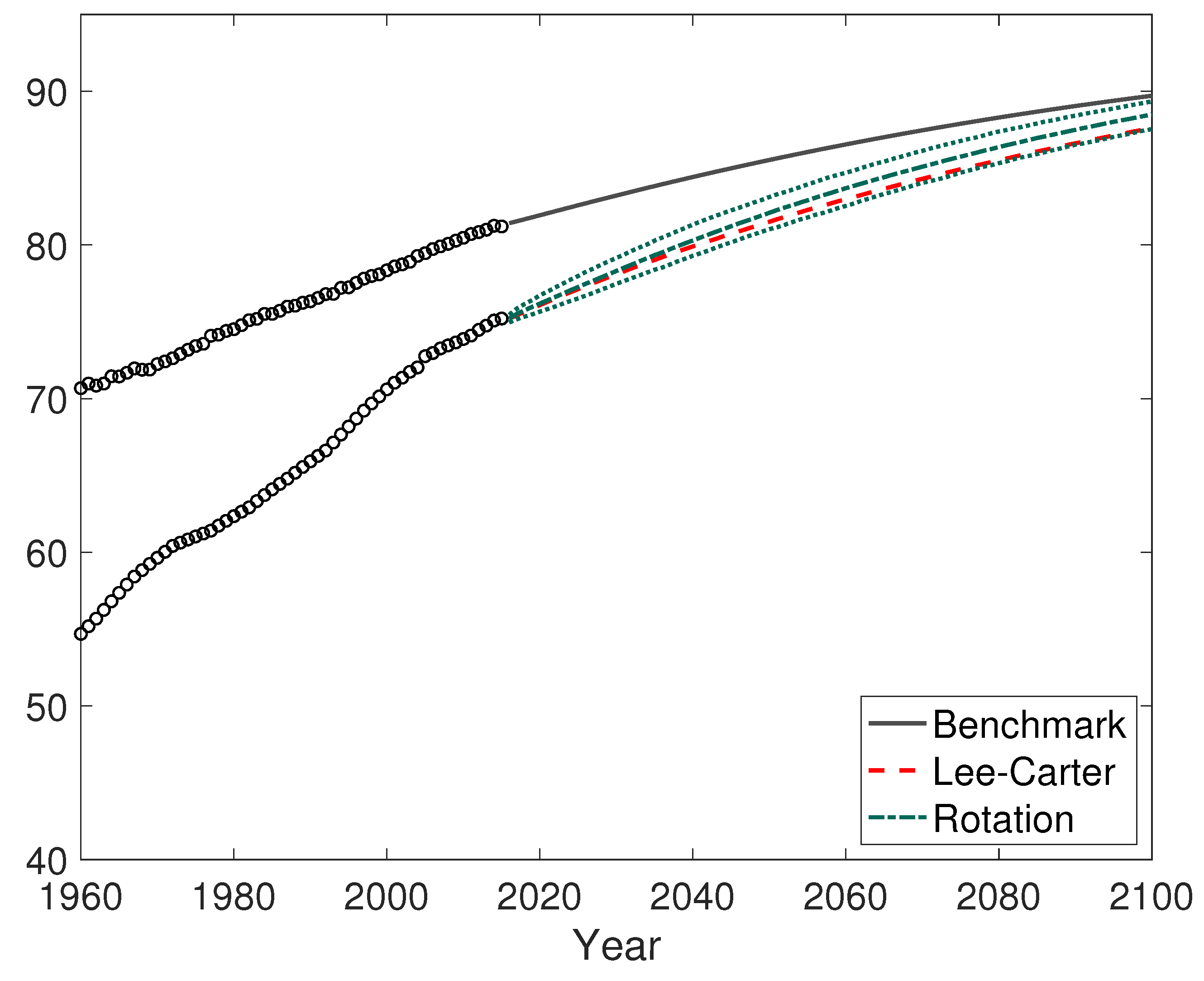
Appendix C. The Projected Life Expectancy at Birth
The projected life expectancies at birth of China, Brazil, and Nigeria are plotted in Figure A4, Figure A5 and Figure A6, respectively. In each figure, the average projected life expectancy of the 10 benchmark countries is also shown.
Figure A4.
The average projected life expectancy of the benchmark countries and China using the rotation algorithm and the independent Lee–Carter model.
Figure A4.
The average projected life expectancy of the benchmark countries and China using the rotation algorithm and the independent Lee–Carter model.

Figure A5.
The average projected life expectancy of the benchmark countries and Brazil using the rotation algorithm and the independent Lee–Carter model.
Figure A5.
The average projected life expectancy of the benchmark countries and Brazil using the rotation algorithm and the independent Lee–Carter model.

Figure A6.
The average projected life expectancy of the benchmark countries and Nigeria using the rotation algorithm and the independent Lee–Carter model.
Figure A6.
The average projected life expectancy of the benchmark countries and Nigeria using the rotation algorithm and the independent Lee–Carter model.

| 1 | The United Nations defines the less developed countries/regions as all regions of Africa, Asia (except Japan), Latin America and the Caribbean plus Melanesia, Micronesia and Polynesia, and the more developed countries/regions as all regions in Europe, Northern America, Australia, New Zealand, and Japan. For ease of exposition, we will use the word “country” to refer to any country or region. |
| 2 | The age-specific death rates are calculated using data from the 2017 revision of the World Population Prospects by the United Nations. The ranking is based on population statistics as of 1 June 2018. Source: https://www.census.gov/popclock/print.php?component=counter (accessed on 14 August 2021). |
| 3 | Besides these two models, there are many other linear extrapolation models consistent with our rotation algorithm, such as Cairns et al. (2006) and Hyndman and Ullah (2007), as well as Li et al. (2021) for a single population and Dowd et al. (2011), Hyndman et al. (2013), Li et al. (2019), Li and Lu (2018, 2019) for multiple populations. For summaries of linear extrapolation models, we refer to Booth et al. (2002), Cairns et al. (2011), and Li and Hardy (2011). |
| 4 | When convergence is achieved, the improvement rates of the logarithm of the age-specific mortality rates are the same between the modeled country and the benchmark countries. However, this does not necessarily lead to the same improvement rate of the life expectancy, due to Jensen’s inequality. |
| 5 | The data were collected from the 2017 revision of the World Population Prospects. We excluded 9 less developed countries/regions with life expectancy higher than 80 in 2010–2015, such as Hong Kong, Macao, and Singapore. The benchmark life expectancy was calculated using 10 more developed countries: Germany, Denmark, Finland, France, The Netherlands, Switzerland, Sweden, the UK, the US, and Japan. |
| 6 | The United Nations uses a simplified version of Equation (14) where is set to 0. |
| 7 | Source: http://www.mortality.org/ (accessed on 14 August 2021). |
| 8 | UN Source: http://www.un.org/en/development/desa/population/ (accessed on 14 August 2021). WHO Source: http://apps.who.int/gho/data/view.main.60340?lang=en (accessed on 14 August 2021). |
| 9 | Source: http://www.mortality.org/ (accessed on 14 August 2021). |
| 10 | UN Source: http://www.un.org/en/development/desa/population/ (accessed on 14 August 2021). WHO Source: http://apps.who.int/gho/data/view.main.60340?lang=en (accessed on 14 August 2021). |
References
- Abegunde, Dele O., Colin D. Mathers, Taghreed Adam, Monica Ortegon, and Kathleen Strong. 2007. The burden and costs of chronic diseases in low-income and middle-income countries. The Lancet 370: 1929–38. [Google Scholar] [CrossRef]
- Andreev, Kirill, and James Vaupel. 2006. Forecasts of cohort mortality after age 50. In Max Planck Institute for Demographic Research Working Paper. Rostock: Max Planck Institute for Demographic Research, vol. 12. [Google Scholar]
- Austin, Kelly, and Laura McKinney. 2012. Disease, war, hunger, and deprivation: A cross-national investigation of the determinants of life expectancy in less-developed and sub-saharan african nations. Sociological Perspectives 55: 421–47. [Google Scholar] [CrossRef]
- Booth, Heather, John Maindonald, and Len Smith. 2002. Applying Lee-Carter under conditions of variable mortality decline. Population Studies 56: 325–36. [Google Scholar] [CrossRef]
- Cairns, Andrew, David Blake, and Kevin Dowd. 2006. A two-factor model for stochastic mortality with parameter uncertainty: Theory and calibration. Journal of Risk and Insurance 73: 687–718. [Google Scholar] [CrossRef]
- Cairns, Andrew, David Blake, Kevin Dowd, Guy Coughlan, David Epstein, and Marwa Khalaf-Allah. 2011. Mortality Density Forecasts: An Analysis of Six Stochastic Mortality Models. Insurance: Mathematics and Economics 48: 355–67. [Google Scholar] [CrossRef] [Green Version]
- Cairns, Andrew J. G., David Blake, Kevin Dowd, Guy D. Coughlan, David Epstein, Alen Ong, and Igor Balevich. 2009. A quantitative comparison of stochastic mortality models using data from england and wales and the united states. North American Actuarial Journal 13: 1–35. [Google Scholar] [CrossRef]
- Castanheira, Helena, François Pelletier, and Igor Ribeiro. 2017. A Sensitivity Analysis of the Bayesian Framework for Projecting Life Expectancy at Birth. In UN Population Division. Technical Paper. New York: United Nations, No. 7. [Google Scholar]
- Chen, An, Hong Li, and Mark Schultze. 2021. Tail index-linked annuity: A longevity risk sharing retirement plan. Scandinavian Actuarial Journal. [Google Scholar] [CrossRef]
- CMI. 2009. Continuous Mortality Investigation: A Prototype Mortality Projections Model: Part Two—Detailed Analysis. Working Paper. London: Institute and Faculty of Actuaries, No. 39. [Google Scholar]
- Dowd, Kevin, Andrew Cairns, David Blake, Guy Coughlan, and Marwa Khalaf-Allah. 2011. A gravity model of mortality rates for two related populations. North American Actuarial Journal 15: 334–56. [Google Scholar] [CrossRef] [Green Version]
- Fogel, Robert. 2004. The Escape from Hunger and Premature Death, 1700–2100: Europe, America, and the Third World. Cambridge: Cambridge University Press, vol. 38. [Google Scholar]
- Hensher, Martin, Max Price, and Sarah Adomakoh. 2017. Disease Control Priorities in Developing Countries. Oxford: Oxford University Press. [Google Scholar]
- Huang, Fei, and Bridget Browne. 2017. Mortality forecasting using a modified continuous mortality investigation mortality projections model for china i: Methodology and country-level results. Annals of Actuarial Science 11: 20–45. [Google Scholar] [CrossRef]
- Hyndman, Rob J., Heather Booth, and Farah Yasmeen. 2013. Coherent mortality forecasting: The product-ratio method with functional time series models. Demography 50: 261–83. [Google Scholar] [CrossRef] [Green Version]
- Hyndman, Rob J., and Md Shahid Ullah. 2007. Robust forecasting of mortality and fertility rates: A functional data approach. Computational Statistics & Data Analysis 51: 4942–56. [Google Scholar]
- Jeuland, Marc A., David E. Fuente, Semra Ozdemir, Maura C. Allaire, and Dale Whittington. 2013. The long-term dynamics of mortality benefits from improved water and sanitation in less developed countries. PLoS ONE 8: e74804. [Google Scholar] [CrossRef] [Green Version]
- Lee, Ronald, and Timothy Miller. 2001. Evaluating the performance of the lee-carter method for forecasting mortality. Demography 38: 537–49. [Google Scholar] [CrossRef]
- Lee, Ronald, and Lawrence R. Carter. 1992. Modeling and forecasting US mortality. Journal of the American Statistical Association 87: 659–71. [Google Scholar]
- Li, Hong. 2018. Dynamic hedging of longevity risk: The effect of trading frequency. ASTIN Bulletin: The Journal of the IAA 48: 197–232. [Google Scholar] [CrossRef]
- Li, Hong, Anja De Waegenaere, and Bertrand Melenberg. 2015. The choice of sample size for mortality forecasting: A bayesian learning approach. Insurance: Mathematics and Economics 63: 153–68. [Google Scholar] [CrossRef]
- Li, Hong, Anja De Waegenaere, and Bertrand Melenberg. 2017. Robust mean–variance hedging of longevity risk. Journal of Risk and Insurance 84: 459–75. [Google Scholar] [CrossRef]
- Li, Han, Hong Li, Yang Lu, and Anastasios Panagiotelis. 2019. A forecast reconciliation approach to cause-of-death mortality modeling. Insurance: Mathematics and Economics 86: 122–33. [Google Scholar] [CrossRef]
- Li, Hong, and Johnny S. H. Li. 2017. Optimizing the Lee-Carter Approach in the Presence of Structural Changes in Time and Age Patterns of Mortality Improvements. Demography 54: 1073–95. [Google Scholar] [CrossRef] [PubMed]
- Li, Hong, and Yang Lu. 2017. Coherent forecasting of mortality rates: A sparse vector-autoregression approach. ASTIN Bulletin: The Journal of the IAA 47: 563–600. [Google Scholar] [CrossRef]
- Li, Hong, and Yang Lu. 2018. A bayesian non-parametric model for small population mortality. Scandinavian Actuarial Journal 2018: 605–28. [Google Scholar] [CrossRef]
- Li, Hong, and Yang Lu. 2019. Modeling cause-of-death mortality using hierarchical archimedean copula. Scandinavian Actuarial Journal 2019: 247–72. [Google Scholar] [CrossRef]
- Li, Hong, Yang Lu, and Pintao Lyu. 2018. Modeling and forecasting chinese population dynamics in a multi-population context. In SOA Research Reports. Schaumburg: Society of Actuaries. [Google Scholar]
- Li, Hong, and Yanlin Shi. 2021a. Forecasting mortality with international linkages: A global vector-autoregression approach. Insurance: Mathematics and Economics 100: 59–75. [Google Scholar] [CrossRef]
- Li, Hong, and Yanlin Shi. 2021b. Mortality forecasting with an age-coherent sparse var model. Risks 9: 35. [Google Scholar] [CrossRef]
- Li, Hong, Ken Seng Tan, Shripad Tuljapurkar, and Wenjun Zhu. 2021. Gompertz law revisited: Forecasting mortality with a multi-factor exponential model. Insurance: Mathematics and Economics 99: 268–81. [Google Scholar] [CrossRef]
- Li, Johnny S. H., and Mary Hardy. 2011. Measuring basis risk in longevity hedges. North American Actuarial Journal 15: 177–200. [Google Scholar] [CrossRef]
- Li, Nan, and Ronald D. Lee. 2005. Coherent mortality forecasts for a group of populations: An extension of the Lee-Carter method. Demography 42: 575–94. [Google Scholar] [CrossRef] [Green Version]
- Li, Nan, Ronald Lee, and Patrick Gerland. 2013. Extending the Lee-Carter method to model the rotation of age patterns of mortality decline for long-term projections. Demography 50: 2037–51. [Google Scholar] [CrossRef] [Green Version]
- Lin, Ro-Ting, Ya-Mei Chen, Lung-Chang Chien, and Chang-Chuan Chan. 2012. Political and social determinants of life expectancy in less developed countries: A longitudinal study. BMC Public Health 12: 85. [Google Scholar] [CrossRef] [Green Version]
- Lutz, Wolfgang, Warren Sanderson, and Sergei Scherbov. 2008. The coming acceleration of global population ageing. Nature 451: 716. [Google Scholar] [CrossRef]
- Mensah, George A., Gina S. Wei, Paul D. Sorlie, Lawrence J. Fine, Yves Rosenberg, Peter G. Kaufmann, Michael E. Mussolino, Lucy L. Hsu, Ebyan Addou, Michael M. Engelgau, and et al. 2017. Decline in cardiovascular mortality: Possible causes and implications. Circulation Research 120: 366–80. [Google Scholar] [CrossRef] [PubMed]
- Müller, Olaf, and Michael Krawinkel. 2005. Malnutrition and health in developing countries. Canadian Medical Association Journal 173: 279–86. [Google Scholar] [CrossRef] [Green Version]
- Peto, Richard, J. Boreham, Alan D. Lopez, Michael Thun, and Clark Heath. 1992. Mortality from tobacco in developed countries: Indirect estimation from national vital statistics. The Lancet 339: 1268–78. [Google Scholar] [CrossRef]
- Raftery, Adrian E., Jennifer L. Chunn, Patrick Gerland, and Hana Ševčíková. 2013. Bayesian probabilistic projections of life expectancy for all countries. Demography 50: 777–801. [Google Scholar] [CrossRef] [PubMed] [Green Version]
- Renshaw, Arthur E., and Steven Haberman. 2006. A cohort-based extension to the lee–carter model for mortality reduction factors. Insurance: Mathematics and Economics 38: 556–70. [Google Scholar] [CrossRef]
- Riley, James. C. 2001. Rising Life Expectancy: A Global History. Cambridge: Cambridge University Press. [Google Scholar]
- Torri, Tiziana, and James W. Vaupel. 2012. Forecasting life expectancy in an international context. International Journal of Forecasting 28: 519–31. [Google Scholar] [CrossRef]
- Tuljapurkar, Shripad, Nan Li, and Carl Boe. 2000. A universal pattern of mortality decline in the G7 countries. Nature 405: 789. [Google Scholar] [CrossRef]
- United Nations. 2017. World Population Prospects: The 2017 Revision. New York: United Nations. [Google Scholar]
- Viner, Russell, Carolyn Coffey, Colin Mathers, Paul Bloem, Anthony Costello, John Santelli, and George Patton. 2011. 50-year mortality trends in children and young people: A study of 50 low-income, middle-income, and high-income countries. The Lancet 377: 1162–74. [Google Scholar] [CrossRef]
Figure 1.
The logarithm of the age-specific central death rates for the five most populous countries, China, India, the US, Indonesia, and Brazil, in 1960 (left panel) and 2015 (right panel).
Figure 1.
The logarithm of the age-specific central death rates for the five most populous countries, China, India, the US, Indonesia, and Brazil, in 1960 (left panel) and 2015 (right panel).

Figure 2.
Life expectancy gaps against the life expectancy level for the less developed countries (in grey dots), the 50% quantile (dashed line), and the smoothed fit by the double logistic function (solid line).
Figure 2.
Life expectancy gaps against the life expectancy level for the less developed countries (in grey dots), the 50% quantile (dashed line), and the smoothed fit by the double logistic function (solid line).

Figure 3.
The observed, fitted, and predicted life expectancy gaps for China, Brazil, and Nigeria using their respective optimal logistic function.
Figure 3.
The observed, fitted, and predicted life expectancy gaps for China, Brazil, and Nigeria using their respective optimal logistic function.


Figure 4.
The historical period effects (left panel) and the age effects (right panel) of China and the benchmark populations.
Figure 4.
The historical period effects (left panel) and the age effects (right panel) of China and the benchmark populations.

Figure 5.
The projected logarithm age-specific death rates (left panel) and the remaining life expectancy at 65 (right panel) of the average of the benchmark countries and China using different models. For the rotation algorithm, the 2.5%, 50%, and 97.5% quantile of the projected are plotted.
Figure 5.
The projected logarithm age-specific death rates (left panel) and the remaining life expectancy at 65 (right panel) of the average of the benchmark countries and China using different models. For the rotation algorithm, the 2.5%, 50%, and 97.5% quantile of the projected are plotted.

Figure 6.
The historical period effects (left panel) and the age effects (right panel) of Brazil and the benchmark populations.
Figure 6.
The historical period effects (left panel) and the age effects (right panel) of Brazil and the benchmark populations.

Figure 7.
The projected logarithm age-specific death rates (left panel) and the remaining life expectancy at 65 (right panel) of the average of the benchmark countries and Brazil using different models. For the rotation algorithm, the 2.5%, 50%, and 97.5% quantile of the projected are plotted.
Figure 7.
The projected logarithm age-specific death rates (left panel) and the remaining life expectancy at 65 (right panel) of the average of the benchmark countries and Brazil using different models. For the rotation algorithm, the 2.5%, 50%, and 97.5% quantile of the projected are plotted.

Figure 8.
The historical period effects (left panel) and the age effects (right panel) of Nigeria and the benchmark populations.
Figure 8.
The historical period effects (left panel) and the age effects (right panel) of Nigeria and the benchmark populations.

Figure 9.
The projected logarithm age-specific death rates (left panel) and the remaining life expectancy at 65 (right panel) of the average of the benchmark countries and Nigeria using different models. For the rotation algorithm, the 2.5%, 50%, and 97.5% quantile of the projected are plotted.
Figure 9.
The projected logarithm age-specific death rates (left panel) and the remaining life expectancy at 65 (right panel) of the average of the benchmark countries and Nigeria using different models. For the rotation algorithm, the 2.5%, 50%, and 97.5% quantile of the projected are plotted.

Publisher’s Note: MDPI stays neutral with regard to jurisdictional claims in published maps and institutional affiliations. |
© 2021 by the authors. Licensee MDPI, Basel, Switzerland. This article is an open access article distributed under the terms and conditions of the Creative Commons Attribution (CC BY) license (https://creativecommons.org/licenses/by/4.0/).
Share and Cite
MDPI and ACS Style
Li, H.; Lu, Y.; Lyu, P. Coherent Mortality Forecasting for Less Developed Countries. Risks 2021, 9, 151. https://doi.org/10.3390/risks9090151
AMA Style
Li H, Lu Y, Lyu P. Coherent Mortality Forecasting for Less Developed Countries. Risks. 2021; 9(9):151. https://doi.org/10.3390/risks9090151
Chicago/Turabian StyleLi, Hong, Yang Lu, and Pintao Lyu. 2021. "Coherent Mortality Forecasting for Less Developed Countries" Risks 9, no. 9: 151. https://doi.org/10.3390/risks9090151
Note that from the first issue of 2016, this journal uses article numbers instead of page numbers. See further details here.