Modelling Australian Dollar Volatility at Multiple Horizons with High-Frequency Data


1
Economics Department, Business School, The University of Western Australia, Crawley, WA 6009, Australia
2
Faculty of Finance, Banking and Business Administration, Quy Nhon University, Binh Dinh 560000, Vietnam
3
Business and Economics Research Group, Ho Chi Minh City Open University, Ho Chi Minh City 7000, Vietnam
*
Author to whom correspondence should be addressed.
Risks 2020, 8(3), 89; https://doi.org/10.3390/risks8030089
Submission received: 1 July 2020
/
Revised: 14 August 2020
/
Accepted: 17 August 2020
/
Published: 26 August 2020
(This article belongs to the Special Issue Quantitative Methods in Economics and Finance)
Abstract
:Long-range dependency of the volatility of exchange-rate time series plays a crucial role in the evaluation of exchange-rate risks, in particular for the commodity currencies. The Australian dollar is currently holding the fifth rank in the global top 10 most frequently traded currencies. The popularity of the Aussie dollar among currency traders belongs to the so-called three G’s—Geology, Geography and Government policy. The Australian economy is largely driven by commodities. The strength of the Australian dollar is counter-cyclical relative to other currencies and ties proximately to the geographical, commercial linkage with Asia and the commodity cycle. As such, we consider that the Australian dollar presents strong characteristics of the commodity currency. In this study, we provide an examination of the Australian dollar–US dollar rates. For the period from 18:05, 7th August 2019 to 9:25, 16th September 2019 with a total of 8481 observations, a wavelet-based approach that allows for modelling long-memory characteristics of this currency pair at different trading horizons is used in our analysis. Findings from our analysis indicate that long-range dependence in volatility is observed and it is persistent across horizons. However, this long-range dependence in volatility is most prominent at the horizon longer than daily. Policy implications have emerged based on the findings of this paper in relation to the important determinant of volatility dynamics, which can be incorporated in optimal trading strategies and policy implications.
Keywords:
exchange-rate risk; long-range dependency; wavelets; multi-frequency analysis; AUD–USD exchange rateJEL Classifications:
F31; G32; C581. Introduction
In his seminal work advocating for a system of flexible exchange rates, (Friedman 1953) envisaged that speculative forces would have stabilising effects that cause exchange rates to adjust smoothly over time, moving from one equilibrium to another. However, since the breakdown of the Bretton Woods system in 1973, high volatility has been one of the few persistent characteristics of exchange rates. Nevertheless, (Friedman 1953)’s prediction is not without merit, as exchange rates are shown to be less volatile over the longer term, and tend to revert to an equilibrium value that is in close association with relative prices (Lothian 2016); (Marsh et al. 2012). Consider, for example, the values of the US dollar in terms of the Australian dollar. Over the last 45 years, as presented in Panel C of Figure 1, more than 70% of the annual absolute changes of the AUD were greater than 3%, whereas the corresponding number for large relative price changes (Australian price level relative to that of the US) was only approximately 30%. The excess volatility is also apparent for other major currencies, such as the British Pound, the Deutsch Mark or the Japanese Yen, over the same period, as presented in Panels A, B and D of this figure.
An extensive body of research has been devoted to the understanding of this excess volatility since the global adoption of floating-rate regimes. See (James et al. 2012) for a recent collection of papers on this topic and other themes of exchange-rate economics. Concurrent with the development of this literature, another strand of research illustrates the stylised fact of long-range dependence, or long memory, in the volatility of multiple financial asset classes including currencies (e.g., Akgül and Sayyan 2008; Aloy et al. 2011). In particular, the response to new information is dragged over a long period due to inefficiency in currency markets (Caporale et al. 2019; Vo and Vo 2019b) leading to long-range dependence of exchange rates. However, the standard statistical techniques proposed to examine long-range dependence, such as the rescaled range method, are inadequate to capture both short- and long-range dependence (Lo 1991). The former is a result of high-frequency autocorrelation or heteroscedasticity. Furthermore, it is distinct from the martingale property. This implies that we need to account for dependence at higher frequencies when drawing empirical inferences of long-range behaviour. This feature may not be sufficiently captured by short-range dependence models (such as an AR(1)).
Another weakness of the existing approaches to modelling long memory is the limited scope of the trading horizon considered. To gauge the importance of this idea, (Vo and Vo 2019a) considered the diverse group of participants operating over different horizons. First, the long-run trends of foreign exchange rates are the primary concern of a group of market makers whose objective is to ensure currency values are kept consistent with long-term economic fundamentals. Second, at the high end of the frequency spectrum are intraday traders who seek to exploit the volatile currency-value movements and other market inefficiencies to obtain short-term abnormal returns. A wide range of traders exists in between these two extremes. However, when it comes to the examination of long-run dependence in exchange-rate volatility, the conventional two-scale approach reflecting these extremes, that is, short- and long-run, offers a limited solution. Answering the critical questions of “How long is the long-run?” and “What is a possible transition path from short- to long-run?” is important. This is due to the true volatility dynamics being shrouded in the observed data that aggregate the heterogeneous decision-making processes of different traders.
In light of these developments, in this study, we aim to reinvigorate the investigation of the long-run dynamics of exchange rate volatility, with the focus on the Australian dollar. The main justification for the choice of this currency is its interesting relationship with the movements of the main exports of the issuing country. Specifically, when the demand for Australian goods increases, Australia’s terms-of-trade improve. This means that the prices of the primary exports increase relative to those of the imports. Then, the value of the AUD appreciates relative to the currencies of Australia’s trading partners, which is generally termed as a “commodity currency” (Cashin et al. 2004; Chen and Rogoff 2003). As observed in the recent period of the mineral price boom (2003–2013), the appreciation of the AUD has exerted a significant adverse effect on the Australian non-mining exports, such as agricultural and manufacturing products. This is considered as a classic example of the “Dutch disease” or “resource-induced de-industrialisation” phenomenon (Downes et al. 2014). The risk involved in the fluctuation of the AUD value is clear. Understanding the dynamics of exchange-rate volatility is therefore of much interest to policymakers in a small and very open economy like Australia. This insight is crucial for: (i) navigating exchange-rate risks to different sectors of the economy; (ii) planning the government budgets and forecast mining revenues and (iii) evaluating the performance of related forecasts.
As discussed above, though the existing literature has reached a near-consensus agreement on the existence of long memory in exchange-rate volatility, research on the extent to which this dynamic behaviour relates to trading horizons remains inconclusive. In this study, we aim to fill in this gap by examining extensively what trading frequency the risk of a volatile exchange rate persists at. In particular, we are interested in capturing the long-memory behaviour of the Australian dollar at multiple trading horizons with the help of a wavelet decomposition analysis.1 Specifically, the role of lower-frequency (or longer-horizon) trading activities is documented to be crucial in determining exchange-rate volatility. We also contribute to the literature by providing a clear picture of the long-memory transition path from the short- to long-run.
The remaining paper has the following structure: First, we surveyed and outlined vital studies in the literature regarding the implications and tests of long-memory in foreign-exchange time series in Section 2. Then in Section 3, a brief overview of wavelet methodology is provided, followed by a discussion of the testing procedure for possible structural breaks in the volatility process, which is a potential source for long-range dependency. Section 4 describes our high-frequency data, which serves as the basis for the empirical analyses presented subsequently. Conclusions and implications of our study are provided in Section 5.
2. Related Literature
An understanding of the long-memory characteristic of financial processes is crucial in determining optimal investment strategies and asset-portfolio management because of its relevance to market efficiency (Mensia et al. 2014). Specifically, as the presence of long memory in asset returns implies the existence of significant correlations between price observations that are separated in time, this directly contradicts the validity of the Efficient Market Hypothesis (EMH), which suggests the unpredictability of prices and the impossibility of abnormal returns generation. From a different angle, evidence of long memory in the volatility process implies volatility persistence, which suggests that uncertainty is an inherent aspect of the behaviour of exchange rates.
Since long memory affects the riskiness of exchange-rate changes, it also has important implications for the effectiveness of exchange-rate risk hedging. According to (Coakley et al. 2008), the optimal hedge ratio (OHR), also known as the minimum-variance hedge ratio, can be estimated using several well-established methodologies2. The prolonged debate on which approach generates the best hedging performance yields mixed evidence (e.g., Moosa 2003; Wen et al. 2017; Jitmaneeroj 2018; Maples et al. 2019; Xu and Lien 2020). This lack of a consensus is partly attributable to the workings of long memory. Specifically, the above approaches assume that the futures premium process generated as the difference between contemporaneous futures and spot prices is stationary. However, in the context of an integrated process of order , (Lien and Tse 1999) show theoretically that this will affect the OHR and thus renders the assessment of its relevance for hedging effectiveness difficult.
Adding to the difficulties described above is the fact that conventional statistical tests for stationarity, such as the Dickey–Fuller and Phillips–Perron tests, often falsely lead to non-rejection of the unit-root null hypothesis for exchange rates. This is because the long-memory characteristic of these time series could lower the power of these tests. Relatedly, it can be shown that fractionally integrated processes exhibiting long-range dependence, as opposed to a random walk, can still be stationary (Jiang et al. 2018; Peng et al. 2018). In addition, mean-stationary (with long memory) integrated processes of an order close to unity can be misspecified as fully integrated processes (), because they typically yield indistinguishable unit-root test results. Additionally, the lack of power in unit-root tests can be a source of mixed results for hypotheses relying on such tests such as the purchasing power parity theory (Drine and Rault 2005). This highlights the importance of the careful examination of the long-memory characteristic in time series.
Concerning long-memory research, a method to detect and estimate long-run dependence in the form of the “rescaled range” statistic , where denotes the sample size, was developed by (Hurst 1951). The long-range dependence relationship is implied by , when . This method aims to estimate the so-called “Hurst exponent” . As shown by (Vo and Vo 2019b), the parameter is related to the “fractional” degree of integration of stochastic processes via the simple expression: . When modelling volatility, we are mostly interested in the case where , which corresponds to a long-memory process. The conventional rescaled-range approach was first adopted by (Booth et al. 1982) to account for long memory in exchange-rate data. However, a weakness of this early developed technique is that it is not robust to the short-range persistence and heteroscedasticity (Caporale et al. 2019; Gil-Alana and Carcel 2020; Ouyang et al. 2016; Youssef and Mokni 2020).
The above discussions show that though the long-memory regularity is important to both investors and forecasters, the related literature has not reached a consensus on how to examine it at different horizons. We add to this debate by exploring the application of an advanced wavelet-based technique recently developed to simultaneously analyse both the time and frequency domains of a data generating process. In this study, we combined the strengths of well-established long-memory estimators and wavelet methodology to capture the short-term and long-term dependence structure of financial volatility. A wavelet maximum likelihood estimator is shown to provide superior accuracy in estimating the long-memory parameter compared with the estimator and its variations (Vo and Vo 2019b). In the next section, we describe the particular wavelet-based approach adopted in our analyses.
3. Methodology
3.1. Wavelet Multi-Scale Decomposition
Here, we briefly review the wavelet decomposition methodology. Detailed treatments of the approach can be found in (Mallat 2009). Several of its applications in economics and finance are discussed by (Gencay et al. 2002; In and Kim 2013). First, according to (Baqaee 2010), the “mother” wavelet function satisfies:
These two fundamental conditions constitute the main features of a “small wave”, with unity energy and oscillations dissipating quickly. We used the Discrete Wavelet Transform (DWT) technique developed by (Mallat 2009) in this study, following most applications with finite time series. Specifically, the translated and dilated wavelet function can be expressed as:
where and denote scale and location parameters, respectively. Then, with the combination of the mother wavelet and a complementary component (called the “father” wavelet) , we can represent any function as follows:
where denotes the convolution or inner product between the signal and the filters. The DWT wavelet coefficients can then be computed as and scaling coefficients as (Gencay et al. 2002).
Next, following the procedure outlined by (Gencay et al. 2010), the “detail” and “smooth” coefficient vectors, () and (), were derived, which refer to information about a particular observation and its neighbours. An important characteristic of the DWT is that we can reconstruct from () and (). Additionally, the signal energy is preserved by the summation of the variances of the components:
In its simplest form, this multi-scale transform is nothing more than taking the “difference of difference” and “average of average” to move from the finest to the coarsest representation levels of the original signal (), while preserving information that is localised in time (Nason 2008). Specifically, at level , all fluctuations associated with the frequency band are captured by while all other activities (which are associated with frequencies lower than () are reflected in .
As an illustration, Table 1 links the interpretation of detail levels, various frequency bands and period bands defined in terms of minutes and days (which are computed by dividing the minute column (3) by 1440—the total number of minutes in a day). In particular, in this study, we focused on frequencies corresponding to periods of 5 up to 40,960 minutes, that is, up to 28.5 days, or approximately one month.
We can examine our data by means of the DWT described above. The multi-horizon nature of this approach gives it the name “multi-resolution analyses” (MRA). In the empirical application presented in Section 5, we employed several well-established long-memory parameter estimators on the exchange-rate data decomposed using MRA. These include the R/S estimator (Mandelbrot and Van Ness 1968), aggregated variance estimator (Dieker and Mandjes 2003), differenced variance and absolute moment estimators (Teverovsky and Taqqu 1997) and Higuchi estimator (Higuchi 1981). See (Vo and Vo 2019b) for discussions regarding these estimators.
Over the last decade, the wavelet-based methodology has gained considerably more attention in the financial volatility modelling literature thanks to its ability to offer powerful insights with respect to horizon-specific dynamics of data generating processes. Recently, (Boubaker 2020) carried out Carlo simulations to compare several wavelet-based estimators and concluded that the Wavelet Exact Local Whittle estimator outperforms the Wavelet OLS and Wavelet Geweke–Porter-Hudak estimators and generates more accurate results to identify the fractional integration parameter for symmetric heavy-tailed distributions. One of the most important applications of this novel line of research is the analyses of co-movement patterns among asset classes at different investment frequencies that could potentially offer hedging strategies to mitigate market-wise and sector downside risks. Recent related studies include (Ghosh et al. 2020), who adopted a wavelet-based time-varying dynamic approach for estimating the medium- and long-range conditional correlation among various financial and energy assets to determine their hedge ratios. Along a similar vein, (Kang et al. 2019) found strong evidence of volatility persistence, causality and phase differences between Bitcoin and gold futures prices. In addition, wavelet-filtered data are used to capture movements of Bitcoin returns at various investment horizons, and form the basis for the examination of Bitcoin’s ability to hedge global uncertainty (Bouri et al. 2017).
To the best of our knowledge, applications of wavelet-based methodology to the currency markets are much more limited compared to other financial markets, a fact we seek to change with the contributions of this paper.
3.2. Testing for Structural Breaks in the Presence of Long Memory
In this section; we describe a procedure with which we can test for the existence of possible multiple structural breaks; which is a source of long memory in volatility. Previous research has documented that structural breaks in the mean can partly explain the persistence of realised volatility (Choi et al. 2010), but the effect of structural breaks could also mask that of true long memory and thus lead to misspecifications (Sibbertsen 2004). Therefore; we need to account for the possibility of structural breaks in our data. Specifically; we were firstly interested in fitting a univariate GARCH model to our data using several alternative specifications that are prominent in the literature. In GARCH models, the normalised density function is often written in terms of the location and scale parameters as:
where the conditional mean and variance are given by:
with and denoting returns and volatility, and is the remaining parameters of the distribution.
Here, for simplicity, we assumed an ARIMA (1,1) model for the mean equation, normal distribution of the error terms and different GARCH (1,1) specifications for the variance equation. These include the standard GARCH (Bollerslev 1986), the exponential GARCH/eGARCH (Nelson 1991) and the GJRGARCH (Glosten et al. 1993), which account for asymmetric volatilities and the fractionally-integrated GARCH/fiGARCH (Baillie et al. 1996), which accounts for fractionally integrated (long-memory) processes.3 For example, the specific equations for the standard GARCH (1,1) models are:
with denoting the lag operator and the residual from the mean filtration process. The asymmetric GARCH models (eGARCH and GJRGARCH) have an additional parameter capturing the degree of asymmetry. In contrast, the fiGARCH model has an additional parameter that captures the degree of long memory.
After fitting these GARCH models, we performed tests for structural breaks by applying a Change Point Model (CPM) on the corresponding model residuals. We aimed to detect multiple change points in a sequence of observations of the volatility process, with different CPMs such as the t-tests proposed by (Hawkins et al. 2003); the Bartlett test (Hawkins and Zamba 2005a); the Generalised Likelihood Ratio test (Hawkins and Zamba, Statistical process control for shifts in mean or variance using a changepoint formulation (Hawkins and Zamba 2005b); the Mann–Whitney test (Ross, Tasoulis, & Adams, Nonparametric monitoring of data streams for changes in location and scale, (Ross et al. 2011); the Mood test ( Ross et al. 2011) and the Kolmogorov–Smirnov test (Ross and Adams 2012). While the first three methods are designed to capture change points in Gaussian processes, the others are for non-Gaussian processes.
4. Results
Our five-minute USD/AUD nominal exchange rates (measured as the AUD cost of 1 USD, instead of the default AUD/USD rate) are provided by the commercial data vendor Bloomberg. The data coverage period is from 18:05, 7th August 2019 to 9:25, 16th September 2019—a total of intervals/observations. This period was selected when the analysis was conducted. In addition, we considered that a total of 8481 observations is sufficient for the analysis using our selected technique. We selected the closing ask USD/AUD rate as our subject of study. Figure 2 presents MRA plots for this time series, starting with the original level in the top-left plot and ends with the coarsest smoothed series in the bottom-right plot. In between these cases are detailed series corresponding to the 13 decomposition levels presented in Table 1. Note that the original data can be reconstructed by the direct summation of all the components. It can be seen clearly that noisy fluctuations are captured by higher-frequency detail series ( to ) while these noises can be filtered out in lower-frequency details ( to ) and in the smooth component ().
The continuously compounded exchange rate returns are computed as the differences of logarithmic five-minute exchange rates: . Exchange rate volatility is proxied by the 288-interval (or one-day) rolling standard deviations of returns, that is, , where is the rolling average return. This means the first 288 return observations are set aside for the computation of the first realized volatility value, leaving us with observations.
Summary statistics of the volatility and return series are presented in Table 2. Overall, the return series distribution resembles normality, albeit having high kurtosis. On the other hand, the volatility is left-skewed, as, by construction, it only contains positive values. To examine the long-range dependence patter of our data, Figure 3 illustrates the corresponding five-minute auto-correlograms, or visualised autocorrelation function (ACF), for the two series. As can be seen, the return series exhibit no significant autocorrelation pattern after the first lag, while the volatility series clearly demonstrates long-range dependence.
4.1. A Multi-Resolution Analysis
Our main question of interest is “At which particular horizons does the long-memory behaviour of the USD/AUD exchange rate persist?” To answer this, Table 3 presents estimates of the Hurst index as applied to the original series as well as the 12 levels of smooth components which capture all activities at frequencies lower than and thus preserve the underlying trends of the volatility.4 As can be seen from this table, the volatility measures of five-minute AUD/USD returns exhibit a very persistent pattern of long memory, at all levels of decomposition, where the Hurst index estimated using all methods is significantly larger than 0.5. This means that there are no frequencies that are solely responsible for the long-range dependence characteristic of the Australian dollar. This could be explained by the fact that the trader base of this open-economy currency is quite diverse and active, who tend to switch trading horizons frequently via diversification/rebalancing operations. This makes disentangling the impacts of activities at a particular frequency from those at other frequencies difficult.5
4.2. Horizon-Based Power Decomposition
Given the highly persistent pattern of long memory observed in AUD/USD volatility, it is now fruitful to analyse the multi-scale composition of power (or variations) of the original nominal five-minute exchange rate. To do this, in Figure 4 we present a “heat map” representation of the MRA as proposed by (Torrence and Compo 1998), which illustrates the power scale of the original series through both time and frequencies. Stronger colours (i.e., red or orange) at any frequency and time represent higher power scales and stronger cyclical behaviour.6 We performed wavelet decomposition only up to the horizon corresponding to 512 five-minute intervals. This design allowed us to investigate the interaction dynamics of the intraday volatility process. The map reveals features that are in close conjunction with the cyclical behaviour of the series, which is not easy to discern without the map. Specifically, frequencies corresponding to the periods of 256 to 512 five-minute intervals are observed to exhibit the highest power while no strong cyclical pattern can be observed at higher frequencies. These results corroborate those of (Caporale et al. 2019).
In agreement with Figure 2, though at shorter horizons there are only small intraday noises, there exist large (but infrequent) movements at the longer horizons in the AUD/USD exchange-rate dynamics. Interestingly, it can also be seen that there are two episodes of volatility spillover between the low frequencies and the high frequencies in this sample: The August 13th and the September 10th. These days are also associated with episodes of relatively high volatility. The former effect is tied in with the release of the statement on monetary policy by the Reserve Bank of Australia on August 9th, while the more prominent effect on the second date could be a result of market anticipation during the week leading to the meetings of the Federal Open Market Committee (US) and Reserve Bank Board (Australia) meetings, both of which are on September 17th. In the next subsection, we investigated possible breaks in the volatility process in more details.
4.3. Sources of Long Memory: Structural Breaks
Table 4 presents the estimated results for the alternative GARCH (1,1) models discussed in Section 3. The likelihood value and information criteria are in agreement that the most appropriate model is the eGARCH, followed by the standard GARCH, then the fiGARCH and GJRGARCH. Interestingly, the long-memory parameter estimates implied by fiGARCH again confirm the long-memory characteristic of the volatility process.
Based on these estimates, we were able to extract the residuals of these models and apply the CPMs described in Section 4 to test for breakpoints of the (conditional) volatility process. Test results are presented in Table 5. We can see that the number of structural breaks detected is substantial, given the high frequency of our data.7 Importantly, the breaks exist for models exclusively designed to capture long memory, such as fiGARCH, regardless of the assumption of the underlying distribution.
5. Discussions, Conclusions and Implications
5.1. Discussions
We contribute to the existing literature by providing a careful examination of the time series characteristics of the AUD/USD exchange rate at a very high frequency, which has important economic implications. As a final note, we conjecture that long memory is observed for this series and is persistent throughout the trading horizons, which implies that investors should be wary of such changes when managing their portfolios. Secondly, rather than focusing on short-term fluctuations and gains, an optimal trading horizon would preferably be longer than half-day, as this could capture more fundamental trend information of the exchange-rate return processes.
Our study complements the findings of (Caporale et al. 2019), who documented the persistence of both returns and volatility processes of the EUR/USD and USD/JPY exchange rates at lower trading frequencies. In agreement with this paper, we concur that such evidence against random-walk behaviour implies predictability and is inconsistent with the Efficient Market Hypothesis since abnormal profits can be made using trading strategies based on trend analysis. We also extended this research by introducing the wavelet-based long-memory estimator, as opposed to relying on conventional tools such as the R/S statistic or the fractional integration analysis. Another recent study related to ours is (Boubaker 2020) whose Monte Carlo simulation results suggest that when it comes to estimating the long-memory parameter in stationary time series, the Wavelet Exact Local Whittle estimator outperforms the Wavelet OLS and Wavelet Geweke–Porter-Hudak estimators in terms of smaller bias. It would be interesting to extend this comparison exercise to include our Wavelet MLE approach and apply these estimators on actual data (rather than on simulations).
This study is subject to two qualifications. First of all, due to our limited access to high-frequency exchange-rate data, we were unable to examine further the implication of our results for the Australian dollar for other (commodity) currencies. A possibly more general conclusion can be drawn when more of these valuable data are available to us.8 Secondly, our research is limited to the currency market. Applying the same approach to other financial markets such as stocks, bonds or commodity futures to examine their volatility persistence and the workings of the EMH offers an interesting future research venue.
5.2. Conclusions and Implications
Existing literature indicates that the choice of an appropriate statistical tool for analysing exchange-rate dynamics should ultimately be made based on the long-memory properties of the underlying data generating process, which varies across different trading horizons. The Australian dollar is generally considered as a representative commodity currency given the performance of the Australian economy is mainly driven by commodities and the Australian dollar is one of the top 10 most frequently traded currencies in the world. As such, this study was conducted to examine the Australian dollar–US dollar exchange rates—one of the most popular and frequently traded pairs of currencies. This study covers the period from 18:05, 7th August 2019 to 9:25, 16th September 2019 with a total of 8481 observations—a sufficient number of observations required for our analysis. In this paper, we used a wavelet-based approach that allows for modelling long-memory characteristics of this important currency pair at different trading horizons.
The high-frequency behaviour of exchange rates observed from our study would be valuable for designing and evaluating exchange-rate models and/or forecasts. More generally, these insights can potentially be used to evaluate the currency risks related to the Australian trade balance, trade flows, terms-of-trade, prices of foreign-exchange futures (or options) and/or international asset portfolio formation.
Author Contributions
Theoretical frameworks surveyed conducted are done by L.H.V. Both authors conduct reviews of empirical analyses. The original draft is prepared by D.H.V. Reviewing and editing are done by both authors. All authors have read and agreed to the published version of the manuscript.
Funding
This research was funded by Ho Chi Minh City Open University, Vietnam [E2020.14.1].
Acknowledgments
Part of this research was completed when Long Vo was a Master student at the School of Economics and Finance, Victoria University of Wellington, where he received financial support from a New Zealand-ASEAN Scholar Award provided by the New Zealand Ministry of Foreign and Trade. Duc Vo acknowledges the financial assistance from Ho Chi Minh City Open University. We thank the editor and three anonymous referees whose comments helped improve the paper. All remaining errors are our own.
Conflicts of Interest
The authors declare no conflict of interest.
References
- Akgül, Isil, and Hulya Sayyan. 2008. Modelling and forecasting long memory in exchange rate volatility vs. stable and integrated GARCH models. Applied Financial Economics 18: 463–83. [Google Scholar] [CrossRef]
- Aloy, Marcel, Mohamed Boutahar, Karine Gente, and Anne Peguin-Feissolle. 2011. Purchasing power parity and the long memory properties of real exchange rates: Does one size fit all? Economic Modelling 28: 1279–90. [Google Scholar] [CrossRef] [Green Version]
- Baillie, Richard, Tim Bollerslev, and Hans Ole Mikkelsen. 1996. Fractionally integrated generalised autoregressive conditional heteroskedasticity. Journal of Econometrics 74: 3–30. [Google Scholar] [CrossRef]
- Baqaee, David. 2010. Using wavelets to measure core inflation: The case of New Zealand. North American Journal of Economics and Finance 21: 241–55. [Google Scholar] [CrossRef]
- Bollerslev, Tim. 1986. Generalised autoregressive conditional heteroskedasticity. Journal of Econometrics 31: 307–27. [Google Scholar] [CrossRef] [Green Version]
- Booth, Geoffrey, Fred Kaen, and Peter Koveos. 1982. R/S analysis of foreign exchange rates under two international monetary regimes. Journal of Monetary Economics 10: 407–15. [Google Scholar] [CrossRef]
- Boubaker, Heni. 2020. Wavelet estimation performance of fractional integrated processes with heavy-tails. Computational Economics 55: 473–98. [Google Scholar] [CrossRef]
- Bouri, Elie, Rangan Gupta, Aviral Kumar Tiwari, and David Roubaud. 2017. Does bitcoin hedge global uncertainty? Evidence from wavelet-based quantile-in-quantile regressions. Finance Research Letter 23: 87–95. [Google Scholar] [CrossRef] [Green Version]
- Bunn, Andrew. 2008. A dendrochronology program library in R (dplR). Dendrochronologia 26: 115–124. [Google Scholar] [CrossRef]
- Caporale, Guglielmo Maria, Luis Gil-Alana, and Alex Plastun. 2019. Long memory and data frequency in financial markets. Journal of Statistical Computation and Simulation 89: 1763–79. [Google Scholar] [CrossRef] [Green Version]
- Cashin, Paul, Luis Cespedes, and Ratna Sahay. 2004. Commodity currencies and the real exchange rate. Journal of Development Economics 75: 239–68. [Google Scholar] [CrossRef] [Green Version]
- Chen, Yu-chin, and Kenneth Rogoff. 2003. Commodity currencies. Journal of International Economics 60: 133–60. [Google Scholar] [CrossRef]
- Choi, Kyongwook, Wei-Choun Yu, and Eric Zivot. 2010. Long memory versus structural breaks in modeling and forecasting realised volatility. Journal of International Money and Finance 29: 857–75. [Google Scholar] [CrossRef] [Green Version]
- Coakley, Jerry, Jian Dollery, and Neil Kellard. 2008. The role of long memory in hedging effectiveness. Computational Statistics and Data Analysis 52: 3075–82. [Google Scholar] [CrossRef]
- Daubechies, Ingrid. 1992. Ten Lectures on Wavelets. Philadelphia: Society for Industrial and Applied Mathematics. [Google Scholar]
- Dieker, Antonius, and Michael Mandjes. 2003. On spectral simulation of fractional Brownian motion. Probability in the Engineering and Informational Sciences 17: 417–34. [Google Scholar] [CrossRef] [Green Version]
- Downes, Peter, Kevin Hanslow, and Peter Tulip. 2014. The Effect of the Mining Boom on the Australian Economy. (RDP 2014–08). Research Discussion Paper. Sydney: Reserve Bank of Australia. [Google Scholar]
- Drine, Imed, and Christophe Rault. 2005. Can the Balassa-Samuelson theory explain long-run real exchange rate movements in OECD countries? Applied Financial Economics 15: 519–30. [Google Scholar] [CrossRef]
- Friedman, Milton. 1953. The case for flexible exchange rates. In Essays in Positive Economics. Chicago: University of Chicago Press, pp. 157–203. [Google Scholar]
- Gencay, Ramazan, Faruk Selcuk, and Brandon Whitcher. 2002. An Introduction to Wavelets and Other Filtering Methods in Finance and Economics. San Diego: Academic Press. [Google Scholar]
- Gencay, Ramazan, Nikola Gradojevic, Faruk Selcuk, and Brandon Whitcher. 2010. Asymmetry of information flow between volatilities across time scales. Quantitative Finance 10: 895–915. [Google Scholar] [CrossRef] [Green Version]
- Ghosh, Indranil, Manas Sanyal, and Rabin Jana. 2020. Co-movement and dynamic correlation of financial and energy markets: An integrated framework of nonlinear dynamics, wavelet analysis and DCC-GARCH. Computational Economics. [Google Scholar] [CrossRef]
- Gil-Alana, Luis, and Hector Carcel. 2020. A fractional cointegration var analysis of exchange rate dynamics. The North American Journal of Economics and Finance 51: 100848. [Google Scholar] [CrossRef]
- Glosten, Lawrence, Ravi Jagannathan, and David Runkle. 1993. On the relation between the expected value and the volatility of the nominal excess return on stocks. Journal of Finance 48: 1779–1801. [Google Scholar] [CrossRef]
- Hawkins, Douglas, and Gideon K. D. Zamba. 2005a. A change-point model for a shift in variance. Journal of Quality Technology 37: 21–31. [Google Scholar] [CrossRef]
- Hawkins, Douglas, and Gideon K. D. Zamba. 2005b. Statistical process control for shifts in mean or variance using a changepoint formulation. Technometrics 47: 164–73. [Google Scholar] [CrossRef]
- Hawkins, Douglas, Peihua Qiu, and Chang Wook Kang. 2003. The changepoint model for statistical process control. Journal of Quality Technology 35: 355–66. [Google Scholar] [CrossRef]
- Higuchi, Tomoyuki. 1981. Approach to an irregular time series on the basis of the fractal theory. Physica D: Nonlinear Phenomena 31: 277–83. [Google Scholar] [CrossRef]
- Hurst, Harold. 1951. Long term storage capacity of reservoirs. Transaction of the American Society of Civil Engineer 116L: 770–99. [Google Scholar]
- In, Francis, and Sangbae Kim. 2013. An Introduction to Wavelet Theory in Finance: A Wavelet Multiscale Approach. Singapore: World Scientific. [Google Scholar]
- International Monetary Fund. 2019. International Financial Statistics. Available online: https://data.imf.org/?sk=4C514D48-B6BA-49ED-8AB9–52B0C1A0179B (accessed on 5 April 2019).
- James, Jessica, Ian Marsh, and Lucio Sarno. 2012. Handbook of Exchange Rates. Hoboken: Wiley. [Google Scholar]
- Jiang, Yongchong, He Nie, and Weihua Ruan. 2018. Time-varying long-term memory in Bitcoin market. Finance Research Letters 25: 280–84. [Google Scholar] [CrossRef]
- Jitmaneeroj, Boonlert. 2018. The effect of the re-balancing horizon on the tradeoff between hedging effectiveness and transaction costs. International Review of Economics and Finance 58: 282–98. [Google Scholar] [CrossRef]
- Kang, Sang Hoon, Ron McIver, and Jose Arreola Hernandez. 2019. Co-movements between Bitcoin and gold: A wavelet coherence analysis. Physica A: Statistical Mechanics and Its Applications 536: 120888. [Google Scholar] [CrossRef]
- Lien, Donald, and Yiu Kuen Tse. 1999. Fractional cointegration and futures hedging. Journal of Futures Markets 19: 457–74. [Google Scholar] [CrossRef]
- Lo, Andrew. 1991. Long-term memory in stock market prices. Econometrica 59: 1279–313. [Google Scholar] [CrossRef]
- Lothian, James. 2016. Purchasing power parity and the behavior of prices and nominal exchange rates across exchange-rate regimes. Journal of International Money and Finance 69: 5–21. [Google Scholar] [CrossRef]
- Mallat, Stéphane. 2009. A Wavelet Tour of Signal Processing: The Sparse Way. Amsterdam: Academic Press. [Google Scholar]
- Mandelbrot, Benoit, and John Van Ness. 1968. Fractional Brownian motions, fractional noises and applications. SIAM Review 10: 422–37. [Google Scholar] [CrossRef]
- Maples, William, Wade Brorsen, and Xiaoli Etienne. 2019. Hedging effectiveness of fertiliser swaps. Applied Economics 51: 5793–801. [Google Scholar] [CrossRef]
- Marsh, Ian, Evgenia Passari, and Lucio Sarno. 2012. Purchasing power parity in tradable goods. In J Handbook of Exchange Rates. Edited by Jessica James, Ian Marsh and Lucio Sarno. Hoboken: Wiley, vol. 2, pp. 189–220. [Google Scholar]
- Mensia, Walid, Shawkat Hammoudeh, and Seong-Min Yoon. 2014. Structural breaks and long memory in modeling and forecasting volatility of foreign exchange markets of oil exporters: The importance of scheduled and unscheduled news announcements. International Review of Economics and Finance 30: 101–19. [Google Scholar] [CrossRef]
- Moosa, Imad. 2003. The sensitivity of the optimal hedging ratio to model specification. Finance Letter 1: 15–20. [Google Scholar]
- Nason, Guy. 2008. Wavelet Methods in Statistics with R. Berlin: Springer. [Google Scholar]
- Nelson, Daniel. 1991. Conditional heteroskedasticity in asset returns: A new approach. Econometrica 59: 347–70. [Google Scholar] [CrossRef]
- Ouyang, Alice, Ramkishen Rajan, and Jie Li. 2016. Exchange rate regimes and real exchange rate volatility: Does inflation targeting help or hurt? Japan and the World Economy 39: 62–72. [Google Scholar] [CrossRef]
- Peng, Lu, Shan Liu, Rui Liu, and Lin Wang. 2018. Effective long short-term memory with differential evolution algorithm for electricity price prediction. Energy 162: 1301–14. [Google Scholar] [CrossRef]
- Ross, Gordon, and Niall Adams. 2012. Two nonparametric control charts for detecting arbitary distribution changes. Journal of Quality Technology 44: 102–16. [Google Scholar] [CrossRef]
- Ross, Gordon, Dimitris Tasoulis, and Niall Adams. 2011. Nonparametric monitoring of data streams for changes in location and scale. Technometrics 53: 379–89. [Google Scholar] [CrossRef]
- Sibbertsen, Philipp. 2004. Long memory versus structural breaks: An overview. Statistical Papers 45: 465–515. [Google Scholar] [CrossRef] [Green Version]
- Teverovsky, Vadim, and Murad Taqqu. 1997. Testing for long-range dependence in the presence of shifting means or a slowly declining trend, using a variance-type estimator. Journal of Time Series Analysis 18: 279–304. [Google Scholar] [CrossRef]
- Torrence, Christopher, and Gilbert Compo. 1998. A practical guide to wavelet analysis. Bulletin of the American Meteorological Society 79: 61–78. [Google Scholar] [CrossRef] [Green Version]
- Vo, Hai Long. 2019. Exchange Rates, Prices and Consumption. Ph.D. thesis, Economics Department, The University of Western Australia, Perth, WA, Australia. [Google Scholar]
- Vo, Hai Long, and Duc Hong Vo. 2019a. Application of wavelet-based maximum likelihood estimator in measuring market risk for fossil fuel. Sustainability 11: 2843. [Google Scholar] [CrossRef] [Green Version]
- Vo, Hai Long, and Duc Hong Vo. 2019b. Long-run dynamics of currency markets: A multi-frequency investigation. North American Journal of Economics and Finance, 101125. [Google Scholar] [CrossRef]
- Wen, Xiaoqian, Elie Bouri, and David Roubaud. 2017. Can energy commodity futures add to the value of carbon assets? Economic Modelling 62: 194–206. [Google Scholar] [CrossRef]
- Xu, Yingying, and Donald Lien. 2020. Optimal futures hedging for energy commodities: An application of the GAS model. Journal of Futures Markets 40: 1090–1108. [Google Scholar] [CrossRef]
- Youssef, Manel, and Khaled Mokni. 2020. Modeling the relationship between oil and USD exchange rates: Evidence from a regime-switching-quantile regression approach. Journal of Multinational Financial Management 55: 100625. [Google Scholar] [CrossRef]
| 1 | The scope for the development of a wavelet-based application on volatility modelling is expected to present significant potential for financial, economic research. As discussed in Section 3, wavelet-based methodology in the field of volatility modelling has been on the rise as a means of filling the gap between short- and long-run analyses. |
| 2 | These methodologies include a least-squares approach whereby the OHR is given by the slope coefficient of the regression line of spot exchange-rate returns against futures returns. Other alternatives such as the error-correction model and the generalised autoregressive conditional heteroscedasticity model can be used to estimate time-varying OHRs. |
| 3 | Note that when , the FIGARCH (1,d,1) model collapses to the standard GARCH(1,1), while when , it collapses to iGARCH(1,1). |
| 4 | On the other hand, “detail” components reflect the fluctuations (or differences) of volatility series and thus are not representative of the long-range dependent behaviour. |
| 5 | Additionally, the behaviour of exchange rates can be related to the dynamic long-memory properties of other economic variables, such as the aggregated price levels (via the purchasing power parity relationship) or the interest rates (via the uncovered interest parity relationship). |
| 6 | The computation is done this time with a continuous Morlet wavelet transform, rather than a DWT. Due to some issues with this operator, certain information outside the region outlined by the parabolic curve (the “cone of influence”) should be ignored. (e.g., (Daubechies 1992) for details.) |
| 7 | The exact time periods when the breaks are detected are not presented here to conserve space but are available upon request. |
| 8 | Nevertheless, in a recent study (Vo and Vo 2019b) have applied wavelet-based estimators on daily data of six heavily traded currencies, including AUD, and have shown cross-currency results that are similar to ours. |
Figure 1.
Price and Exchange-Rate Volatilities in the Post Bretton-Woods Era. Notes: Each panel presents the densities of , where denotes the cost of 1 USD in country c’s currency and denotes relative prices, defined as the price level, proxied by the CPI of country c (), deflated by that of the US (). The sample period for the Deutsch Mark ends in 1998. To aid presentation, extreme values are not shown. The figures presented in these plots indicate the proportion of relative-price and exchange-rate changes that are greater than 3%, respectively. Source: (Vo 2019); (International Monetary Fund 2019) and authors’ calculations.
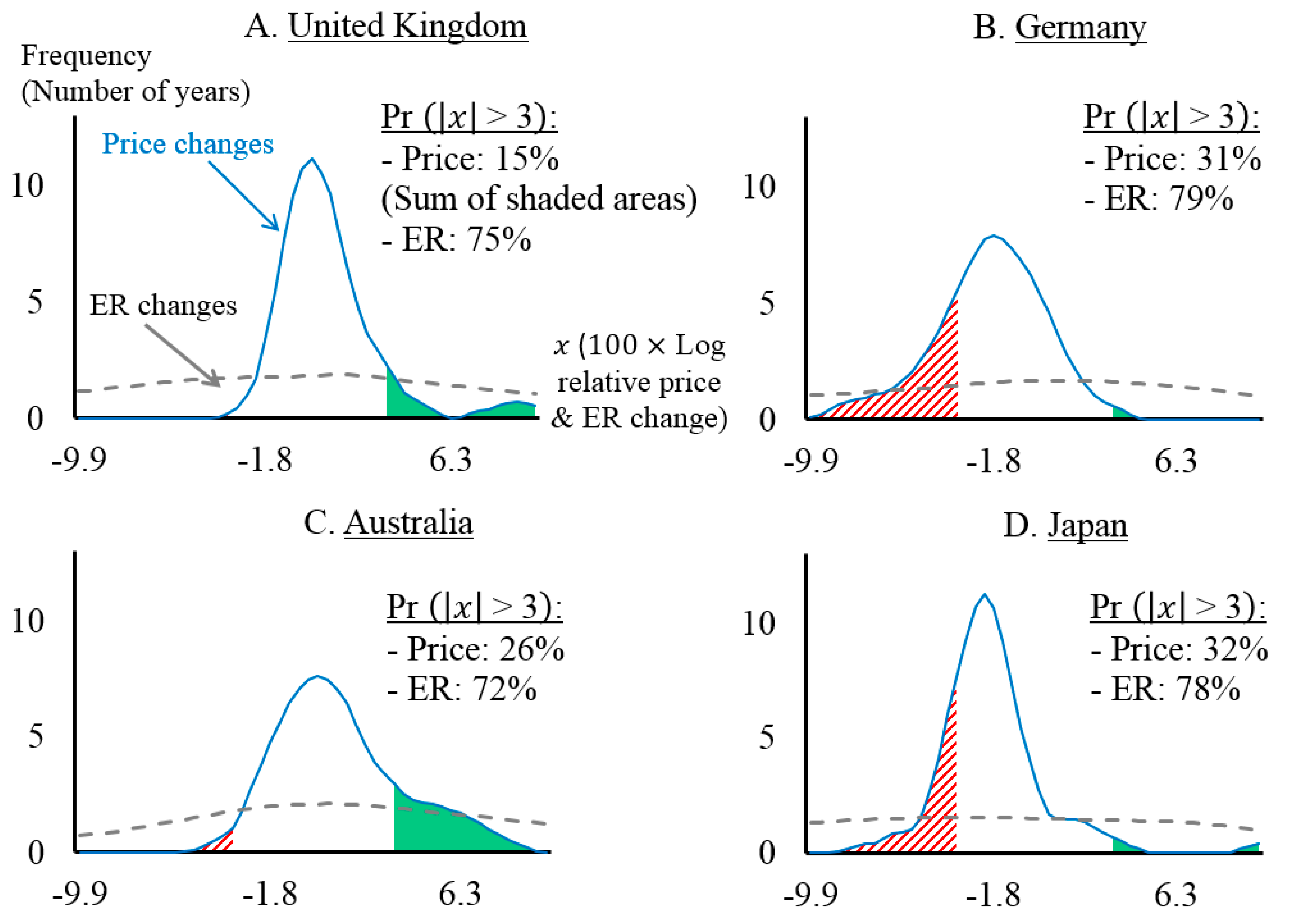
Figure 2.
Multi-resolution plots of USD/AUD time series. Notes: This figure presents the MRA for the full data range from 7th August 2019, to 9:25, 16th September 2019. In each panel, the horizontal axis indicates the corresponding days of the two months.
Figure 2.
Multi-resolution plots of USD/AUD time series. Notes: This figure presents the MRA for the full data range from 7th August 2019, to 9:25, 16th September 2019. In each panel, the horizontal axis indicates the corresponding days of the two months.
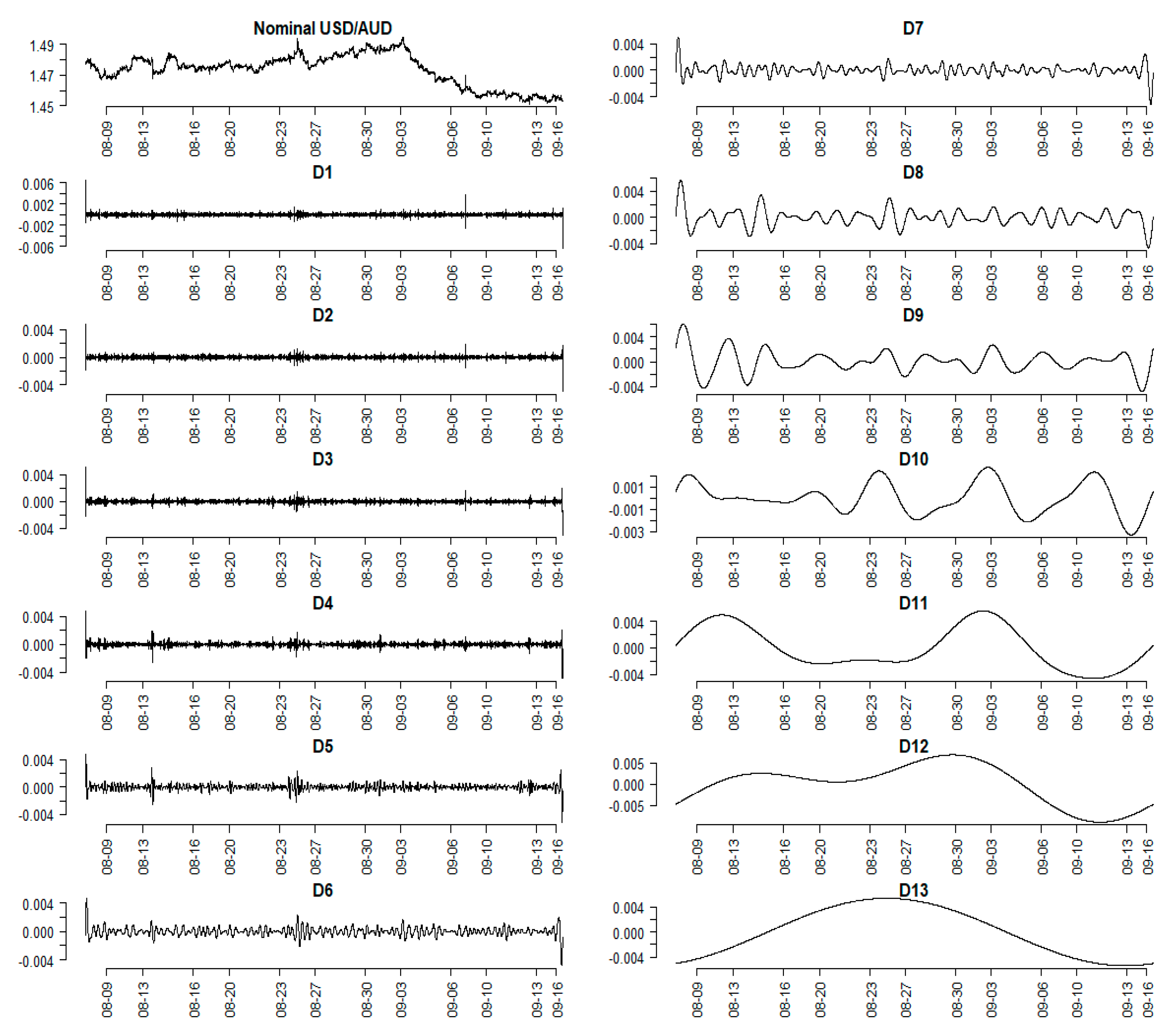
Figure 3.
Auto-correlograms of USD/AUD high-frequency returns and volatilities. Notes: Exchange-rate returns are computed as the log-change of the corresponding five-minute closing spot rates: (t = 1, …, ). Volatilities are defined as the one-day rolling standard deviations of . Source: Authors’ computations.

Figure 4.
Wavelet heat map of five-minute nominal USD/AUD exchange rate. Notes: Horizontal axis ranges from 0 to 8193, the number of five-minute intervals in our sample. The vertical axis indicates the horizons (in five-minute) corresponding to the frequencies at which the underlying time series fluctuates. The power meter is located beneath the graph. The area within the parabolic region indicates the “zone of influence”. The plots were drawn using functions provided in the R package dplR (Bunn 2008). Source: Authors’ computations.


Table 1.
Frequency bands of the first 13 decomposition level.
| Decomposition Level (j) | Frequency Band | Period Band | |
|---|---|---|---|
| In minutes | In days | ||
| (1) | (2) | (3) | (4) |
| 0 (original) | - | - | |
| 1 | 5 to 10 | 0.017 | |
| 2 | 10 to 20 | 0.014 | |
| 3 | 20 to 40 | 0.03 | |
| 4 | 40 to 80 | 0.06 | |
| 5 | 80 to 160 | 0.11 | |
| 6 | 160 to 320 | 0.22 | |
| 7 | 320 to 640 | 0.44 | |
| 8 | 640 to 1280 | 0.89 | |
| 9 | 1280 to 2560 | 1.78 | |
| 10 | 2560 to 5120 | 3.56 | |
| 11 | 5120 to 10,240 | 7.11 | |
| 12 | 10,240 to 20,480 | 14.22 | |
| 13 | 20,480 to 40,960 | 28.44 | |
Source: Authors’ computations.
Table 2.
Summary statistic of five-minute USD/AUD returns and volatilities.
| Mean | Median | Variance | Skewness | Kurtosis | JB | LB(21) | |
| Returns | 0.000001 | 0.00 | 0.00 | 0.72 | 422.12 | 3881823130.38 (0.00) | 9022.43 (0.00) |
| Volatilities | 0.000412 | 0.000393 | 0.00 | 3.70 | 33.17 | 25166002.26 (0.00) | 10405779.70 (0.00) |
Notes: Returns of the USD/AUD exchange rate are computed as the log-change of the corresponding five-minute spot USD/AUD: , where denotes the nominal exchange rate. denotes the number of observations ( five-minute intervals). Volatilities are defined as the one-day rolling standard deviations of . JB and LB denote the Jarque–Bera and the Ljung–Box statistics, respectively. p-values are in parentheses. Source: Authors’ computations.
Table 3.
Long-memory parameter estimates of exchange-rate volatility at different horizons.
| Smooth Level | R/S | aggVar | diffVar | absVal | Higuchi |
|---|---|---|---|---|---|
| Original | 1.101 | 0.966 | 1.620 | 0.980 | 0.966 |
| (0.062) | (0.064) | (0.179) | (0.047) | (0.030) | |
| 1 | 1.146 | 0.966 | 1.618 | 0.980 | 0.966 |
| (0.085) | (0.064) | (0.166) | (0.047) | (0.030) | |
| 2 | 1.056 | 0.966 | 1.747 | 0.980 | 0.966 |
| (0.063) | (0.064) | (0.184) | (0.047) | (0.030) | |
| 3 | 0.994 | 0.966 | 1.663 | 0.980 | 0.966 |
| (0.044) | (0.064) | (0.142) | (0.047) | (0.030) | |
| 4 | 0.988 | 0.967 | 1.833 | 0.980 | 0.966 |
| (0.033) | (0.064) | (0.164) | (0.047) | (0.030) | |
| 5 | 1.005 | 0.968 | 1.965 | 0.981 | 0.966 |
| (0.034) | (0.064) | (0.187) | (0.047) | (0.030) | |
| 6 | 1.008 | 0.972 | 2.174 | 0.984 | 0.966 |
| (0.034) | (0.065) | (0.236) | (0.047) | (0.030) | |
| 7 | 1.003 | 0.978 | 1.756 | 0.986 | 0.965 |
| (0.027) | (0.066) | (0.196) | (0.048) | (0.030) | |
| 8 | 0.990 | 0.988 | 1.803 | 0.992 | 0.965 |
| (0.017) | (0.063) | (0.168) | (0.047) | (0.030) | |
| 9 | 0.993 | 0.997 | 1.932 | 0.999 | 0.966 |
| (0.014) | (0.050) | (0.127) | (0.037) | (0.030) | |
| 10 | 1.000 | 1.003 | 1.669 | 1.007 | 0.966 |
| (0.008) | (0.027) | (0.154) | (0.019) | (0.030) | |
| 11 | 0.999 | 1.001 | 1.364 | 1.005 | 0.966 |
| (0.007) | (0.003) | (0.240) | (0.010) | (0.030) | |
| 12 | 0.999 | 1.002 | 1.468 | 1.005 | 0.966 |
| (0.006) | (0.004) | (0.152) | (0.008) | (0.030) |
Notes: Nomenclatures: (1) R/S: Rescaled range; (2) aggVar: Aggregated variance; (3) diffVar: Differenced variance; (4) AbsVar: Absolute moments; (5) Higuchi: Higuchi’s method. Heteroskedasticity-robust standard errors are in parentheses. Refer to Table 2 for interpretation of the decomposition levels/time-scales. Source: Authors’ computations.
Table 4.
GARCH (1,1) models estimates.
| GARCH | eGARCH | GJRGARCH | fiGARCH | |||||
|---|---|---|---|---|---|---|---|---|
| 0.00 | (0.00) | 0.00 | (0.33) | 0.00 | (0.00) | 0.00 | (0.00) | |
| −0.07 | (0.07) | 0.13 | (0.02) | −0.06 | (0.70) | −0.10 | (0.05) | |
| −0.15 | (0.07) | −0.35 | (0.00) | −0.13 | (0.40) | −0.16 | (0.00) | |
| 0.00 | (0.00) | −2.85 | (0.00) | 0.00 | (1.00) | 0.00 | (0.98) | |
| 0.07 | (0.03) | 0.03 | (0.00) | 0.05 | (0.00) | 0.06 | (0.00) | |
| 0.90 | (0.02) | 0.82 | (0.00) | 0.90 | (0.00) | 0.86 | (0.00) | |
| - | - | 0.32 | (0.00) | 0.05 | (0.00) | 0.85 | (0.00) | |
| Log-likelihood | 54,649.75 | 54,767.86 | 54,228.44 | 54,358.09 | ||||
| Information Criteria | ||||||||
| Akaike | −13.34 | −13.37 | −13.24 | −13.27 | ||||
| Bayes | −13.33 | −13.36 | −13.23 | −13.26 | ||||
| Shibata | −13.34 | −13.37 | −13.24 | −13.27 | ||||
| Hannan–Quinn | −13.34 | −13.37 | −13.23 | −13.27 | ||||
Notes: This table presents estimation results for different GARCH (1,1) specifications described in Section 4. The last row of parameter estimates refers to the asymmetric parameter for the eGARCH and GJRGARCH models, while for the fiGARCH model this refers to the fractional differential parameter . p-Values based on robust standard errors in parentheses.
Table 5.
Number of breakpoints detected using different test statistics.
| Test Type | Test For | GARCH | eGARCH | GJRGARCH | fiGARCH |
|---|---|---|---|---|---|
| Student | Mean changes | 102 | 113 | 93 | 112 |
| Bartlett | Variance changes | 181 | 177 | 191 | 181 |
| GLR | Mean and variance changes | 155 | 154 | 163 | 146 |
| B. Tests in a (possibly unknown) non-Gaussian process | |||||
| MW | Location shifts | 115 | 115 | 112 | 113 |
| M | Scale shifts | 48 | 54 | 44 | 57 |
| KS | Arbitrary changes | 61 | 71 | 53 | 65 |
Notes: The tests listed are applied to residuals from the GARCH models described in Table 5. Nomenclatures: GLR (Generalised Likelihood Ratio), MW (Mann–Whitney), M (Mood) and KS (Kolmogorov–Smirnov). Sources: Authors’ examinations and computations.
© 2020 by the authors. Licensee MDPI, Basel, Switzerland. This article is an open access article distributed under the terms and conditions of the Creative Commons Attribution (CC BY) license (http://creativecommons.org/licenses/by/4.0/).
Share and Cite
MDPI and ACS Style
Vo, L.H.; Vo, D.H. Modelling Australian Dollar Volatility at Multiple Horizons with High-Frequency Data. Risks 2020, 8, 89. https://doi.org/10.3390/risks8030089
AMA Style
Vo LH, Vo DH. Modelling Australian Dollar Volatility at Multiple Horizons with High-Frequency Data. Risks. 2020; 8(3):89. https://doi.org/10.3390/risks8030089
Chicago/Turabian StyleVo, Long Hai, and Duc Hong Vo. 2020. "Modelling Australian Dollar Volatility at Multiple Horizons with High-Frequency Data" Risks 8, no. 3: 89. https://doi.org/10.3390/risks8030089
Note that from the first issue of 2016, this journal uses article numbers instead of page numbers. See further details here.