Figure 1.
Hamiltonian errors of the HMC methods for estimating systemic risk allocations with VaR (left) and RVaR (right) crisis events for the loss distribution (M1). The stepsize and integration time are set to be in Case (I) and in Case (II).
Figure 1.
Hamiltonian errors of the HMC methods for estimating systemic risk allocations with VaR (left) and RVaR (right) crisis events for the loss distribution (M1). The stepsize and integration time are set to be in Case (I) and in Case (II).
Figure 2.
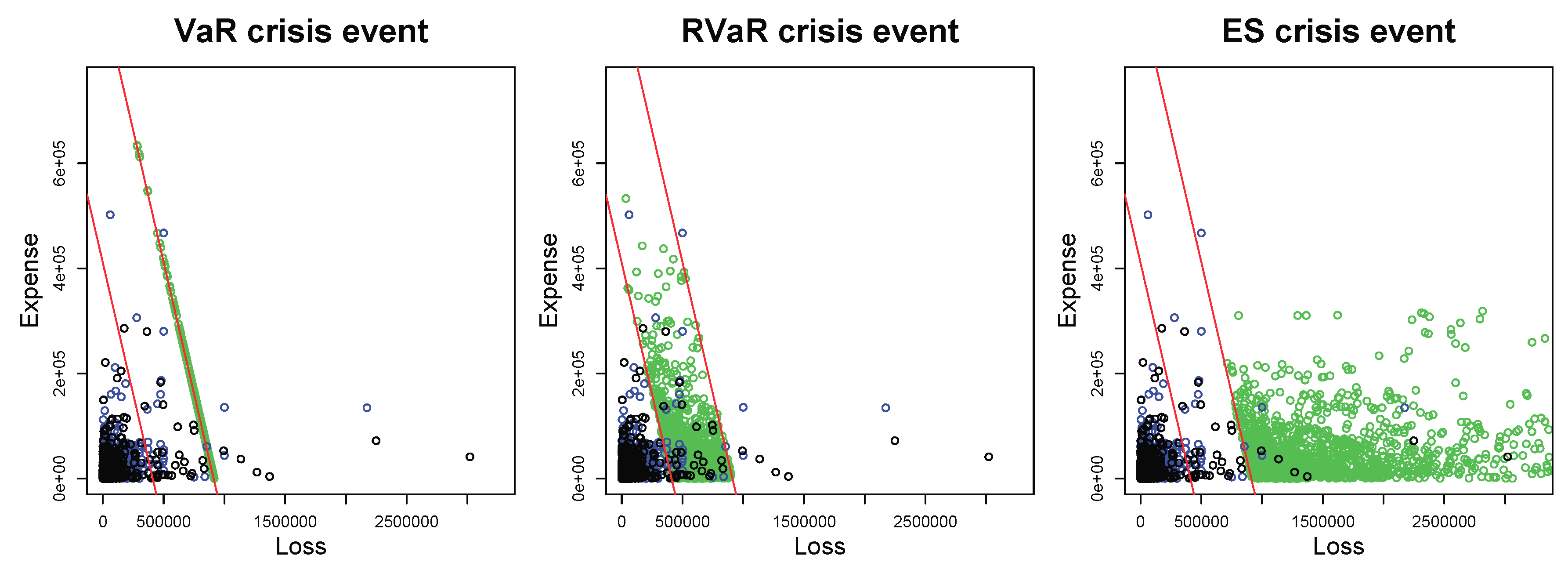
Plots of MCMC samples (green) with VaR (left), RVaR (center), and ES (right) crisis events. All plots include the data and the MC samples with sample size in black and blue dots, respectively. The red lines represent and where and are the MC estimates of and , respectively, for and .
Figure 2.
Plots of MCMC samples (green) with VaR (left), RVaR (center), and ES (right) crisis events. All plots include the data and the MC samples with sample size in black and blue dots, respectively. The red lines represent and where and are the MC estimates of and , respectively, for and .
Figure 3.
Hamiltonian errors of the HMC methods for estimating systemic risk allocations with VaR, RVaR, and ES crisis events for the loss distribution (M3). The stepsize and the integration time are chosen as , and , respectively.
Figure 3.
Hamiltonian errors of the HMC methods for estimating systemic risk allocations with VaR, RVaR, and ES crisis events for the loss distribution (M3). The stepsize and the integration time are chosen as , and , respectively.
Figure 4.
Bias (left), standard error (middle) and time-adjusted mean squared error (right) of the MC, HMC, and GS estimators of risk contribution-type systemic risk allocations under VaR (top), RVaR (middle), and ES (bottom) crisis events. The underlying loss distribution is , where , and for portfolio dimensions . Note that the GS method is applied only to RVaR and ES contributions.
Figure 5.
Bias (left), standard error (middle), and time-adjusted mean squared error (right) of the MC, HMC, and GS estimators of risk contribution-type systemic risk allocations with the underlying loss distribution , where , , and . The crisis event is taken differently, as VaR (top), RVaR (middle) and ES (bottom) for confidence levels , , and . Note that the GS method is applied only to RVaR and ES contributions.
Figure 6.
Bias (left), standard error (middle), and time-adjusted mean squared error (right) of the MC and HMC estimators of risk contribution-type systemic risk allocations under VaR, RVaR, and ES crisis events. The underlying loss distribution is , where , , and . The parameters of the HMC method are taken as determined by Algorithm 4 and . In the labels of the x-axes, each of the five cases and is denoted by HMC.opt, HMC.mm, HMC.md, HMC.dm, and HMC.dd, respectively.
Table 1.
Estimates and standard errors for the MC and HMC estimators of risk contribution, RVaR, VaR, and ES-type systemic risk allocations under (I) the VaR crisis event, and (II) the RVaR crisis event for the loss distribution (M1). The sample size of the MC method is , and that of the HMC method is . The acceptance rate (ACR), stepsize , integration time T, and run time are ACR , , , and run time mins in Case (I), and ACR , , , and run time mins in Case (II).
| | MC | HMC |
|---|
| Estimator | | | | | | |
| (I) GPD + survival Clayton with VaR crisis event: |
| 9.581 | 9.400 | 9.829 | 9.593 | 9.599 | 9.619 |
| Standard error | 0.126 | 0.118 | 0.120 | 0.007 | 0.009 | 0.009 |
| 12.986 | 12.919 | 13.630 | 13.298 | 13.204 | 13.338 |
| Standard error | 0.229 | 0.131 | 0.086 | 0.061 | 0.049 | 0.060 |
| 13.592 | 13.235 | 13.796 | 13.742 | 13.565 | 13.768 |
| Standard error | 0.647 | 0.333 | 0.270 | 0.088 | 0.070 | 0.070 |
| 14.775 | 13.955 | 14.568 | 14.461 | 14.227 | 14.427 |
| Standard error | 0.660 | 0.498 | 0.605 | 0.192 | 0.176 | 0.172 |
| (II) GPD + survival Clayton with RVaR crisis event: |
| 7.873 | 7.780 | 7.816 | 7.812 | 7.802 | 7.780 |
| Standard error | 0.046 | 0.046 | 0.046 | 0.012 | 0.012 | 0.011 |
| 11.790 | 11.908 | 11.680 | 11.686 | 11.696 | 11.646 |
| Standard error | 0.047 | 0.057 | 0.043 | 0.053 | 0.055 | 0.058 |
| 12.207 | 12.382 | 12.087 | 12.102 | 12.053 | 12.044 |
| Standard error | 0.183 | 0.197 | 0.182 | 0.074 | 0.069 | 0.069 |
| 13.079 | 13.102 | 13.059 | 12.859 | 12.791 | 12.713 |
| Standard error | 0.182 | 0.173 | 0.188 | 0.231 | 0.218 | 0.187 |
Table 2.
Estimates and standard errors for the MC and the GS estimators of risk contribution, VaR, RVaR, and ES-type systemic risk allocations under (III) distribution (M1) and the ES crisis event, (IV) distribution (M2), and the RVaR crisis event, and (V) distribution (M2) and ES crisis event. The sample size of the MC method is and that of the GS is . The thinning interval of times T, selection probability and run time are , and run time secs in Case (III), , and run time secs in Case (IV) and , and run time secs in Case (V).
| | MC | GS |
|---|
| Estimator | | | | | | |
| (III) GPD + survival Clayton with ES crisis event: |
| 15.657 | 15.806 | 15.721 | 15.209 | 15.175 | 15.190 |
| Standard error | 0.434 | 0.475 | 0.395 | 0.257 | 0.258 | 0.261 |
| 41.626 | 41.026 | 45.939 | 45.506 | 45.008 | 45.253 |
| Standard error | 1.211 | 1.065 | 1.615 | 1.031 | 1.133 | 1.256 |
| 49.689 | 48.818 | 57.488 | 55.033 | 54.746 | 54.783 |
| Standard error | 4.901 | 4.388 | 4.973 | 8.079 | 5.630 | 3.803 |
| 104.761 | 109.835 | 97.944 | 71.874 | 72.588 | 70.420 |
| Standard error | 23.005 | 27.895 | 17.908 | 4.832 | 4.584 | 4.313 |
| (IV) Multivariate t with RVaR crisis event: |
| 2.456 | 1.934 | 2.476 | 2.394 | 2.060 | 2.435 |
| Bias | 0.019 | −0.097 | 0.038 | −0.043 | 0.029 | −0.002 |
| Standard error | 0.026 | 0.036 | 0.027 | 0.014 | 0.023 | 0.019 |
| 4.670 | 4.998 | 4.893 | 4.602 | 5.188 | 4.748 |
| Standard error | 0.037 | 0.042 | 0.031 | 0.032 | 0.070 | 0.048 |
| 5.217 | 5.397 | 5.240 | 4.878 | 5.717 | 5.092 |
| Standard error | 0.238 | 0.157 | 0.145 | 0.049 | 0.174 | 0.100 |
| 5.929 | 5.977 | 5.946 | 5.446 | 6.517 | 6.063 |
| Standard error | 0.204 | 0.179 | 0.199 | 0.156 | 0.248 | 0.344 |
| (V) Multivariate t with ES crisis event: |
| 3.758 | 3.099 | 3.770 | 3.735 | 3.126 | 3.738 |
| Bias | 0.017 | −0.018 | 0.029 | -0.005 | 0.009 | −0.003 |
| Standard error | 0.055 | 0.072 | 0.060 | 0.031 | 0.027 | 0.030 |
| 8.516 | 8.489 | 9.051 | 8.586 | 8.317 | 8.739 |
| Standard error | 0.089 | 0.167 | 0.161 | 0.144 | 0.156 | 0.158 |
| 9.256 | 9.754 | 10.327 | 9.454 | 9.517 | 9.890 |
| Standard error | 0.517 | 0.680 | 0.698 | 0.248 | 0.293 | 0.327 |
| 11.129 | 12.520 | 12.946 | 11.857 | 12.469 | 12.375 |
| Standard error | 0.595 | 1.321 | 0.826 | 0.785 | 0.948 | 0.835 |
Table 3.
Estimates and standard errors for the MC and HMC estimators of RVaR, VaR, and ES-type systemic risk allocations under the loss distribution (M3) with the (I) VaR crisis event, (II) RVaR crisis event, and (III) ES crisis event. The MC sample size is , and that of the HMC method is . The acceptance rate (ACR), stepsize , integration time T, and run time are ACR , , and run time min in Case (I), ACR , , and run time min in Case (II), ACR , , and run time min in Case (III).
| | MC | HMC |
|---|
| Estimator | | | | |
| (I) VaR crisis event: |
| 842465.497 | 73553.738 | 844819.901 | 71199.334 |
| Standard error | 7994.573 | 7254.567 | 6306.836 | 6306.836 |
| 989245.360 | 443181.466 | 915098.833 | 428249.307 |
| Standard error | 307.858 | 24105.163 | 72.568 | 20482.914 |
| 989765.514 | 500663.072 | 915534.362 | 615801.118 |
| Standard error | 4670.966 | 54576.957 | 669.853 | 96600.963 |
| 990839.359 | 590093.887 | 915767.076 | 761038.843 |
| Standard error | 679.055 | 75024.692 | 47.744 | 31211.908 |
| (II) RVaR crisis event: |
| 528455.729 | 60441.368 | 527612.751 | 60211.561 |
| Standard error | 3978.477 | 2119.461 | 4032.475 | 2995.992 |
| 846956.570 | 349871.745 | 854461.670 | 370931.946 |
| Standard error | 1866.133 | 6285.523 | 2570.997 | 9766.697 |
| 865603.369 | 413767.829 | 871533.550 | 437344.509 |
| Standard error | 5995.341 | 29105.059 | 12780.741 | 21142.135 |
| 882464.968 | 504962.099 | 885406.811 | 529034.580 |
| Standard error | 3061.110 | 17346.207 | 3134.144 | 23617.278 |
| (III) ES crisis event: |
| 8663863.925 | 137671.653 | 2934205.458 | 140035.782 |
| Standard error | 3265049.590 | 10120.557 | 165794.772 | 14601.958 |
| 35238914.131 | 907669.462 | 17432351.450 | 589309.196 |
| Standard error | 2892208.689 | 31983.660 | 443288.649 | 3471.641 |
| 56612082.905 | 1131248.055 | 20578728.307 | 615572.940 |
| Standard error | 1353975.612 | 119460.411 | 1364899.752 | 12691.776 |
| 503537848.192 | 2331984.181 | 25393466.446 | 649486.810 |
| Standard error | 268007317.199 | 468491.127 | 1138243.137 | 7497.200 |


