Bigger Is Not Always Safer: A Critical Analysis of the Subadditivity Assumption for Coherent Risk Measures

Faculty of Business Management and Economics, University of Wuerzburg, Sanderring 2, D-97070 Wuerzburg, Germany
Risks 2019, 7(3), 91; https://doi.org/10.3390/risks7030091
Submission received: 25 June 2019
/
Revised: 16 August 2019
/
Accepted: 20 August 2019
/
Published: 26 August 2019
Abstract
:This paper provides a critical analysis of the subadditivity axiom, which is the key condition for coherent risk measures. Contrary to the subadditivity assumption, bank mergers can create extra risk. We begin with an analysis how a merger affects depositors, junior or senior bank creditors, and bank owners. Next it is shown that bank mergers can result in higher payouts having to be made by the deposit insurance scheme. Finally, we demonstrate that if banks are interconnected via interbank loans, a bank merger could lead to additional contagion risks. We conclude that the subadditivity assumption should be rejected, since a subadditive risk measure, by definition, cannot account for such increased risks.
JEL-Classification:
G21; G32; G341. Introduction
Regulatory bank capital is calculated as a percentage of risk-weighted assets. This is thus an example where risk is measured in monetary units. Conditions for monetary risk measures are given by the theory of so-called coherent risk measures, developed by Artzner et al. (1999). The most important of these conditions is subadditivity, which states that the risk of a portfolio is always less than or equal to the sum of the risks of its parts. Obviously, there is a diversification effect from the merger of two banks A and B, since possible losses of bank A can then be partly or fully offset by gains of bank B. In other words, losses for the merged banking group can never be higher than the sum of the individual losses of bank A and B. Thus, according to this theory, a merger should never lead to an increase in capital requirements1.
Today it is generally accepted not only in academia2, but also by practitioners and regulators, that subadditivity is a necessary requirement for any risk measure. It is therefore considered problematic that value at risk, for many years the industrial standard in financial risk management, is not generally subadditive3. As a consequence of this, the Basel Committee on Banking Supervision (2016), in its new rules for market risk, recently replaced Value at risk by the subadditive risk measure expected shortfall4. It is also believed by the Basel Committee that the lack of subadditivity of value at risk is even more problematic in the area of credit risk and operational risk5. One can therefore expect that the question of subadditivity of a risk measure will be addressed in the context of these other areas of the Basel regulatory framework in the years to come.
But is the subadditivity axiom always an adequate description of how risks are affected by a merger? Consider a merger of two banks A and B, where bank A has a relatively risky portfolio but has taken no loans from other banks, whereas bank B has borrowed heavily in the interbank market. At some point after the merger, a large loss arises in the portfolio that formerly belonged to bank A. That loss could then not only trigger the default of the entire newly merged group, but also of other banks from which bank B has taken loans before the merger. However, had the merger not taken place, then only bank A would default, and bank B would remain solvent as an independent institution and able to repay its interbank loans. Obviously, risk is superadditive and not subadditive in such a case, since new contagion risks are created by the merger.
In addition, if a merger creates a systemically important financial institution (SIFI), certain capital surcharges will be required by the regulator. These SIFI surcharges can be avoided if the merger is reversed and the group breaks itself up again into smaller parts, which is inconsistent with the subadditivity assumption. The risk of a SIFI is higher and not lower than the sum of the risks of its parts6. As another counterexample, the separation of a ‘bad bank’ from a ‘good bank’ is sometimes considered as a mean to reduce risks.
Of course, Artzner et al. (1999) correctly observed that if a given set of assets is held within the same portfolio after a merger, losses might be fully or partly offset by gains from other assets. However, they overlooked that a merger could have the effect of increasing the impact of those losses that remain after such offsetting. This could at least be the case if a merger does not only constitute an internal regrouping. However, an internal reorganization that does not change the legal structure of a bank should have no impact on regulatory capital requirements, provided that the financial position of the bank remains the same. Therefore, in order to analyze the subadditivity assumption, it is indispensable to take into account both the liability structure itself and how it changes through a merger. These changes of the liability structure determine how, e.g., retail depositors and other bank creditors, the deposit insurance scheme, or—as in the above example with interbank lending—other banks are affected by a merger. After all, not the losses as such but the potential adverse effects they might have are the reason that banks are required to hold certain minimum amounts of capital.
It is argued in this paper, mostly in a non-technical way, that, contrary to what is generally believed, the subadditivity assumption could not serve as a universally valid principle in financial risk management. First, it is shown that on an aggregate level, a given amount of losses from loans granted to firms outside the banking sector cannot be reduced by any legal restructuring through bank mergers. A merger only alters the distribution of losses and gains among depositors and other bank creditors on one side and bank owners on the other side. We show that a merger is always beneficial for the creditors of the banks if all creditors are taken together as one group, which then implies corresponding detrimental effects for bank owners. If bank creditors are seen as less sophisticated investors who need more protection than bank owners, this first result might serve as a justification for the subadditivity axiom.
However, this statement is only true if the outcome for all bank creditors together is considered. It does not rule out that some individual bank creditors or holders of certain types of credit such as junior debt will be worse off after a merger. As another counterexample to the subadditivity axiom, we also show that bank mergers can create the necessity that higher total payments have to be made by the deposit insurance scheme. Finally, we investigate in detail under which conditions a merger will reduce or increase the risk of contagion if banks are interconnected via interbank loans. As already demonstrated by the simple example above, a merger could create new contagion risks that would not be present if the banks involved had remained separated.
To summarize, the above examples show that violations of the subadditivity condition are possible in real world examples. Merging two bank portfolios does not always reduce risk, but can also create new risks. This makes the subadditivity assumption problematic as a general principle for risk measures. Nevertheless, there is very little literature with a critical view of the subadditivity assumption. We therefore contribute to the existing literature in providing for the first time an in-depth analysis of the subadditivity assumption.
The few existing discussions about the subadditivity assumption in the literature can be summarized as follows7. Rootzén and Klüppelberg (1999, p. 553), Kou et al. (2013, p. 405) and Krause (2002, pp. 15ff.) point out that contrary to the subadditivity assumption, an institution can reduce risks by splitting off risky business into a separate subsidiary, thereby confining losses to that subsidiary. Dhaene et al. (2003) argue that certain restrictions on dependency structures must be imposed to avoid that the application of subadditive risk measures lead to inconsistencies. Dhaene et al. (2008) show that, if capital requirements are lowered after a merger due to the subadditivity axiom, a larger shortfall arises in those cases where both firms involved in the merger simultaneously generate large losses8. They then introduce a regulator’s condition that balances shortfall risk against the capital costs of the banks, and investigate which risk measure then gives the optimal capital requirement. Recently, Brandtner (2018) has shown that the subadditivity of spectral risk measures implies risk vulnerability. He concludes that if a bank is confronted with increased default risks in its banking book due to an economic downturn, it might at the same time be induced to take more risk in its trading book9.
This paper is organized as follows. The next section gives a brief summary of the concept of coherent risk measures. Section 3 studies the subadditivity axiom in the context of bank mergers. The possible consequences of bank mergers for deposit insurance schemes are analyzed in Section 4. Section 5 is concerned with the relationship of bank mergers and contagion risks. The paper finishes with a short summary and a general discussion on the benefits of diversification.
2. Coherent Risk Measures
The class of coherent risk measures was introduced by Artzner et al. (1997, 1999) who gave four conditions that a risk measure must fulfill in order to be a ‘coherent’ risk measure. They also showed that these conditions are fulfilled for expected shortfall, but not for the traditional value at risk. The most important of these conditions is the subadditivity condition, which is analyzed in detail in this paper. In this section, we recall the conditions for coherent risk measures. The first two of these conditions define what is now called a monetary risk measure. For a monetary risk measure to be a coherent risk measure, the remaining two conditions must also be fulfilled.
A risk measure is defined as a mapping from the set of random variables to the real numbers. Consider a probability space (Ω, F, P) and a linear space Lp of random variables X: Ω → ℝ. In this paper, the values of the random variable X are interpreted as the possible future values in t = 1 of a portfolio10. A special class of risk measures are the so-called monetary risk measures11:
Definition 1.
Monetary Risk Measure
A mapping ρ: Lp → ℝ with ρ(0) = 0 is called a monetary risk measure if the following properties hold:
- (1)
- Monotonicity: If X1 ≥ X2 almost surely, then ρ(X1) ≤ ρ(X2)
- (2)
- Cash invariance or translation invariance12: ρ(X + m) = ρ(X) − m for every m ℝ
The first condition states that if the value of a financial asset will be higher in every state of the world than that of another position, then it is less risky and requires less capital. The second condition states that an additional deposit in cash reduces the risk by exactly the same amount13.
A position is said to be acceptable if it has nonpositive risk ρ(X) ≤ 0. In case of ρ(X) > 0, a further deposit in cash m ≥ ρ(X) is necessary to reduce the risk to or below zero
ρ(X + m) = ρ(X) − m ≤ ρ(X) − ρ(X) = 0
The standard example is an exchange clearing house that guarantees the completion of all transactions concluded by its members and therefore wants to protect itself against the risk that some of its members default. A default might occur in the event of a negative future value X < 0 of a position taken by one of its members (e.g., long or short positions in future contracts). A call for additional funds arises in such a situation, which the exchange member might not be able to satisfy. An ex-ante additional cash deposit or margin payment is therefore required by the exchange. The value of the position then increases in every possible future state, thereby reducing the probability of negative future values. The size of the margin payment is determined by the risk measure ρ(X). If ρ(X) > 0 for a given position X, the position is not acceptable and the exchange will require a further margin payment m ≥ ρ(X) so that the resulting risk ρ(X + m) = ρ(X) − m is nonpositive.
In the context of regulatory bank capital requirements, it has to be noted that capital requirements do not refer to the amount of cash the bank holds on the assets sides of its balance sheet. Instead, regulatory capital requires a minimum amount of equity on the liabilities side of the balance sheet. Here, the random variable X denotes the nonnegative14 future value of the bank’s assets and ρ(X) the corresponding capital requirement. There are two possibilities for a bank in case of a capital shortfall: the bank could either alter the probability distribution of X by selling assets or by replacing them with less risky assets15. The objective is to reduce the risk ρ(X) so that it is no longer greater than the existing amount of capital. A second possibility is that additional capital is paid in to close the capital gap. The additional capital is then either invested into assets with zero risk weight or used to repay debt.
The theory of coherent risk measures is based on the assumption that a reasonable risk measure should satisfy two additional conditions16:
Definition 2.
Coherent Risk Measure
A monetary risk measure is a coherent risk measure if the following properties hold:
- (1)
- Positive homogeneity: ρ(λX) = λ ρ(X) for all XLp and λℝ≥0.
- (2)
- Subadditivity: ρ(X1 + X2) ≤ ρ(X1) + ρ(X2) for all X1, X2Lp
The positive homogeneity condition states that the risk of a position is proportional to its size. If, for example, the number of future contracts is doubled or trebled, the margin requirement doubles or triples as well. For λ = 0, homogeneity also implies ρ(0) = 0 (normalization), which had to be explicitly assumed above in the definition of monetary risk measures.
The assumption of positive homogeneity has been criticized because of liquidity risks for large portfolios. Whereas a smaller portfolio might be liquidated at given prices, the liquidation of a large portfolio could have an impact on the market prices. Increasing the size of a portfolio by a factor λ > 1 could then increase its risk by more than the factor λ, i.e., ρ(λX) > λρ(X). This also implies a violation of the subadditivity assumption in the case of λ = 2 with X1 = X2. One approach to incorporate liquidity risks is to alter the distribution assumptions of the random variables by adjusting the payoffs to liquidity risks and maintaining the axioms of coherent risk measures, see (Acerbi and Scandolo 2008; Artzner et al. 1999, p. 209, Remark 2.8).
The subadditivity assumption is meant to capture the idea of diversification. As an illustration, consider again the example of an exchange clearing house and assume that two exchange members merge their respective portfolios. This is advantageous from the perspective of the clearing house, since a negative value of the position of one exchange member might then be offset by a positive value of a position of another exchange member. The merger has the effect that both exchange members are liable for every potential loss. As a result, a call for additional funds will not arise in some cases where it would arise had no merger occurred. This might induce the clearing house to reduce the margin requirement compared to the case of two separated portfolios. At least, a merger should never lead to an increase of margin requirements.
Mathematically, the amount of a potential call for additional funds in case of a negative position value X is given by −min(X + m, 0) ≥ 0 if a margin payment m was made. In case of a merger, the following inequality obviously holds
−min(X1 + m1 + X2 + m2, 0) ≤ −min(X1 + m1, 0) − min(X2 + m2, 0)
Inequality (2) states that in every future state of the world, a potential call for additional funds for a merged portfolio would be lower or equal than the sum of such calls for two separate portfolios. This confirms the subadditivity assumption, which states that the margin requirement for a merged portfolio should never be larger than the sum of the margin requirements for two separate portfolios17.
3. Subadditivity and Bank Mergers
In the last chapter, it was shown that subadditivity is a rational assumption for margin requirements. It is now asked whether the subadditivity assumption could also be justified in the context of regulatory bank capital requirements.
As an illustration, consider the consolidated balance sheet of all banks in an economy where all internal positions where the counterparty is also a bank are netted out in the process of consolidation. Now assume that some loans granted to non-banks are not fully paid back, thereby causing losses to the financial system. Left and right sides of the consolidated balance sheet would then shrink by exactly the same amount. These losses are first absorbed by the capital of the institution that has granted those loans. If that capital is completely wiped out, the bank will not be able to fulfill all her liabilities and the creditors of that bank bear the remaining losses. The capital of other banks would not be liable for these losses. One could speak of firewalls that exists between different banks18.
Such firewalls are eliminated if a merger between two different bank occurs. After a merger, the combined capital of both banks involved is liable for potential losses from asset write-downs. It is assumed here that no change of any kind in the business policy of the banks involved in a merger takes place. Any potential future cost savings etc. from a merger are also neglected. The size of these write-downs is then independent from a merger as a purely legal act, since these losses depend only on the ability of non-financial corporations in the real economy to repay their loans. Therefore, the asset side and the total size of the consolidated balance sheet of all banks would not change due to a merger. A merger only has an effect on the structure (but not on the size) of the liability side of that balance sheet, as losses are allocated differently between owners and creditors of the two banks involved in a merger.
For the purpose of formal analysis in a one-period model, denote by X the future nonnegative asset value in t = 1 and by D the face value of a banks’ total debt. Creditors of the bank receive either the full amount D or, in case of a default, a payment equal to the value X of the banks’ assets19, whereas bank owners receive the remaining residual
Payoff to bank creditors: min(X, D)
Payoff to bank owners: X − min(X, D) = max(0, X − D)
Now assume the case of two banks. One could then compare the combined payoff in t = 1 to the creditors of both banks depending on whether a merger of the two banks has occurred in t = 0 or not. The same can be done for the payoff to bank owners. The following inequalities hold
min(X1, D1) + min(X2, D2) ≤ min(X1 + X2, D1 + D2)
max(0, X1 − D1) + max(0, X2 − D2) ≥ max(0, X1 + X2 − D1 − D2)
Inequality (3) shows that for every possible future realization of asset values, the combined payoff to the creditors of both banks is higher following a merger than it would be without a merger. Inequality (4) shows that the reverse is true for the owners of the bank.
A merger is therefore always beneficial to the creditors of the banks and disadvantageous for its owners. This result may be seen as a confirmation for the subadditivity assumption if the regulator adopts the view that bank creditors, and bank depositors in particular, need more protection than bank owners, who may be viewed as more sophisticated investors. According to this line of reasoning, better protection of bank creditors due to a merger could justify reduced capital requirements for the merged institution. The above analysis would then make explicit the so far hidden assumptions on which the subadditivity axiom implicitly relies.
However, owners, on the other hand, would always prefer that both banks stay separated (inequality (4)). As an illustration, note that it is advantageous for a holding company of a large financial group to conduct its many businesses through a number of legally independent subsidiaries with limited liability. Merging those subsidiaries would create the risk that losses from one line of business—e.g., from operations in a certain country—could also endanger the business of other subsidiaries. Such a merger would only benefit the creditors of the subsidiaries, since it would increase the amount of assets liable for their claims. However, from the viewpoint of the holding company as owner of the subsidiaries, subadditivity does not apply, since merging subsidiaries would create additional risks for the firm20.
Furthermore, the above inequalities (3) and (4) are no longer true if other types of debt such as hybrid capital or junior debt are also taken into consideration. To see why a bank merger could create extra risk for junior debtholders, consider a merger between a bank A with junior and senior debt and a second bank B with only senior debt. At some point after the merger, borrowers who have lent money from bank B get into trouble and a massive write-down of the respective loans is necessary. These asset write-downs could then not only wipe out the entire capital of the newly merged banking group, but could also lead to losses for the junior debtholders. However, had a merger not occurred and had the two banks stayed separated, junior debtholders of bank A would have been better off since they are then not affected by the asset write-downs of bank B. This example is of some practical relevance since junior bonds are occasionally sold to supposedly risk-averse retail investors21.
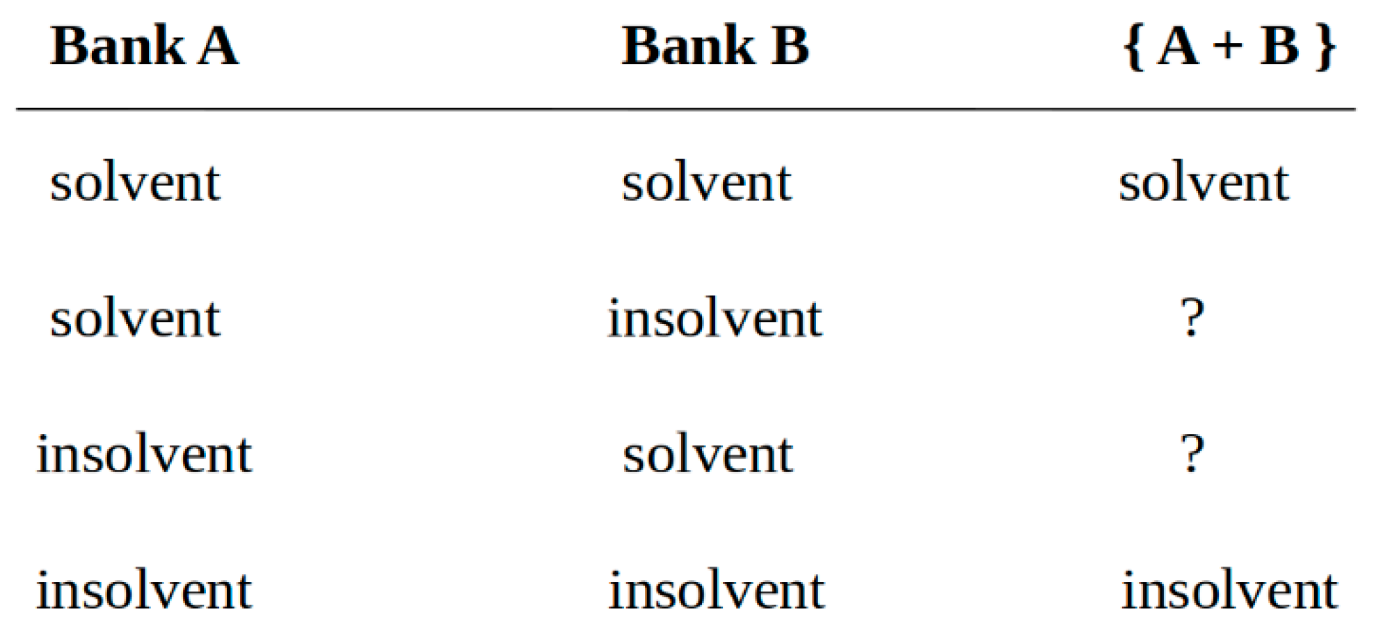
Even if differences between junior and senior debt are put aside, and assuming that there are no differences in the ranking order of debt issued by banks, it should be noted that the above result is only valid if the combined payoff to all creditors of both banks is considered. It could be that the merger has the effect that the payoff in fact decreases for some creditors22, if the payoff to other creditors rises even more. For further analysis, it is useful to distinguish different cases as shown in Figure 1.
In the first two columns of Figure 1, the stand-alone case is considered and four cases are distinguished according to whether bank A and/or bank B will be solvent or insolvent in t = 1 if no merger has occurred in t = 0. In the third column, it is stated whether a merged firm would be solvent or not in t = 1.
If at t = 1 both banks are solvent in the stand-alone case (first row), then of course there would be no insolvency in case of a merger. In the second and third row, an asymmetric shock unexpectedly triggers the default of one of the two banks in the stand-alone case. For example, think of two banks that specialize in different business areas or operate in different geographic areas. The solvency of a merged group then depends on whether the asymmetric shock is of medium or large size23. If it is of medium size, the equity of both banks together is large enough to absorb the losses24. A default is thus avoided by a merger. If, e.g., bank B is affected by a medium sized shock, a merger would end up being advantageous for owners and creditors of bank B at the expense of the owners of bank A, who then have to bear additional losses but will not be completely wiped out, whereas nothing changes for the creditors of bank A.
If the asymmetric shock by which bank B is affected is instead sufficiently large, even the combined capital of both banks A and B would not be able to absorb the corresponding losses. As a result, the merged group would also default and owners of both banks would be completely wiped out. However, in this case, the merger would also be detrimental for creditors of bank A, whereas creditors of bank B would benefit from a higher insolvency quota. In addition, it follows from inequality (3) above that losses to the creditors of bank A are smaller than the gains to the creditors of bank B, since all creditors combined are always better off following a merger.
Finally, the case where both banks are insolvent in t = 1 has to be dealt with (last row). All bank owners will then be completely wiped out regardless of whether a merger has taken place or not. Creditors will receive payments according to an insolvency quota that will be the same for all creditors in case of a merger. Compared to the stand-alone case, this insolvency quota will be higher for the creditors of one bank and lower for the creditors of the other bank, depending on the remaining values of the assets and the existing debt.
For a general analysis, define the insolvency quota q as
q = min(1, X/D)
As above, X denotes the asset value at t = 1 and D denotes the nominal amount of debt. The case of no default is also included if25 q = 1. If two banks with insolvency quotas q1 and q2 merge, the insolvency quota of the merged entity is denoted by qm. A bank creditor receives a lower payoff as a result of a merger if qm < qi. The following general result states that qm is always in between the two insolvency quotas q1 and q2 in the stand-alone case:
Lemma 1.
Let q1 = min(1, X1/D1) and q2 = min(1, X2/D2) denote the insolvency quotas for bank A and bank B and qm = min[1, (X1 + X2)/(D1 + D2)] the insolvency quota of the merged group. Assume, without loss of generality, q1 ≤ q2. Then for every possible realization of the asset values X:
q1 ≤ qm ≤ q2
Proof.
Appendix A. □
The result shows that the quota creditors receive after a merger is always higher (or equal) for the creditors of one bank and lower (or equal) for creditors of the other bank than it would be without a merger.
4. Subadditivity and Deposit Insurance
In most countries, bank deposits are protected by certain guarantee schemes with the aim of enhancing depositor confidence and avoiding bank runs. At the same time, such guarantees make funding cheaper for banks, since interest rates on guaranteed deposits do not reflect the default risk of the bank. This induces an incentive for banks for excessive indebtedness26, which is then counteracted by the regulator by setting certain minimum capital ratios. These regulatory capital requirements reduce the probability that the deposit insurance has to be actually invoked.
Therefore, an important objective of the regulator is to avoid any losses to the insurance scheme. In this section, we analyze whether risks for the insurance scheme are always reduced by a merger, as the subadditivity assumption would predict. Consider at first the hypothetical case where all deposits and other loans to the bank are insured in full27. As has been shown by inequality (3) above, the payoff to all bank creditors as a group increases with a merger for any future realization of the asset values. Though some individual creditors might suffer greater losses than without a merger, this is always more than compensated by smaller losses to other creditors. It follows that a merger is always beneficial to the insurance scheme under the assumption of full insurance, since only the overall loss compensation that must be paid out is then relevant to the scheme.
However, a different result is obtained if not all liabilities of the bank are covered by the insurance scheme. Consider as a simple example a merger between a commercial bank and an investment bank. Only the retail depositors of the commercial bank are covered by the insurance scheme, but not institutional investors who have lent to the investment bank. Assume that, after a merger, major losses occur in the investment banking part that lead to a default of the newly merged group. Depositors of the formerly independent commercial bank must then be compensated by the insurance scheme. Such compensation could have been avoided had a merger not taken place. In this case, and contrary to the assumptions that underlie the subadditivity condition, additional risks to the deposit insurance scheme arise through a merger.
In addition, bank deposits are usually only insured up to a certain amount. In case of a bank default, depositors will be only compensated up to this amount, and to that extent their claims are assigned to the deposit insurance scheme28. The scheme then files these claims with the insolvency administrator. The portion of depositors’ claims that exceed the guaranteed level have to be filed with the administrator by the depositors themselves. These excess claims and the claims filed by the insurance scheme have equal ranking (pari passu) in most jurisdictions29. This is in particular the case in the EU30 or in the US31. Under this legal framework, it can be shown that a merger may be, in certain cases, disadvantageous for the deposit insurance scheme even if banks fund themselves exclusively through retail deposits.
As a numerical example, assume that bank A has total deposits of 200 monetary units. Of these, 20 units are covered by deposit insurance. In t = 1, the value of bank A assets is only 40 units. Therefore, the bank defaults and the deposit insurance scheme has to pay 20 units to the depositors of the bank. An assigned claim in the same amount is then filed by the scheme with the insolvency administrator. In addition, depositors file their excess claims in the amount of 180 units with the administrator. With total debt of 200 units and assets worth 40 units, the insolvency quota is 20%. The scheme can therefore recover 20% of the amount paid to the depositors through the insolvency procedure. This results in a net loss of 16 units to the scheme.
Now consider a merger with a second bank B with total deposits of 100 units, of which 90 units are covered by deposit insurance. Bank B assets are worth 140 units in t = 1. Since bank B is solvent in t = 1, no payments by the scheme are necessary in the stand-alone case. In case of a merger of the two banks, total debt of the combined group would be 300 units, and assets combined are worth 180 units. This results in an insolvency quota of 60%. The payout by the deposit insurance scheme is 20 + 90 = 110 units in case of a merger, of which the scheme can recover 60% through insolvency proceedings. The net loss to the scheme is now 44 units instead of only 16 units in the stand-alone case. Figure 2 provides a graphical illustration. Note that depositors of bank A benefit in case of a merger from an increase of the insolvency quota for their excess claims from 20% to 60%. These gains correspond to losses to the owners of bank A and to the insurance scheme.
To conclude, the following lemma provides general conditions under which a merger is detrimental to the deposit insurance scheme.
Lemma 2.
Denote the insured amount of deposits at bank A and B with S1 and S2 respectively. The default of the merged entity implies qm < 1. Assume, without loss of generality, q1 < q2 and that at least bank A would default in the stand-alone case, or q1 < 1.
Then, if q2 < 1, the condition that the deposit insurance scheme is worse off after a merger is given by
S1/D1 < S2/D2
If q2 = 1, the condition is given by
S1/D1 < S2 (D1 + D2 − X1 − X2)/(X2D1 − D2X1)
Proof.
Appendix B. □
There are two cases. If both banks would default in the stand alone case (q2 < 1), a merger is detrimental for the deposit insurance scheme if bank A (whose creditors would receive a higher quota after a merger) has a lower proportion of insured deposits Si as part of all deposits Di as compared to bank B. It is intuitively clear that if the proportion of insured deposits is exactly the same at both banks, the deposit insurance scheme is indifferent to a merger, since it would then receive the same proportion of assets as a result of the insolvency procedures, regardless of whether a merger has taken place or not. If the proportion of insured deposits differs, a merger primarily benefits the uninsured excess claims against bank A. In the second case, where only bank A, but not bank B would default in the stand-alone case (q2 = 1), a more complicated condition arises.
5. Subadditivity and Contagion Risk
Banks are often connected with each other through interbank lending. The default of a bank may then cause the default of other banks which have lent to it. If these other banks have also borrowed in the interbank market, even more banks could default in a second round, and so on. A chain of bank failures would then be triggered. In the context of this study, we are interested in whether such contagion effects are increased or mitigated by a bank merger.
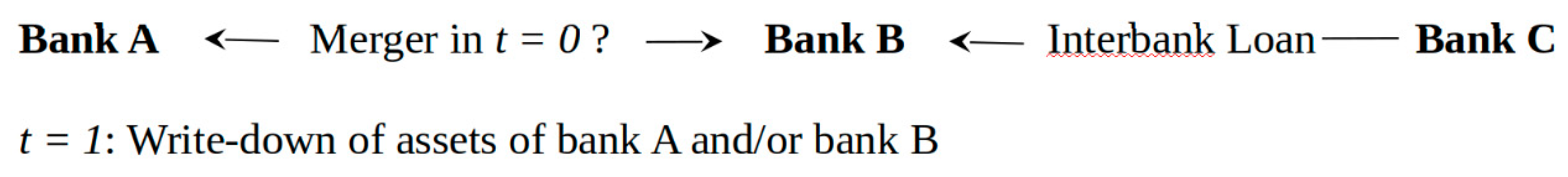
Consider again two banks, A and B, where bank B has now taken a loan from a third bank C (Figure 3). In t = 1, a write-down of assets might be necessary, which could trigger the default of one or both banks. We want to compare the consequences of such a write-down depending on whether a merger of bank A and B has or has not occurred in t = 0. Again, it is helpful to distinguish between different cases as given by Figure 1 in Section 3. In the first case, there is no bank default and all interbank loans are repaid in full, regardless of whether a merger has taken place or not. In the second case, bank B but not bank A would default in t = 1 in the stand-alone case (second row of Figure 1). Contagion risks are then mitigated as a consequence of a merger: A merger of the two banks would either have the effect that the merged bank does not default on the interbank loan (if losses are of medium size) or bank C would at least receive a higher fraction of its claim against bank B as a result of insolvency proceedings.
By contrast, a contradiction to the subadditivity axiom could arise in the case given by the third row of Figure 1, where bank A instead of bank B would default in the stand-alone case. Without a merger, the interbank loan bank C has given to bank B would then be repaid in full. This may no longer be the case in the event of a merger, since the write-down in the loan portfolio that belonged to bank A could be so large that the entire newly merged group defaults on its liabilities. Such increased contagion risks are never accounted for by a subadditive risk measure, since such a risk measure would always consider the merged group as less or at least equally risky.
Finally, the case where write-downs at both banks A and B would trigger their default in the stand-alone case has to be considered (fourth row of Figure 1 in Section 3). If both banks would have merged before these write-downs, the emerging banking group would also always default. It follows directly from the results in Section 3 that a merger could result in a higher or lower insolvency quota that bank C will receive on its claim against bank B.
In summary, contagion risks can both decrease or increase as a result of a merger. A medium-size loss may be absorbed by the combined capital of the two banks, whereas a very high loss could lead to a default on the interbank loan that could have been prevented if the banks had remained separate entities. The likelihood of these different scenarios is ultimately an empirical question32. However, the subadditivity axiom is supposed to be a self-evident assumption that is generally true and not dependent on whether certain conditions are actually met in reality.
So far, it has only been considered whether or not contagion risks are more pronounced after a merger. For bank creditors, the recovery rate in the event of an actual default is also of importance. We now examine as an extension to the analysis in Section 3 how a merger affects the payoffs to external creditors and owners. The term ‘external creditors’ excludes bank C (which is a creditor of bank B) and comprises only non-bank creditors of banks A, B, and C. Therefore, in order to determine the payments to external creditors, the overall amount bank B pays to its creditors must be reduced by the payment it makes to bank C. It must also be considered that payments from B to bank C increase the amount available for distribution at bank C. In addition to the notations in previous sections, the amount of bank C’s assets other than the loan given to bank B is denoted by X3 and the nominal value of the loan that bank C has given to bank B is denoted by L with L ≤ D2. First, the case where no merger has occurred is considered:
Payoffs to external bank creditors:
Payoff to external creditors of bank A:
D1q1 = min(X1, D1)
Payoff to external creditors of bank B:
(D2 − L) q2 = (1 − L/D2) min(X2, D2)
Payoff to external creditors of bank C:
min(X3 + L q2, D3)
Payoffs to bank owners:
Payoff to owners of bank A:
X1 − D1 q1 = max(X1 − D1, 0)
Payoff to owners of bank B:
X2 − D2 q2 = max(X2 − D2, 0)
Payoff to owners of bank C:
max(X3 + L q2 − D3, 0)
It can be easily verified that the sum of all payoffs to all owners and external creditors together always equals X1 + X2 + X3, which is the sum of all existing assets excluding interbank loans, which are netted out. The above formulas therefore show how payoffs from loans to borrowers outside the financial system are divided into payoffs to external owners and creditors of the banks.
These division rules change in case of a merger:
Payoffs to external bank creditors:
Payoff to external creditors of merged banks A and B:
(D1 + D2 − L) qm = [1 − L/(D1 + D2)] min(X1 + X2, D1 + D2)
Payoff to external creditors of bank C:
min(X3 + L qm, D3)
Payoffs to bank owners:
Payoff to owners of merged banks A and B:
X1 + X2 − (D1 + D2) qm = max(X1 + X2 − D1 − D2, 0)
Payoff to owners of bank C:
Again, payoffs to all owners and external creditors combined always sum up to X1 + X2 + X3.
max(X3 + L qm − D3, 0)
We now focus on whether all external creditors combined receive a higher or lower payoff as a result of a merger. It is useful to distinguish two cases according to whether the recovery rate for creditors of bank B is higher (qm > q2, second or fourth row of Figure 1) or lower (qm < q2, third or fourth row of Figure 1) as a result of a merger of banks A and B. The payment bank C receives on the interbank loan will then be also either higher or lower in these cases. If payments to creditors of bank B increase as a result of a merger, then part of this increase will be absorbed by bank C, but external creditors of bank C do not necessarily benefit from this increase. If for example X3 > D3, assets of bank C are large enough that it would never default, irrespective of the quota it receives on the interbank loan. Since it follows from lemma 1 that creditors of bank A will receive a lower or equal quota if the quota for creditors of bank B increases due to a merger, external creditors of bank B (other than bank C) are the only creditors who would benefit from a merger. Assume further that bank B has only very few external creditors and is almost exclusively funded by bank C, i.e., L ≈ D2. In this extreme case, and contrary to our result in Section 3, all external creditors combined could receive a lower payoff after a merger has taken place33.
Now assume the other case where the recovery rate for creditors of bank B is lower as a result of a merger of banks A and B (qm < q2). According to the results of Section 3, creditors of bank A would then, conversely, receive a higher recovery rate. It can be concluded that all external creditors combined receive a higher payoff, since all creditors of bank A are external creditors. Note that, for the constellation given in Figure 3, our result from Section 3 that external creditors as a whole always get a higher payoff as a result of a merger can only be generalized to the case with interbank loans if qm < q2, i.e., if contagion risks are more(!) pronounced after a merger.
It is difficult to make general statements for more complex networks. Consider a complex network of interconnected banks linked with each other through interbank loans. In t = 1, an external shock requires certain write-downs in the loan portfolios of the banks. After accounting for network effects through contagion, these write-downs result in a number n of bank defaults. Assume now that in t = 0, before the shock occurs, a merger of two banks has taken place. Assume further that, all else equal, that the same external shock now results in a number n* > n of bank defaults in t = 1. Since n* > n, a greater number of bank owners is wiped out. At the same time, the value in t = 1 of the aggregated loan portfolio of all banks in the network does not depend on whether a merger has occurred in t = 0 or not. This value only depends on the size of the external shock. Since the value of all assets available for distribution remains the same, any additional losses for bank owners must correspond to higher gains for external creditors. However, from this it cannot be concluded that external creditors as a group always receive a higher payoff if a merger results in a higher number of bank defaults. It must also be taken into account that n* > n does not rule out that in an arbitrarily complex network, recovery rates can be higher for certain other interbank loans, and this could benefit some of those bank owners who are not wiped out. No general statement can therefore be made on whether the payoff to all external creditors combined increases or decreases if a merger of two banks leads to a higher number of bank defaults.
6. Summary and Discussion
The conventional view is that the subadditivity axiom is a necessary part of a consistent or ‘coherent’ theory of risk measurement in order to ensure that diversification effects are properly accounted for. The concept of coherent risk measures is intended as a general theory applicable to the measurement of the risk of not only individual credit departments and trading desks but also of large financial groups which are made up of many legally independent entities. In this paper, it was shown that—contrary to what is stated by the subadditivity assumption—mergers can create extra risk. A risk measure that correctly reflects these extra risks can therefore not be generally subadditive. Put differently, a subadditive risk measure, by definition, cannot account for such increased risks. Subadditivity of risks does not always apply in reality.
The objective of this paper and the main findings can be summarized as follows:
- According to the subadditivity assumption of Artzner et al. (1999), a merger does not create additional risk. In order to check this assertion, a merger of two bank portfolios with given payoffs has been considered. It was assumed that the merger only alters the legal structure, but not the payoffs of the two bank portfolios.
- A merger then alters the distribution of payoffs between creditors and owners. If taken as one group, bank creditors always receive a higher payoff after a merger, and the reverse is true for bank owners. However, this does not rule out that some individual creditors or holders of certain types of debt (e.g., junior debt) can be worse off after a merger.
- If a deposit insurance scheme exists, a merger can also create a higher risk for such a scheme. It is possible that the scheme must make a higher payout than it would be the case without a merger.
- If banks are linked via interbank loans, a merger could also lead to higher contagion risks. In addition, the result that a merger always increases the payoffs for all bank creditors combined cannot be generalized to arbitrarily complex networks of interbank loans.
Possible consequences for the future direction of the theory of financial risk measures should be briefly discussed. One suggestion could be to simply replace the subadditivity assumption by alternative concepts to model diversification such as quasi-convexity or convexity34. Generally, a more diversified bank portfolio increases the market value of bank debt, while bank owners would prefer a more risky policy35. Obviously, this is analogous to our result in Section 3 that a merger is always beneficial for bank creditors. A risk measure that encourages diversification should therefore be used if the objective is to prevent losses to bank creditors from a lower market value of bank debt36.
However, in our view, the problem lies deeper because the underlying assumption that more diversification of individual bank portfolios is always beneficial is questionable. A more diversified bank portfolio could increase the default probability of a bank37. Diversification is often characterized as not putting all eggs into one basket. If a bank diversifies its investments among many different projects, losses will be lower (since it will lose only a few baskets) in most cases, but the probability that a loss arises will be higher (since there are many baskets). However, for a bank with very little equity, even a small loss might be sufficient to cause a default. Diversification would then increase the default probability of the bank. Consider as an example two stochastically independent investment projects that both provide a gain of 5% with probability of 99% and a loss of 25% with 1% probability. A bank with, e.g., 8% capital that invests in only one of these projects would then have a default probability of 1%. However, if the bank instead diversifies and invests in equal parts in both projects, the default probability would almost double to 1 − 0.992 = 1.99%.
This is not a contradiction of the fact that diversification raises the market value of debt, since market value also depends on the amount of losses if a default actually occurs. However, a regulator will often be primarily concerned about the default probability of a bank independently of the eventual recovery rate for bank creditors. This will in particular be the case for systemically important institutions. Note that if it is only of interest whether or not a bank will default, then value at risk is the appropriate risk measure. Value at risk is defined as the loss that will not be exceeded with a given probability 1 − α. Therefore, a bank whose capital is determined as value at risk with confidence level 1 − α has a default probability not greater than38 α. That value at risk is not subadditive and does not always account for diversification corresponds to the fact that more diversification of a banks’ portfolio could increase the default probability of the bank39.
To summarize, the main problem is not how the subadditivity axiom translates diversification into a formal model. Rather, in our opinion, the underlying assumption that more diversification of individual bank portfolios is always and without exception beneficial should be revised.
Funding
This publication was funded by the German Research Foundation (DFG) and the University of Wuerzburg in the funding program Open Access Publishing.
Acknowledgments
I would like to thank participants of the 36th International Symposium on Money, Banking and Finance, Besancon, 12–14 June 2019 for helpful comments.
Conflicts of Interest
The author declares no conflict of interest.
Appendix A
Proof of Lemma 1
(a) Proof of q1 ≤ q2 => q1 ≤ qm
First assume that X1/D1 ≤ X2/D2, then:
<=> D2X1 ≤ D1X2
<=> D1X1 + D2X1 ≤ D1X1 + D1X2
<=> X1/D1 ≤ (X1 + X2)/(D1 + D2)
=> q1 = min(1, X1/D1) ≤ qm = min[1, (X1 + X2)/(D1 + D2)]
Now assume that X1/D1 > X2/D2. Because of q1 ≤ q2 this implies X1/D1 > X2/D2 > 1 and therefore X1 + X2 > D1 + D2. It follows that q1 = qm = 1.
(b) Proof of q1 ≤ q2 => qm ≤ q2
First assume that X1/D1 ≤ X2/D2, then:
<=> D2X1 ≤ D1X2
<=> D2X2 + D2X1 ≤ D2X2 + D1X2
<=> (X1 + X2)/(D1 + D2) ≤ X2/D2
=> qm = min[1, (X1 + X2)/(D1 + D2)] ≤ q2 = min(1, X2/D2)
Now assume that X1/D1 > X2/D2. Because of q1 ≤ q2 this implies X1/D1 > X2/D2 > 1 and therefore X1 + X2 > D1 + D2. It follows that q1 = qm = 1. □
Appendix B
Proof of Lemma 2
Loss of the deposit insurance scheme in the stand-alone case:
S1 − S1 q1 + S2 − S2 q2
Loss of the deposit insurance scheme in case of a merger:
S1 + S2 − (S1 + S2) qm
The deposit insurance scheme is worse off after a merger if:
S1 + S2 − (S1 + S2) qm > S1 − S1 q1 + S2 − S2 q2
<=> S1 (q1 − qm) > S2 (qm − q2)
It follows from q1 < q2 together with Lemma 1 that q1 − qm < 0 and qm − q2 < 0, therefore:
q1 < 1 and qm < 1 implies q1 = X1/D1 and qm = (X1 + X2)/(D1 + D2). Therefore:
S1 < S2 (q2 − qm)/(qm − q1)
S1 < S2 [q2 − (X1 + X2)/(D1 + D2)]/[(X1 + X2)/(D1 + D2) − X1/D1]
<=> S1 < S2 D1 [(D1 + D2)q2 − (X1 + X2)]/[(X1 + X2) D1 − (D1 + D2)X1]
<=> S1 < S2 D1 [(D1 + D2)q2 − (X1 + X2)]/[X2D1 − D2 X1]
If q2 = X2/D2 ≤ 1, this simplifies to:
<=> S1 < S2 D1 [(D1 + D2)X2/D2 − (X1 + X2)]/[X2 D1 − D2 X1]
<=> S1 < S2 D1 [(D1 + D2)X2 − (X1 + X2) D2]/[(X2 D1 − D2 X1)D2]
<=> S1/D1 < S2/D2
In the case of q2 = 1 the result is:
<=> S1/D1 < S2 (D1 + D2 − X1 + X2)/(X2 D1 − D2 X1) □
References
- Acerbi, Carlo, and Giacomo Scandolo. 2008. Liquidity Risk Theory and Coherent Risk Measures. Quantitative Finance 8: 681–92. [Google Scholar] [CrossRef]
- Artzner, Philippe, Freddy Delbaen, Jean-Marc Eber, and David Heath. 1997. Thinking Coherently. Risk 10: 68–71. [Google Scholar]
- Artzner, Philippe, Freddy Delbaen, Jean-Marc Eber, and David Heath. 1999. Coherent Measures of Risk. Mathematical Finance 9: 203–28. [Google Scholar] [CrossRef]
- Banal-Estañol, Albert, Marco Ottaviani, and Andrew Winton. 2013. The Flip Side of Financial Synergies: Coinsurance versus Risk Contamination. Review of Financial Studies 26: 3142–81. [Google Scholar] [CrossRef]
- Basel Committee on Banking Supervision (BCBS). 2005. An Explanatory Note on the Basel II IRB Risk Weight Functions. Basel: Basel Committee on Banking Supervision, July. [Google Scholar]
- Basel Committee on Banking Supervision (BCBS). 2009. Range of Practices and Issues in Economic Capital Frameworks. Basel: Basel Committee on Banking Supervision, March. [Google Scholar]
- Basel Committee on Banking Supervision (BCBS). 2016. Minimum Capital Requirements for Market Risk. Basel: Basel Committee on Banking Supervision, January. [Google Scholar]
- Battiston, Stefano, Domenico Delli Gatti, Mauro Gallegati, Bruce C. Greenwald, and Joseph E. Stiglitz. 2012. Credit Default Cascades: When does Risk Diversification increase Stability? Journal of Financial Stability 8: 138–49. [Google Scholar] [CrossRef]
- Beale, Nicholas, David G. Rand, Heather Battey, Karen Croxson, Robert M. May, and Martin A. Nowak. 2011. Individual versus Systemic Risk and the Regulator’s Dilemma. Proceedings of the National Academy of Sciences of the United States of America 108: 12647–52. [Google Scholar] [CrossRef] [PubMed]
- Bliss, Robert R., and George Kaufman. 2011. Resolving Large Complex Financial Institutions Within and Across Jurisdictions. In Managing Risk in the Financial System. Edited by John Raymond LaBrosse, Rodrigo Olivares-Caminal and Dalvinder Singh. Cheltenham: Edward Elgar Publishing. [Google Scholar]
- Brandtner, Mario. 2018. Expected Shortfall, Spectral Risk Measures, and the Aggravating Effect of Background Risk, Or: Risk Vulnerability and the Problem of Subadditivity. Journal of Banking and Finance 89: 138–49. [Google Scholar] [CrossRef]
- Cerreia-Vioglio, Simone, Fabio Maccheroni, Massimo Marinacci, and Luigi Montrucchio. 2011. Risk Measures: Rationality and Diversification. Mathematical Finance 21: 743–74. [Google Scholar] [CrossRef]
- Cont, Rama, Romain Deguest, and Giacomo Scandolo. 2010. Robustness and Sensitivity Analysis of Risk Measurement Procedures. Quantitative Finance 10: 593–606. [Google Scholar] [CrossRef]
- Daníelsson, Jón, Paul Embrechts, Charles Goodhart, Con Keating, Felix Muennich, Olivier Renault, and Hyun Song Shin. 2001. An Academic Response to Basel ll. Special Paper no 130. London: London School of Economics Financial Markets Group. [Google Scholar]
- Dhaene, Jan, Mark J. Goovaerts, and Robin Kaas. 2003. Economic Capital Allocation Derived from Risk Measures. North American Actuarial Journal 7: 44–59. [Google Scholar] [CrossRef]
- Dhaene, Jan, Roger J. A. Laeven, Steven Vanduffel, Grzegorz Darkiewicz, and Marc J. Goovaerts. 2008. Can a Coherent Risk Measure be too Subadditive? Journal of Risk and Insurance 75: 365–86. [Google Scholar] [CrossRef]
- Farkas, Walter, and Alexander Smirnow. 2017. Intrinsic Risk Measures. Swiss Finance Institute Research Paper Series 16-65; Zürich: Swiss Finance Institute. [Google Scholar]
- Farkas, Walter, Pablo Koch-Medina, and Cosimo Munari. 2014. Beyond Cash-Additive Risk Measures: When Changing the Numéraire fails. Finance and Stochastics 18: 145–73. [Google Scholar] [CrossRef]
- FINMA (Swiss Financial Market Supervisory Authority). 2006. Technical Document on the Swiss Solvency Test. Berne: FINMA Swiss Financial Market Supervisory Authority. [Google Scholar]
- Föllmer, Hans, and Thomas Knispel. 2013. Convex Risk Measures: Basic Facts, Law-invariance and beyond, Asymptotics for Large Portfolios. In Handbook of the Fundamentals of Financial Decision Making, Part II. Edited by Leonard C. MacLean and William T. Ziemba. Singapore: World Scientific, pp. 507–54. [Google Scholar]
- Föllmer, Hans, and Alexander Schied. 2002. Convex Measures of Risk and Trading Constraints. Finance and Stochastics 6: 429–47. [Google Scholar] [CrossRef]
- Föllmer, Hans, and Alexander Schied. 2016. Stochastic Finance: An Introduction in Discrete Time, 4th revised and extended ed. Berlin: De Gruyter. [Google Scholar]
- Frittelli, Marco, and Emanuela Rosazza Gianin. 2002. Putting Order in Risk Measures. Journal of Banking and Finance 26: 1473–86. [Google Scholar] [CrossRef]
- Ibragimov, Rustam, and Artem Prokhorov. 2016. Heavy tails and copulas: Limits of diversification revisited. Economics Letters 149: 102–7. [Google Scholar] [CrossRef]
- IMF. 2012. Global Financial Stability Report (Summary Version). Washington: IMF, October. [Google Scholar]
- International Association of Insurance Supervisors (IAIS). 2017. Insurance Capital Standards (ICS) Version 1.0 for Extended Field Testing. Basel: International Association of Insurance Supervisors. [Google Scholar]
- Jarrow, Robert A. 2017. The Economic Foundations of Risk Management: Theory, Practice and Applications. Jersey: World Scientific. [Google Scholar]
- Jensen, Michael C., and William H. Meckling. 1976. The Theory of the Firm: Managerial Behavior, Agency Costs, and Ownership Structure. Journal of Financial Economics 3: 305–60. [Google Scholar] [CrossRef]
- Kolb, Robert W. 1995. Understanding Options. Hoboken: Wiley. [Google Scholar]
- Kou, Steven, Xian Hua Peng, and Chris C. Heyde. 2013. External Risk Measures and Basel Accords. Mathematics of Operations Research 38: 292–417. [Google Scholar] [CrossRef]
- Krause, Andreas. 2002. Coherent Risk Measurement: An Introduction. Balance Sheet 10: 13–17. [Google Scholar]
- McNeil, Alexander J., Rüdiger Frey, and Paul Embrechts. 2015. Quantitative Risk Management: Concepts, Techniques, Tools, rev. ed. Princeton: Princeton University Press. [Google Scholar]
- Merton, Robert C. 1974. On the Pricing of Corporate Debt: The Risk Structure of Interest Rates. Journal of Finance 29: 449–70. [Google Scholar]
- Rootzén, Holger, and Claudia Klüppelberg. 1999. A Single Number can’t hedge against Economic Catastrophes. AMBIO: A Journal of the Human Environment 28: 550–55. [Google Scholar]
- Stiglitz, Joseph E. 2010. Risk and Global Economic Architecture: Why Full Financial Integration May Be Undesirable. American Economic Review 100: 388–92. [Google Scholar] [CrossRef]
- Wagner, Wolf. 2010. Diversification at Financial Institutions and Systemic Crises. Journal of Financial Intermediation 19: 373–86. [Google Scholar] [CrossRef]
| 1 | As Artzner et al. (1999, p. 209) put it, subadditivity states that “a merger does not create extra risk”. |
| 2 | As one example out of many, Jarrow (2017, p. 94) claims with respect to the conditions for coherent risk measures: “As axioms, the truth of these conditions should be self-evident”. |
| 3 | |
| 4 | Another example is the Swiss Solvency Test (SST) for insurance firms, in which expected shortfall is also used instead of value at risk, see FINMA (2006). By contrast, the International Association of Insurance Supervisors (IAIS) (2017, p. 64) supports the use of value at risk on practical grounds, although it is admitted that Expected Shortfall, referred to as tail-value-at-risk, is the theoretically superior risk measure. |
| 5 | See Basel Committee on Banking Supervision (2009, p. 21), footnote 8: “The lack of subadditivity for VaR is probably more of a concern for credit risk and operational risk than for market risk”. |
| 6 | For example, the IMF (2012, p. 107) concludes that Canadian and Australian banks largely avoided the financial crisis that began in 2008 because of a de facto prohibition of bank mergers. |
| 7 | The literature on the practical problems of empirically estimating and backtesting coherent risk measures is of no relevance for the subject of this paper. We only mention Cont et al. (2010), who have shown that there exists a conflict between robustness of a risk measurement procedure and the subadditivity of the risk measure. |
| 8 | |
| 9 | |
| 10 | See (Artzner et al. 1999, p. 206; Föllmer and Schied 2016, pp. 194ff.). Another interpretation defines X as the possible loss of a portfolio, see e.g., (McNeil et al. 2015, p. 72). Both interpretations are equivalent, since if the current value of a portfolio is denoted by V0, then X′ = V0 − X. |
| 11 | |
| 12 | The cash invariance condition has been questioned in the case of uncertainty about interest rates or if no risk-free asset is available, see (Cerreia-Vioglio et al. 2011; Farkas et al. 2014). |
| 13 | Interest on cash deposits are neglected here for simplicity reasons. |
| 14 | Possible distributions of X are restricted by the fact that asset values cannot turn negative. |
| 15 | For a formal analysis of this see (Farkas and Smirnow 2017). |
| 16 | (Artzner et al. 1997, p. 69; 1999, pp. 209ff.). The dual representation theorem is a nice mathematical result that states that every coherent risk measure can be represented as the worst case expectation taken over a certain set of probability distributions, see Föllmer and Schied (2016, p. 207), Artzner et al. (1997, p. 69; 1999, pp. 209ff.) called such a set of probability distributions ‘generalized scenarios’. For example, consider all events Ai with prob(Ai) = 5% and the set of conditional probability distributions Pi where Pi is conditional on such an event Ai. For every of these conditional probability distributions Pi, the expected value can be calculated. The infimum of all these expectations is the so-called Expected Shortfall at 5% level, which averages the worst 5% results. |
| 17 | Let Y = −Σi min(Xi + mi, 0) ≥ 0 denote the total sum of calls for additional funds by the exchange clearing house and Y′ ≤ Y the sum of calls for additional funds in the case in which a merger has taken place. Assume further that the exchange clearing house applies a second risk measure φ( ) and requires margin payments high enough so that φ(Y) ≤ 0. An analogous monotonicity condition for φ( ) would imply φ(Y′) ≤ φ(Y) ≤ 0 so that no additional margin payments would be required as a consequence of a merger. See Dhaene et al. (2008, pp. 371ff.) for such an approach. |
| 18 | |
| 19 | Time and costs of insolvency procedures are neglected for simplicity reasons. |
| 20 | This was already pointed out by Rootzén and Klüppelberg (1999, p. 553). |
| 21 | Junior bonds sold to retail investors played a role in the latest bank rescues in Italy and Spain. Banks that were in distress in 2017 and had sold junior debt to retail investors include Banca Monte dei Paschi di Siena, Veneto Banca, Banca Popolare di Vicenza in Italy, and Banco Popular in Spain. |
| 22 | Legislators and legal scholars have been aware of the fact that a merger might indeed create extra risk to creditors. Article 99 of Directive 2017/1132 of the European Union for example states that “Member States shall ensure that the creditors are authorized to apply to the appropriate administrative or judicial authority for adequate safeguards provided that they can credibly demonstrate that due to the merger the satisfaction of their claims is at stake and that no adequate safeguards have been obtained from the company.” In Germany, for example, creditors may demand a security deposit from the debtor before a merger, if the circumstances suggest the future endangerment of repayment (§ 22 Umwandlungsgesetz UmwG). However, according to German court rules, this requires a “concrete” or real danger of default. This kind of creditor protection is less developed in most English-speaking countries. |
| 23 | In the context of regular corporations, Banal-Estañol et al. (2013) call the results of these two possible scenarios “risk contamination” and “coinsurance”. |
| 24 | If both banks are of equal size in terms of assets and both have an equity ratio of 8%, a medium sized shock would be a shock that triggers an asset write-down in the range of 8% to 16% of the assets of the respective bank. |
| 25 | q = 1 could also indicate that a default has taken place but creditors are nevertheless repaid in full. |
| 26 | Since market forces are suspended, the Modigliani–Miller theorem on the irrelevance of the capital structure is no longer valid in a world with deposit insurance. |
| 27 | For example, Sweden in the 1990s and Ireland in 2008 increased deposit insurance to an unlimited amount. The German government also stated in 2008 that it would guarantee all private savings accounts. However, such guarantees do not always cover all liabilities of a bank. |
| 28 | It is neglected in the following that a merger might reduce the amount of insured deposits if a depositor has accounts at both banks involved in the merger and the guaranteed amount is calculated per depositor and bank. |
| 29 | If instead claims filed by the insurance scheme would rank before excess claims, then a merger would always be beneficial for the deposit insurance scheme, because it increases the liability mass. Payments for excess claims would only be made after the insurance scheme has already been fully refunded. |
| 30 | In the EU, Article 9 of Directive 2014/49/EU states that “the DGS (Deposit Guarantee Scheme) shall have a claim against the relevant credit institution for an amount equal to its payments. That claim shall rank at the same level as covered deposits under national law governing normal insolvency proceedings”. |
| 31 | |
| 32 | The capitalization of the banks also plays a role. If banks are better capitalized, it is more likely that losses can be absorbed by the combined capital of both banks, and vice versa. |
| 33 | This is at least true if creditors of bank A receive a strictly lower quota in case of a merger (q1 < qm) and L = D2. For continuity reasons, this result would then also be valid for some L < D2. On the other hand, if L = 0, there is no interbank loan, and the result of Section 3 again applies. |
| 34 | (Föllmer and Schied 2002; 2016, p. 197; Frittelli and Rosazza Gianin 2002). If cash invariance holds (see Definition 1(2) above), then quasi-convexity and convexity are equivalent, for a proof see e.g., Farkas and Smirnow (2017). A positive homogeneous risk measure (see Definition 2(1) above) is convex if and only if it is subadditive. Therefore, there is only a difference between convexity and subadditivity if the assumption of positive homogeneity is rejected, possible reasons for this are discussed in Section 2. The most prominent example for a risk measure that is quasi-convex and convex but, unlike expected shortfall, not subadditive is the entropic risk measure or exponential premium principle, see for example (Föllmer and Schied 2016, p. 203). |
| 35 | See Merton (1974), who applies an option-theoretical model to explain the market value of equity and debt. The resulting agency conflicts have been studied by Jensen and Meckling (1976) and the following literature on asset substitution. |
| 36 | This does not necessarily also apply to junior debt. Junior debtholders are long a call with strike price equal to the nominal value of senior debt only and short a call with strike price equal to the nominal value of all debt. It is not clear how this combination of long and short positions is affected by risk reduction, see e.g., Kolb (1995, p. 309). |
| 37 | There is also a literature showing that the probability of many simultaneous bank failures could increase if banks diversify their risks in similar ways, see (Battiston et al. 2012; Beale et al. 2011; Stiglitz 2010; Wagner 2010). The banking system is then more vulnerable to a common shock. |
| 38 | See (Basel Committee on Banking Supervision 2005, p. 3). In the internal-ratings based (IRB) approach of the Basel framework, α is set at 0.1% with a one-year time horizon, i.e., 99.9% of the tail of the distribution is covered by value at risk. Of course, much lower confidence levels are used if value at risk is applied to market risk, which is problematic for assets that most of the time deliver steady returns but very rarely suffer large losses. |
| 39 | In this context see also (Ibragimov and Prokhorov 2016) who show that diversification does not reduce value at risk for heavy tailed distributions with a tail index below one. |
Figure 1.
Bank mergers and bank solvency.

Figure 2.
Bank Merger and Deposit Insurance (Numerical Example).

Figure 3.
Bank merger and contagion risk.

© 2019 by the author. Licensee MDPI, Basel, Switzerland. This article is an open access article distributed under the terms and conditions of the Creative Commons Attribution (CC BY) license (http://creativecommons.org/licenses/by/4.0/).
Share and Cite
MDPI and ACS Style
Rau-Bredow, H. Bigger Is Not Always Safer: A Critical Analysis of the Subadditivity Assumption for Coherent Risk Measures. Risks 2019, 7, 91. https://doi.org/10.3390/risks7030091
AMA Style
Rau-Bredow H. Bigger Is Not Always Safer: A Critical Analysis of the Subadditivity Assumption for Coherent Risk Measures. Risks. 2019; 7(3):91. https://doi.org/10.3390/risks7030091
Chicago/Turabian StyleRau-Bredow, Hans. 2019. "Bigger Is Not Always Safer: A Critical Analysis of the Subadditivity Assumption for Coherent Risk Measures" Risks 7, no. 3: 91. https://doi.org/10.3390/risks7030091
Note that from the first issue of 2016, this journal uses article numbers instead of page numbers. See further details here.