Business Distress Prediction Using Bayesian Logistic Model for Indian Firms

Abstract

The objective of the study is to perform corporate distress prediction for an emerging economy, such as India, where bankruptcy details of firms are not available. Exhaustive panel dataset extracted from Capital IQ has been employed for the purpose. Foremost, the study contributes by devising novel framework to capture incipient signs of distress for Indian firms by employing a combination of firm specific parameters. The strategy not only enables enlarging the sample of distressed firms but also enables to obtain robust results. The analysis applies both standard Logistic and Bayesian modeling to predict distressed firms in Indian corporate sector. Thereby, a comparison of predictive ability of the two approaches has been carried out. Both in-sample and out of sample evaluation reveal a consistently better predictive capability employing Bayesian methodology. The study provides useful structure to indicate the early signals of failure in Indian corporate sector that is otherwise limited in literature.

1. Introduction

Major developments in bankruptcy prediction modeling happened in late 1960s (Beaver 1966; Altman 1968; Ohlson 1980; Altman et al. 1994). Generally, a two stage approach is followed for financial distress or bankruptcy prediction. The identification of the best financial ratio predictor(s) is carried out in first stage. Development of suitable statistical methods to improve the estimators for better prediction accuracy is performed in the next stage. There exist variety of models for bankruptcy prediction, like univariate analysis, multivariate analysis, discriminant analysis, decision tree analysis, logistic, and likewise.

Beaver (1966) proposed univariate model that is based on 30 financial ratios for 79 pair of bankrupt and non-bankrupt firm and found that working capital funds flow to total assets ratio and net income to total assets ratio are the best discriminators for bankruptcy prediction. He also proposed the four assumptions in relation with firms’ distress positions viz., (i) larger the reserves, smaller is the probability of failure; (ii) larger the net liquid-asset flow from operations, smaller is the probability of failure; (iii) greater the amount of debt held, larger is the probability of failure; and, (iv) huge expenditures for operations lead to higher probability of failure.

In its pioneering research work, Altman (1968) applied multiple discriminant methodology. The bankruptcy measurement score, also known as Altman’s z-score, or zeta model, integrated various types of measures of profitability to company’s risk of bankruptcy. Based on the seven financial ratios viz., return on assets, stability of earnings, debt service, cumulative profitability, liquidity, capitalization, and size applied to 33 pairs of bankrupt/non-bankrupt firms, Altman correctly classified 90% of firms one year prior to failure or bankruptcy. Sheppard (1994) pointed out the loophole in Altman’s model, where the assumption about the sample data to be normally distributed is not appropriate if a variable is non-normal, leading the Altman model to be imprecise.

Going back to history, Ohlson (1980) in his paper proposed for the first time application of the logit model in bankruptcy prediction area and sampled 105 bankrupt and 2058 non-bankrupt firms as compared with discriminant analysis. The study produced three different Logistic models to predict company failure one, two and three years ahead. A variety of financial ratio predictors were included, ranging from standard accounting ratios, change in net income over the last year, qualitative variables based on changes in balance sheet figures. Although the findings were not much encouraging, but it underlined the usefulness of Logistic model as compared to that of discriminant analysis.

The Logit model actually provides probability (in terms of percentage) of bankruptcy of a firm that might be considered as measure of effectiveness of management of a firm or bank. The Logit analysis got popularized and gained wide attention of researchers during the 1980s and 1990s. It has also been compared to more advanced analytical tool, like neural networks, etc. Altman et al. (1994) found that the Logit and neural network approaches are comparable and are beneficial methodologies for distress classification and prediction purpose.

More recently, Nam et al. (2008) applied the duration model with time-varying covariates and a baseline hazard function incorporating macroeconomic dependencies for Korea Stock Exchange (KSE). The authors report improvements by allowing for temporal and macroeconomic dependencies. Non-linear methodology of partial least squares (PLS) based feature selection with support vector machine (SVM) for corporate distress has been attempted by Yang et al. (2011). It not only helps to disentangle complex non-linearities amongst parameters, but also enables in superior forecasting capabilities. Li et al. (2013) carried out distress prediction for Chinese companies. They employed a combination of Data Envelopment Analysis to calculate financial variables' efficiencies, followed by Logistic regression to estimate distress. The results supported the improvement in prediction ability due to the utilization of efficiency information. A comparison of the prediction abilities of different modeling strategies viz., discriminant, logistic, and neural network for Indian listed firms was performed by Bapat and Nagale (2014). Neural networks were found to be the most accurate by them in terms of accurate classification.

Bankruptcy reforms are in progress in many countries including India1 in order to make the procedures more transparent and efficient. Sometimes, widespread financial distress may occur due to failure of key individual institutions or corporate house that spreads to the entire financial system. To suggest early indicators and prediction of distress in the Indian corporate sector, this paper considers varied financial ratios to measure the probability of bankruptcy from 2006 to 2015. The ratios that were considered encompass profitability, liquidity, size and solvency ratios. Both logistic and Bayesian techniques have been applied to carry out in-sample and out of sample model evaluation. It is revealed that Bayesian logistic not only provide sharper model estimates, but also delivers better predictive results compared to logistic modeling.

The next section elaborates the methodology employed followed by details about data and variables in Section 3. Analysis of the model and results are presented in Section 4 with a summary of work in Section 5.

2. Methodology

Theoretical underpinnings of logistic and Bayesian logistic model is discussed below.

2.1. The Binomial Distribution

Let us consider the response variable $Y_i$ assuming only two values that are either zero or one.

$$Y_i=\{\begin{array}{l}1 if the ith company is in distress\\ 0 otherwise\end{array}$$

(1)

Random variable $Y_i$ takes value one with probability ${\pi }_i$ and zero with probability $1-{\pi }_i$. The distribution of random variable $Y_i$ is called Bernoulli distribution with parameter ${\pi }_i$ written as,

$$P(Y_i=y_i)={\pi }_i{}^{y_i}{\left(1-{\pi }_i\right)}^{\left(1-y_i\right)}$$

(2)

Expected value (mean) and variance of $Y_i$ are given as,

$$E(Y_i)={\mu }_i={\pi }_i$$

$$Var(Y_i)={\sigma }_i^2={\pi }_i\left(1-{\pi }_i\right)$$

Here, it may be observed that both mean and variance depends on probability ${\pi }_i$. Let $n_i$ denote number of observations in group i, and let $y_i$ denote number of companies who have failed in group i. For example,

$$y_i=\mathrm{Number}\mathrm{of}\mathrm{companies}\mathrm{facing}\mathrm{bankruptcy}\mathrm{in}\mathrm{group} i$$

Here, $y_i$ is the realization of a random variable $Y_i$ that takes the values 0, 1, …, n_i. If $n_i$ observations in each group are independent with exactly same probability ${\pi }_i$ of being distressed, then the distribution of $Y_i$ is binomial with parameters ${\pi }_i$ and $n_i$. The probability distribution function of $Y_i$ is given by

$$P(Y_i=y_i)=\left(\begin{array}{c}{n}_i\\ y_i\end{array}\right){\pi }_i{}^{y_i}{\left(1-{\pi }_i\right)}^{\left(n_i-y_i\right)} for y_i=0,1,\dots n_i$$

(3)

The mean and variance of random variable $Y_i$ is defined as

$$E(Y_i)={\mu }_i=n_i{\pi }_i$$

$$Var(Y_i)={\sigma }_i^2=n_i{\pi }_i\left(1-{\pi }_i\right)$$

2.2. Logistic Regression Model

Suppose that we have k independent observations $y_1,y_2\dots ,y_k$, which are realization of a random variable $Y_i$. Further, we assume that $Y_i$ follows binomial distribution $B\left(n_i,{\pi }_i\right)$ given by

$$P(Y_i=y_i)=\left(\begin{array}{c}{n}_i\\ y_i\end{array}\right){\pi }_i{}^{y_i}{\left(1-{\pi }_i\right)}^{\left(n_i-y_i\right)}$$

(4)

Further, let the logit of underlying probability ${\pi }_i$ is a linear function of the predictors, as below.

$$logit({\pi }_i)={X\prime }_i\beta$$

(5)

Here, $X_i$ is a vector of covariates and $\beta$ is a vector of regression coefficient. The odds of ith firm is given by:

$$\frac{{\pi }_i}{1-{\pi }_i}=\exp (X{\prime }_i\beta )$$

(6)

This formula shows the multiplicative model for the odds. For example, if we change the jth predictor by one unit while keeping the other variables constant, the odds will be multiplied by $\exp ({\beta }_i)$. Upon deriving for probability ${\pi }_i$ in the logit model, the above equation becomes,

$${\pi }_i=\frac{\exp (X{\prime }_i\beta )}{1-\exp (X{\prime }_i\beta )}$$

(7)

The probability ${\pi }_i$ varies from 0 to 1. The right-hand side of above expression becomes a non-linear function of predictors. On differentiating with respect to $x_{ij}$, we obtain

$$\frac{d{\pi }_i}{d{x}_{ij}}={\beta }_j{\pi }_i\left(1-{\pi }_i\right)$$

(8)

Thus, the effect of jth predictor on probability ${\pi }_i$ depends on coefficient ${\beta }_j$ and the value of probability. However, due to pooled cross section nature of logistic model, observations might be correlated over the years.

2.3. Bayesian Logistic Model

Let us consider the following logistic model,

$$y|X=X\beta +ϵ$$

(9)

Here, $y$takes the value 0 or 1, representing the $m\times 1$ vector of observations. $X$ represents the $m\times k$ matrix of covariates. $\beta$ and $ϵ$ are $k\times 1$ vector of regression coefficient and disturbances, respectively. In the logistic model, dichotomous response 0 and 1 can be represented by probability. As per Bayes theorem, suppose an event occurs at any specified time of point. The probability $P\left(y=0\right)$ and $P\left(y=1\right)$ and the regression coefficient $\beta$ represents the change in probability of success and failure when any fixed covariate changes.

$$P(y=1|X)=1/(1+\exp (X{\prime }_i\beta ))$$

(10)

For the above non-linear model, maximum likelihood estimation can be used to obtain reasonable estimates of parameter β. Here, the estimator follows the properties of good estimator, like unbiasedness, consistency, and efficiency for a large sample case. The likelihood function is given by,

$$L\left(\beta ,\sigma |X,y\right)={\displaystyle \prod }_{i=1}^n{\pi }_i{}^{y_i}{\left(1-{\pi }_i\right)}^{\left(1-y_i\right)}$$

(11)

The estimation process of parameters in the logistic model involves only information that is available in the observed data set for $X \mathrm{and} y$. However, Bayesian approach considers the updation of our knowledge about unknown parameters $\beta \mathrm{and} \sigma$ that is known as prior distribution. Utilizing the well-known Bayes theorem, the posterior distribution of parameters $\beta$ and $\sigma$ is proportional to product of likelihood function $L\left(\beta ,\sigma |X,y\right)$ and joint prior distribution of parameter $\beta$ and $\sigma$ given as,

$$p\left(\beta ,\sigma |X,y\right)\propto L\left(\beta ,\sigma |X,y\right). p\left(\beta ,\sigma \right)$$

(12)

Selection of appropriate prior plays critical role in estimation process. Researchers and experimenters set the prior process based on their rich experience and beliefs on the subject. Typically, priors are assumed to be parametric distribution, like Gaussian, Gamma, Beta, etc., also known as informative priors. However, one can also choose non-informative priors, which are chosen by data itself. Zellner and Ando (2010) proposed that Bayesian methods generate consistent and efficient estimates. Researchers have to compromise on slight variation in results because of the choice of reasonable prior among distribution function space. However, to incorporate more prior flexibility in a model, one can assume coefficient $\beta$ following multivariate normal distribution and variance following Inverse Gamma distribution. If the family of prior distributions and likelihood are same, then the posterior distribution belongs to the same family, called a conjugate family of distribution. Recently, employing decision trees and survival analysis models good prediction accuracy for financially distressed companies is evidenced by Gepp and Kumar (2015).

3. Data

This study utilizes data set sourced from Capital IQ platform that comprises of financial variables culled from Annual Report of public limited companies of Indian firms. The sample contains 628 firms over ten years time span from 2006 to 2015. Out of 628 listed and non-listed public limited companies, 287 firms are found to be stressed (fail) based on leading and prominent financial variables selection criteria, and 341 are non-stressed (success) firms. The companies belonging to this data set represent sectors, like manufacturing, services, mining, and construction. The final unbalanced data set consist of 4023 records that are based on more than 15 columns of selected variables.

3.1. Variables

Usually, low proportion of distressed entities in the study sample limit the robustness of modeling strategies. In this regard, we closely follow the distress classification definition, as suggested by Lin et al. (2012). Accordingly, to classify companies as distressed or non-distressed, the financial variables examined and criteria applied are described, as follows.

(a)

Interest coverage ratio (<1): This ratio shows company’s ability to meet its interest obligations. A higher ratio is more desirable for safety and financial health of firm.

(b)

EBITDA (Earnings before interest tax depreciation and amortization) to expense ratio (<1): A value less than unity of this ratio signify operating profit to be insufficient buffer to compensate for expenses.

(c)

Networth to debt ratio (<1): A low ratio signifies aggressive leveraging practices that are often associated with high levels of risk. This may result in volatile earnings as a result of additional interest expenses.

(d)

Networth growth (negative for two consecutive years): The net worth growth for a firm is the measure of its performance. A negative growth reveals that the company is facing trouble in making profit.

For each firm, if at least three criterias, as discussed above, are satisfied then that firm is considered as distress firm. If any firm does not satisfy any of the above criteria, then it is considered to be non-distress firm. In time series data, the time point when a company is classified as distressed is considered as its death point and it is dropped from subsequent period making the panel unbalanced. Further, the remaining firms that are not classified in any of the class have been excluded from the sample under consideration.

3.2. Training and Testing Sample Selection

For the purpose of estimating a model’s ability to predict failure or success of firm’s entire data set has been divided into two samples viz., training and testing sample. The various model estimation methodologies have been applied on training data set and testing data set has been used to observe the performance of the model. The approximate size of testing data set is 25% of the initial data set with similar proportions of successful and failed businesses. The 222 successful (non-distress) and 186 failed (distress) firms have been randomly chosen to construct initial training data set, totaling 408 firms. Furthermore, testing data set comprises of 125 successful and 95 failed firms respectively, summing to 220 firms.

Both classification and prediction ability of the Standard and Bayesian logistic are analyzed and compared. The classification ability is how accurately a model classifies businesses in the original training data set, known as ‘in-sample’ classification. Prediction ability is how precisely a model classifies new businesses employing testing data set. The models were compared based on prediction intervals for one-year, two-years, and every subsequent yearly period up to five years. The main purpose of this extensive exercise is to assess predictive performance of different models for various horizons of time.

3.3. Covariates Selection Procedure

This section describes the variables that are considered for distress prediction that are broadly based on prior studies, such as Altman (1968); Ohlson (1980); Zmijewski (1984); Shumway (2001); and, Campbell et al. (2008). Since most of the earlier models have been applied for non-Indian data set, we also experimented with other ratios that might provide superior fit in Indian conditions and include those accordingly.

The summary statistics of all selected covariates is given in

Table 1. Descriptive Statistics—Training Sample.

Variable	Category	Mean	SD
EBIT_TAXPAID	0	10.71	35.14
	1	−57.39	198.76
PROFIT_MARGIN	0	0.15	0.12
	1	−0.16	0.29
REAT_EARNING_ASSET	0	0.06	0.05
	1	−0.06	0.12
DEBT_ASSET	0	0.13	0.13
	1	0.20	0.19
RECEIVABLE_CURR_ASSET	0	0.37	0.26
	1	0.32	0.18
CASH_CURRENT_LIB	0	0.26	0.59
	1	0.13	0.35
WORKING_CAP_ASSET	0	0.13	0.21
	1	0.01	0.35
LOG_NETWORTH	0	6.05	0.70
	1	5.61	0.65

0 stands for non-distressed whereas 1 depicts distressed firms. Number of non-distressed firms are 2442 whereas number of distressed firms are 177.

. The outlier selection procedure has also been applied to extract outlier firms and smoothen dataset. Initially, search for best empirical model is carried out utilizing correlation analysis. Wherever high correlation is detected, we prioritize as per most commonly used, best performing ratio and market driven ratio in the literature. Next, the choice of variables entering our models is made by looking at the significance of financial ratios. The score used for prediction consists only of significant or marginally significant variables selected by stepwise estimation under the significance level of 10%. The final choice of variables is further dependent on the performance.

3.4. Exogenous Variables

An array of explanatory variables is chosen to determine distress. Foremost is EBIT to tax ratio (EBIT_TAX), which is a crucial performance ratio that is related to tax. The more the profit earned, the higher the tax liability. It is expected to have negative relationship with the probability of distress. Other profitability indicators included are profit margin (PROFIT_MARGIN), EBITDA margin (EBITDA_MARGIN), retained earnings to asset ratio (RETAEARN_ASST).

Liquidity ratios reflect the financial health of a firm. A high level of liquidity is desirable, whereas low liquidity may lead to bankruptcy. Quick ratio (QUICK_RATIO) defined as ratio of net assets (current asset—current inventory) to current liability, liquidity ratio (current asset to current liability ratio) (LIQUIDITY_RATIO), cash to current liability ratio (CASH_CURLIB), and working capital to total asset ratio (WORKCAP_ASSET) comprise the set of liquidity indicators.

To cover capital structure, leverage ratio i.e., debt to asset ratio (DEBT_ASSET) is included, which is mainly long term debt to total assets ratio. Trade receivable to current assets ratio (RECEIVABLE_CURR_ASSET) is utilized as trade credit is a vital tool of financial management measuring firm’s health and creditworthiness.

Other firm level characteristics are segregated by logarithm of assets (LOG_ASSET) that captures firm size, logarithm of networth (LOG_NETWORTH), which reflects the wealth of firm and it is expected to have indirect impact on default.

4. Empirical Analysis and Results

The description of empirical results follows next.

4.1. Exploratory Analysis

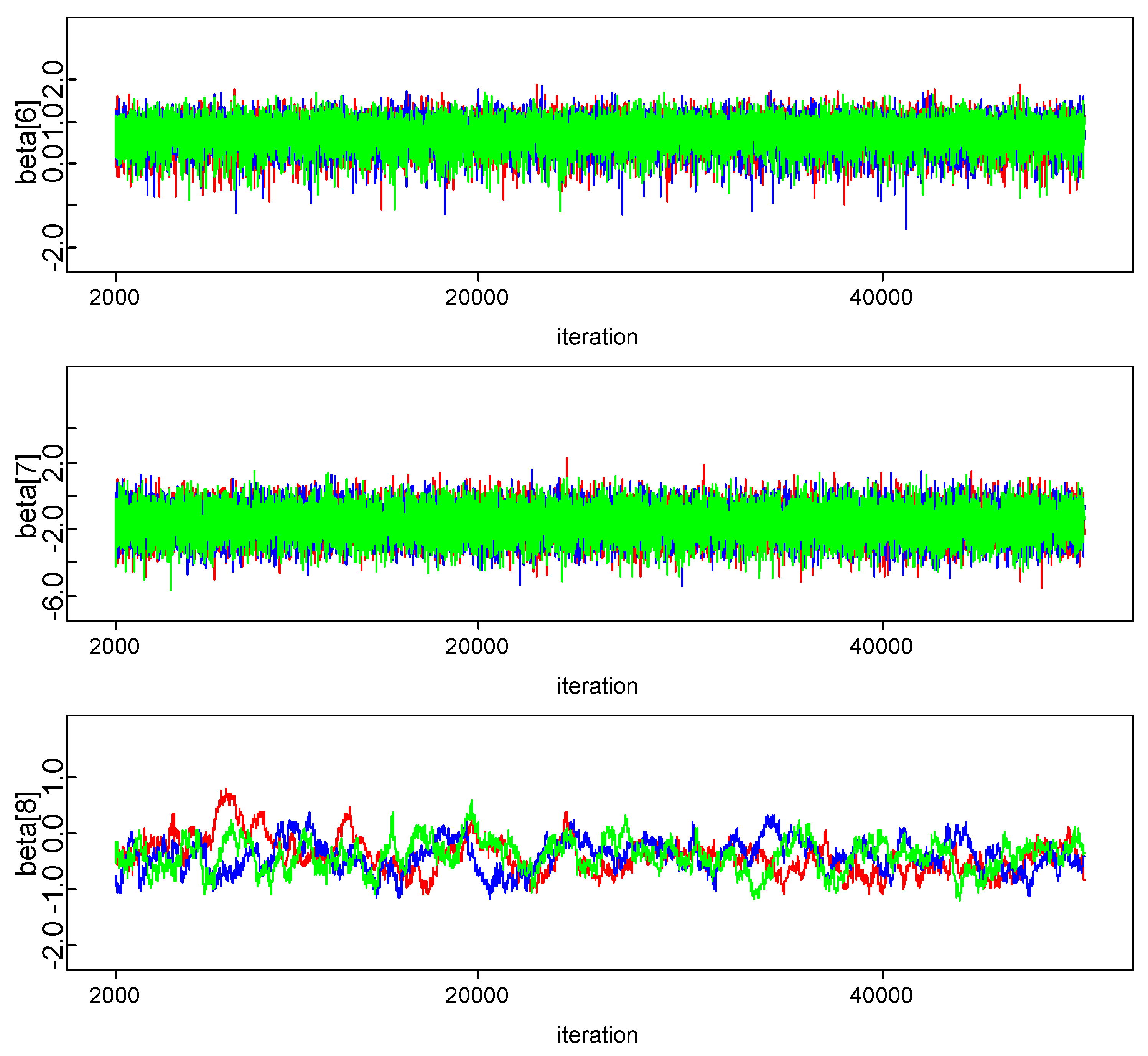
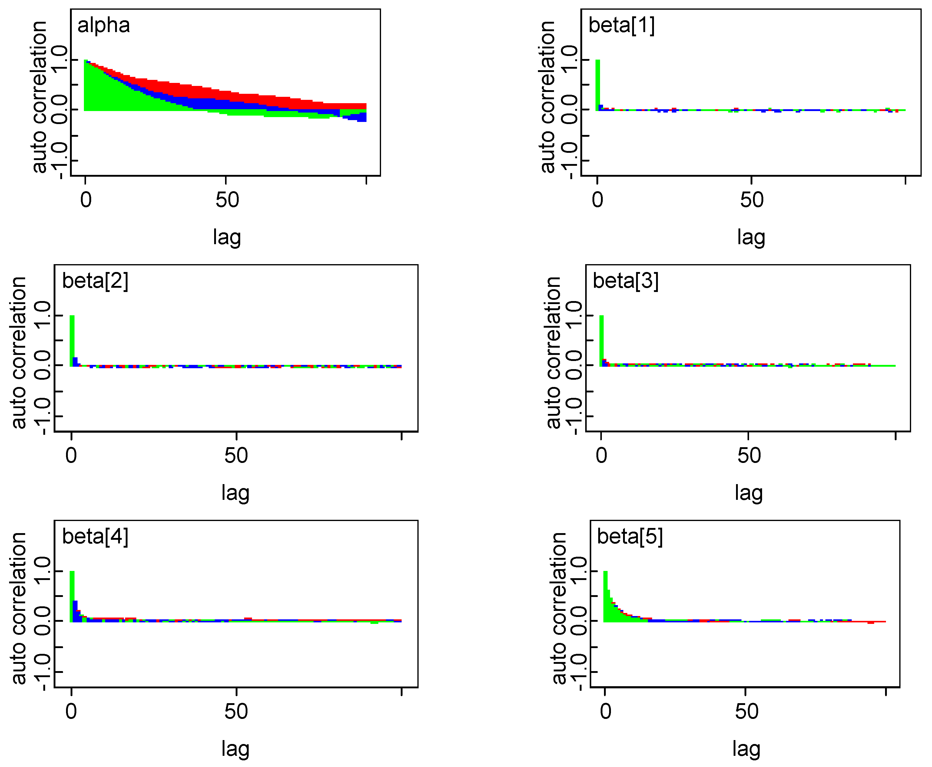
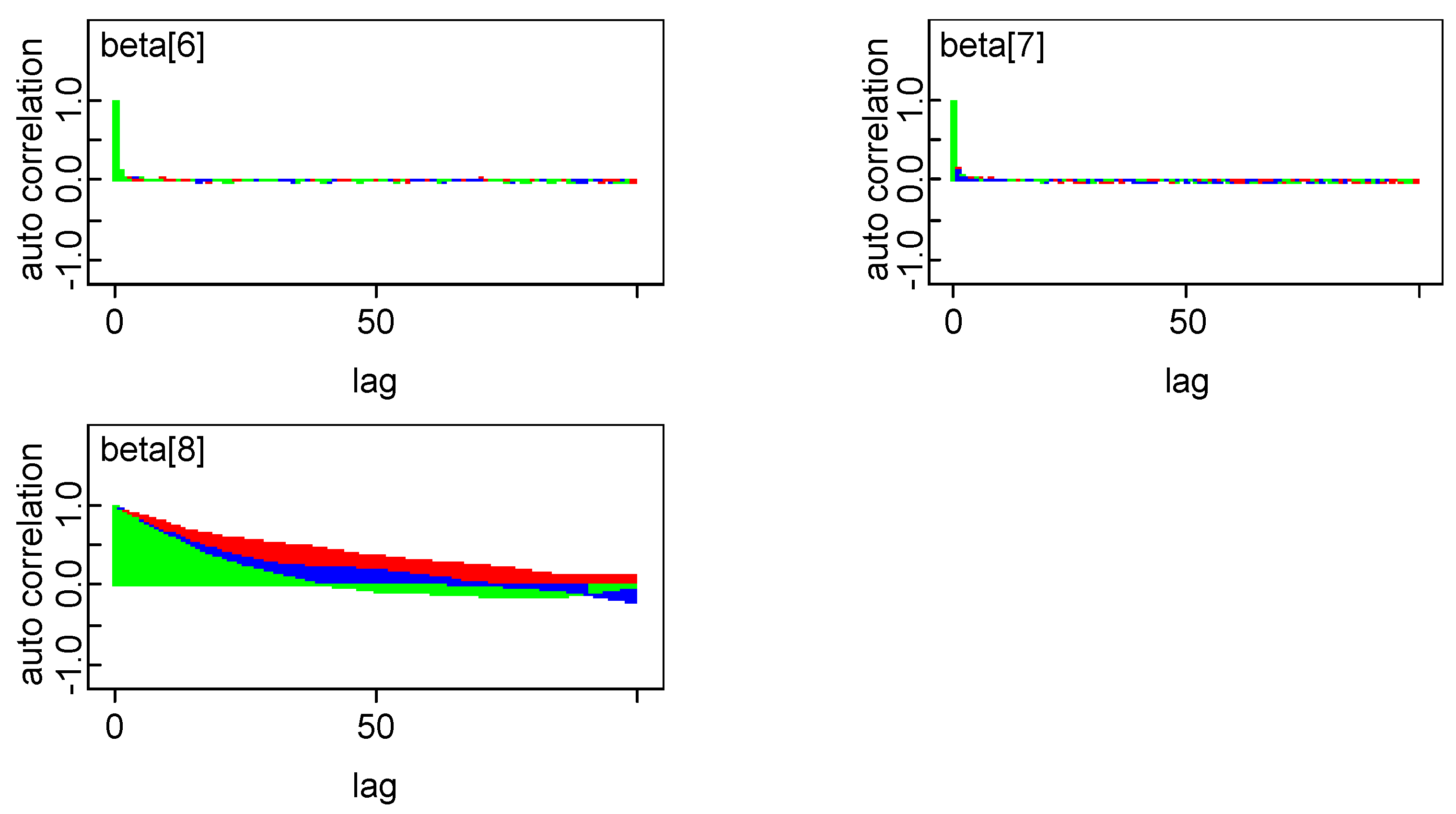
In order to estimate the parameters of model in Bayesian framework, it is essential to specify prior distributions pertaining to each unknown parameter. A priori regression coefficients are assumed to be following normal distribution. Combination of joint prior distribution with likelihood function leads to joint posterior distribution. The convergence check for three Markov chains has been carried out by observing trace plot showing full history of all parameters, which is found to be satisfactory. One can also make more precise inference about the convergence by observing autocorrelation and the marginal density plot of model parameters. All diagnostics indicate that the parameter chains have converged by 2000 iterations. In our empirical analysis, we have utilized three Markov Chain to increase the speed of convergence and smoothness of the density plot and run 50,000 iterations and discard first 2000 iterations as burn-in sample and select every third sample to overcome autocorrelation of random draws. Remaining draws are used to summarize the posterior density and to conduct Bayesian inference. The kernel density plots, autocorrelation along with trace plots of parameters are shown in Appendix A. Plots indicate that all the parameters of the chain are mixing well with autocorrelation vanishing before 10 lags in each case. Posterior density of parameters is almost converging to normal distribution.

Summary statistics of sampled data and training sample, which contains final variables selected for modeling exercise in training sample is presented in Table 1 and

Table 2. Descriptive Statistic—Entire Sample.

Variable	Category	Mean	SD
EBIT_TAXPAID	0	10.89	35.24
	1	−65.34	227.36
PROFIT_MARGIN	0	0.15	0.11
	1	−0.16	0.29
REAT_EARNING_ASSET	0	0.06	0.05
	1	−0.07	0.12
DEBT_ASST	0	0.13	0.13
	1	0.20	0.21
RECEIVABLE_CURR_ASST	0	0.37	0.24
	1	0.31	0.20
CASH_CURRENT_LIB	0	0.25	0.53
	1	0.11	0.31
WORKING_CAP_ASSET	0	0.13	0.21
	1	−0.03	0.41
LOG_NETWORTH	0	6.07	0.73
	1	5.57	0.65

0 stands for non-distressed whereas 1 depicts distressed firms. Number of non-distressed firms are 3732, whereas number of distressed firms are 244.

respectively. The average values and standard deviation of all selected variables is roughly similar as that of training sample. For training sample, profitability indicators, like profit margin and retained earnings, have average values of 15% and 6% respectively for successful (non-distressed firms). In contrast, profitability measures for distressed firms belong to the band of −16.0% to −6.4%, which clearly indicates distress build-up. Average EBIT to tax ratio for non-distressed companies is 10.7%, although it is recorded as −54.8% for distressed firms. Debt to asset ratio is 13.2% for non-distressed firms, whereas 19.8% for distressed class, which clearly indicates strain. Working capital to assets ratio is calculated as 13.0% and 0.2% for non-distressed and distressed class of firms, respectively. Receivable to current ratio is 37.2% and 31.6%, respectively, for distressed and non-distressed firms.

The Student’s t-test for equality of means was performed to verify the discriminatory power of the proposed criteria to classify companies correctly in distressed and non-distressed classes. The results show that proposed methodology is able to clearly discriminate firms as per explanatory variables.2

4.2. Model Comparison

This section contains a comparison of in sample classification and cross validation prediction ability of standard logistic and Bayesian logistic model. The regression results based on standard and Bayesian logistic model are presented in

Table 3. Logistic estimation result.

Variable	Estimate	SE
Intercept	1.748	1.636
EBIT_TAXPAID	−0.033 **	0.016
PROFIT_MARGIN	−44.665 ***	4.839
REAT_EARNING_ASSET	−6.367 *	3.821
DEBT_ASSET	4.368 ***	1.254
RECEIVABLE_CURR_ASSET	−2.199 **	0.914
CASH_CURRENT_LIB	0.809 ***	0.245
WORKING_CAP_ASSET	−1.598 *	0.861
LOG_NETWORTH	−0.424	0.281
Model Diagnostics
−2 Log likelihood	247.167
Nagelkerke R square	0.845
Iterations	10

*, **, *** indicate significance at 10%, 5% and 1% level respectively.

and

Table 4. Bayesian logistic estimation result.

Variable	Mean	SD
Intercept	1.636	0.296
EBIT_TAXPAID	−0.038 **	1.719
PROFIT_MARGIN	−45.59 ***	0.016
REAT_EARNING_ASSET	−7.114 *	4.982
DEBT_ASSET	4.448 ***	4.066
RECEIVABLE_CURR_ASSET	−2.315 **	1.29
CASH_CURRENT_LIB	0.724 **	0.925
WORKING_CAP_ASSET	−1.642 *	0.32
LOG_NETWORTH	−0.400	0.88

*, **, *** indicate significance at 10%, 5% and 1% level respectively.

, respectively. Probability of default is explained by many variables, most of which are found to be statistically significant also. The regression results that are based on standard logistic model and Bayesian logistic model are quite similar, however varying in terms of magnitude and dispersion.

EBITDA to tax ratio has negative impact on distress thereby lowering default probability. Profitability measures viz., profit margin and retained earnings to assets ratios have inverse impact on distress for both Normal and Bayesian logit model. The leverage ratio i.e., debt to asset ratio indicates positive association with distress. Working capital ratio displays a negative relationship with probability of distress. It implies that efficient working capital management plays beneficial role to enhance firm’s profitability. Similarly, high receivables are resulting in lowering of distress. High receivables imply greater liquid resources at the disposal of firm, which is also leading to reduction of distress level. Size as captured by log of net worth measures firms’ financial health, is negatively associated with probability of default in both modeling frameworks.

Table 5. Standard logit model—classification table.

Observed	Predicted		Percentage Correct
	Non-Distressed	Distressed
Non-Distressed	2433	9	99.6
Distressed	27	150	84.7
Overall Percentage			98.6

and

Table 6. Bayesian logit model—classification table.

Observed	Predicted		Percentage Correct
	Non-Distressed	Distressed
Non-Distressed	2435	7	99.7
Distressed	23	154	87.0
Overall Percentage			98.9

tabulate the percentage of correct classifications for logistic and Bayesian logistic model, respectively. The in-sample classification accuracy results reveal Bayesian logistic correctly classifying 98.9% firms as compared to 98.6% by the standard logistic model.

The ROC curve that gauges predictive ability of models has also been plotted and it shows a higher area under curve in case of Bayesian logistic i.e., 98.9% in contrast to 98.6% obtained employing standard logit model (Figure 1). The results show Bayesian logistic model to be more accurate in terms of correctly classifying firms.

4.3. Predictive Ability of Model

Prediction has also been carried out to assess the overall performance and efficiency of the model. N period ahead prediction is performed based on the model obtained on the training sample. The predictions have been done for both different cut values for within-sample and for testing sample separately.

Table 7. Predictions for varied cut values (%).

Cut Value	Training Sample				Testing Sample
	Distress Prediction	Non-Distress Prediction	Type I Error	Type II Error	Distress Prediction	Non-Distress Prediction	Type I Error	Type II Error
0.1	93.8	96.9	6.2	3.1	92.5	97.2	7.5	2.8
0.2	91.5	98.4	8.5	1.6	89.6	98.5	10.4	1.5
0.3	88.1	98.9	11.9	1.1	86.6	98.8	13.4	1.2
0.4	87.6	99.5	12.4	0.5	83.6	99.1	16.4	0.9
0.5	84.7	99.6	15.3	0.4	82.1	99.2	17.9	0.8
0.6	80.8	99.8	19.2	0.2	80.6	99.3	19.4	0.7
0.7	77.4	99.9	22.6	0.1	76.1	99.5	23.9	0.5
0.8	74.6	100	25.4	0.0	73.1	99.5	26.9	0.5
0.9	68.4	100	31.6	0.0	67.2	99.5	32.8	0.5

shows predictions that are based on different cut values for both training and testing samples. It is observed that the higher the cut value, the lower the prediction accuracy and higher is Type I error.

The results based on prediction for N period ahead is plotted in Figure 2. It is observed that, as we move farther in time, the Type I error is increasing and correct prediction of distressed firms is falling. It is noted that in fifth period ahead the Type I error rises to as high as 40%.

5. Conclusions

There exist three major objectives of this study. Firstly, it examines determinants of firm distress. Secondly, it develops a Bayesian logistics framework for distress prediction, whose performance is evaluated with standard logistic model. Finally, it carries out model prediction analysis. In this regard, data set based on Indian firms extracted from Capital IQ has been utilized.

Since, in the Indian context, bankruptcy details of firms are not available, therefore, an efficient methodology has been developed to classify the firms as distressed or non-distressed. It enables capturing incipient signs of distress for Indian firms. Additionally, it enables enlarging the sample of distressed firms thereby leading to robust outcome. Once the classification has been completed, whole data set has been divided into two groups viz., training and testing samples, removing outlier firms. This is one of the foremost studies that has developed methodology to classify firms into distress and non-distress class and examined it for Indian firms. Results suggest that the Bayesian methodology performs well, not only in terms of model parameters and accuracy in terms of reduced error, but it has also led to greater predictive ability as compared to the classical logistic model. Similarly, when model developed based on testing data set is used to predict the distress of testing samples, the Bayesian logistic model is found to outperform standard logistic model. Consequently, the study contributes by proposing useful outline to signal early distress situation.

References

- Altman, Edward I. 1968. Financial ratios, discriminant analysis and the prediction of corporate bankruptcy. The Journal of Finance 23: 589–609. [Google Scholar] [CrossRef]
- Altman, Edward I., Giancarlo Marco, and Franco Varetto. 1994. Corporate distress diagnosis: Comparisons using linear discriminant analysis and neural networks (the Italian experience). Journal of Banking & Finance 18: 505–29. [Google Scholar]
- Bapat, Varadraj, and Abhay Nagale. 2014. Comparison of Bankruptcy Prediction Models: Evidence from India. Accounting and Finance Research 3: 91. [Google Scholar] [CrossRef]
- Beaver, William H. 1966. Financial ratios as predictors of failure. Journal of Accounting Research 4: 71–111. [Google Scholar] [CrossRef]
- Campbell, John Y., Jens Hilscher, and Jan Szilagyi. 2008. In search of distress risk. The Journal of Finance 63: 2899–939. [Google Scholar] [CrossRef] [Green Version]
- Gepp, Adrian, and Kuldeep Kumar. 2015. Predicting financial distress: A comparison of survival analysis and decision tree techniques. Procedia Computer Science 54: 396–404. [Google Scholar] [CrossRef]
- Li, Zhiyong, Jonathan Crook, and Galina Andreeva. 2013. Chinese Companies Distress Prediction: An Application of Data Envelopment Analysis. Journal of the Operational Research Society. [Google Scholar] [CrossRef]
- Lin, S. M., Jake Ansell, and Galina Andreeva. 2012. Predicting default of a small business using different definitions of financial distress. Journal of the Operational Research Society 63: 539–48. [Google Scholar] [CrossRef]
- Nam, Chae Woo, Tong Suk Kim, Nam Jung Park, and Hoe Kyung Lee. 2008. Bankruptcy prediction using a discrete-time duration model incorporating temporal and macroeconomic dependencies. Journal of Forecasting 27: 493–506. [Google Scholar] [CrossRef]
- Ohlson, James A. 1980. Financial ratios and the probabilistic prediction of bankruptcy. Journal of Accounting Research 18: 109–31. [Google Scholar] [CrossRef]
- Sheppard, Jerry Paul. 1994. Strategy and bankruptcy: An exploration in to organizational death. Journal of Management 20: 795–883. [Google Scholar]
- Shumway, Tyler. 2001. Forecasting bankruptcy more accurately: A simple hazard model. The Journal of Business 74: 101–24. [Google Scholar] [CrossRef]
- Yang, Zijiang, Wenjie You, and Guoli Ji. 2011. Using partial least squares and support vector machines for bankruptcy prediction. Expert Systems with Applications 38: 8336–42. [Google Scholar] [CrossRef]
- Zellner, Arnold, and Tomohiro Ando. 2010. Bayesian and non-Bayesian analysis of the seemingly unrelated regression model with Student-t errors, and its application for forecasting. International Journal of Forecasting 26: 413–34. [Google Scholar] [CrossRef]
- Zmijewski, Mark E. 1984. Methodological issues related to the estimation of financial distress prediction models. Journal of Accounting Research 22: 59–82. [Google Scholar] [CrossRef]