On Two Mixture-Based Clustering Approaches Used in Modeling an Insurance Portfolio


Abstract
1. Introduction
2. Methodology
2.1. Mixture-Based Clustering for the Ordered Stereotype Model
- Likelihood functions:
- The (incomplete) likelihood of the data iswhere is the probability of the data response defined in Equation (2).We define the unknown row group memberships through the following indicator latent variables,where indicates that row i is in row group g. It follows that (), and, since their a priori row membership probabilities are ,Consequently, the complete data log-likelihood of this model using the known data and the unknown data is as follows:
- Parameter estimation:
- The parameter estimation for a fixed number of components G is performed using the maximum likelihood estimation approach fulfilled by means of the expectation-maximization (EM) algorithm proposed by Dempster et al. (1977) and used in most finite mixture problems discussed by McLachlan and Peel (2004).The EM algorithm consists of two steps: expectation (E-step) and maximization (M-step). As part of the E-step, a conditional expectation of the complete data log-likelihood function is obtained given the observed data and current parameter estimates. In the finite mixture model, the latent data corresponds to the component identifiers. As part of the E-step, the expectation taken with respect to the conditional posterior distribution of the latent data, given the observed data and the current parameter estimates, is referred to as the posterior probability that response comes from the gth mixture component, computed at each iteration of the EM algorithm. The remaining part of the M-step requires finding component-specific parameter estimates by solving numerically the maximum likelihood estimation problem for each of the different component distributions.The E-step and M-step alternate until the relative increase in the log-likelihood function is no bigger than a small pre-specified tolerance value, when the convergence of the EM algorithm is achieved. In order to find an optimal number of components, maximum likelihood estimation is obtained for each number of groups G, and the model is selected based on a chosen model selection criterion.In this model, the EM algorithm performs a fuzzy assignment of rows to clusters based on the posterior probabilities. The EM algorithm is initialized with an estimate of the parameters and proceeds by alternation of the E-step and M-step to estimate the missing data and to update the parameter estimates. In this section, we develop the E-step and M-step for row clustering. This development follows closely Fernández et al. (2016) (Section 3).
- E-Step:
- In the tth iteration of the EM algorithm, the E-Step evaluates the expected values of the unknown classifications conditional on the data and the previous estimates of the parameters . The conditional expectation of the complete data log-likelihood at iteration t is given byThe random variable is Bernoulli distributed, so that , and, applying Bayes’ rule, we obtainFinally, we complete the E-step by substituting the previous expression in the complete data log-likelihood at iteration t expressed in Equation (3),
- M-step:
- The M-step of the EM algorithm is the global maximization of the log-likelihood (4) obtained in the E-step, now conditional on the complete data . For the case of finite mixture models, the updated estimations of the term containing the row-cluster proportions and the one containing the rest of the parameters are computed independently. Thus, the M-step has two separate parts.The maximum-likelihood estimator for the parameter where the data are unobserved isTo estimate the remaining parameters , we must numerically maximize the conditional expectation of the complete data log-likelihood in Equation (3). In the case of row clustering,where the maximization is conditional on the parameter constraints following Equation (1).
2.2. The General Linear Cluster-Weighted Model
- Modeling for and :
- The CWM model is based on the assumption that belongs to the exponential family of distributions that are strictly related to GLMs. The link function in Equation (5) relates the expected value . We are interested in estimation of the vector , so the distribution of is denoted by , where denotes an additional parameter associated with a two-parameter exponential family.The marginal distribution has the following components: and . The first component is modeled as p-variate Gaussian density with mean and covariance matrix as .The marginal density assumes that each finite discrete covariate W is represented as a vector , where is , which has the value s, s.t. , and otherwise.where , , , and , . The density represents the product of q conditionally independent multinomial distributions with parameters , . Considering these assumptions, the model in Equation (7) can be stated asIf the CWM models allow for the conditional distribution to be Binomial or Poisson, then they are referred to as the Binomial CWM or the Poisson CWM, respectively. The CWM are also built to handle Gaussian, log-normal, and gamma distributions of . In the next subsection, we will discuss the parameter estimation of the model in Equation (9).
- Parameter Estimation:
- The EM algorithm discussed in the previous section is used to estimate parameters of this model. Let be a sample of n independent pairs observations drawn from the model in Equation (9). For this sample, the complete data likelihood function, , is given bywhere is the latent indicator variable with , indicating that observation originated from the j-th mixture component, and otherwise.By taking the logarithm of Equation (10), the complete data log-likelihood function, , is expressed asIt follows that, at the t-th iteration, the conditional expectation of Equation (11) on the observed data and the estimates from the -th iteration results inThe idea behind the EM algorithm is to generate a sequence of the estimates from the maximum likelihood estimation starting from an initial solution and iterating it with the following steps until convergence:
- E-step:
- The posterior probability that comes from the g-th mixture component is calculated at the t-th iteration of the EM algorithm as
- M-step:
- The Q-function is maximized with respect to , which is done separately for each term on the right hand side in Equation (9). As a result, the parameter estimates , , , and , are obtained on the -th iteration of the EM algorithm:while the estimates of are computed by maximizing each of the G termsMaximization of Equation (13) is performed by numerical optimization in the R language (R Core Team 2016) in a similar framework as the mixture of generalized linear models are implemented. For additional details about this implementation, the reader is referred to Wedel and De Sabro (1995) and Wedel (2002).
2.3. Model Selection Criterion
3. Application
3.1. Data
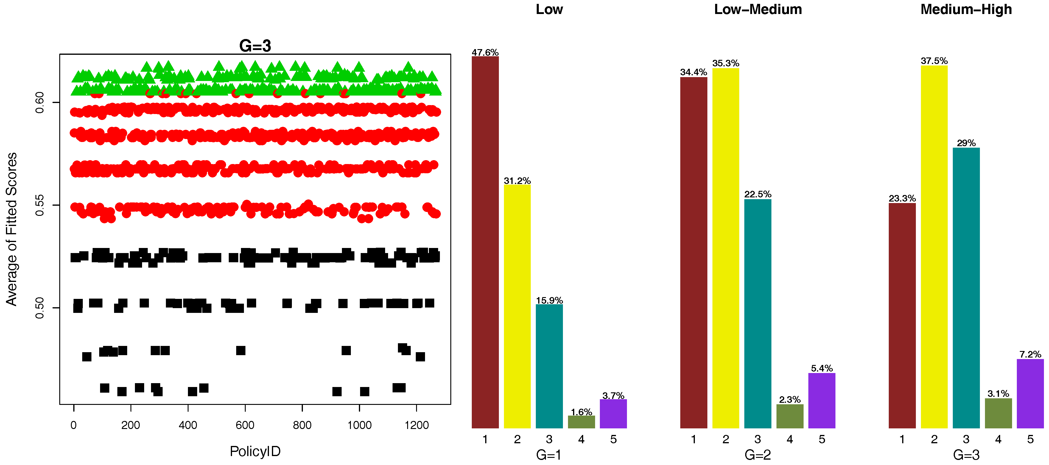
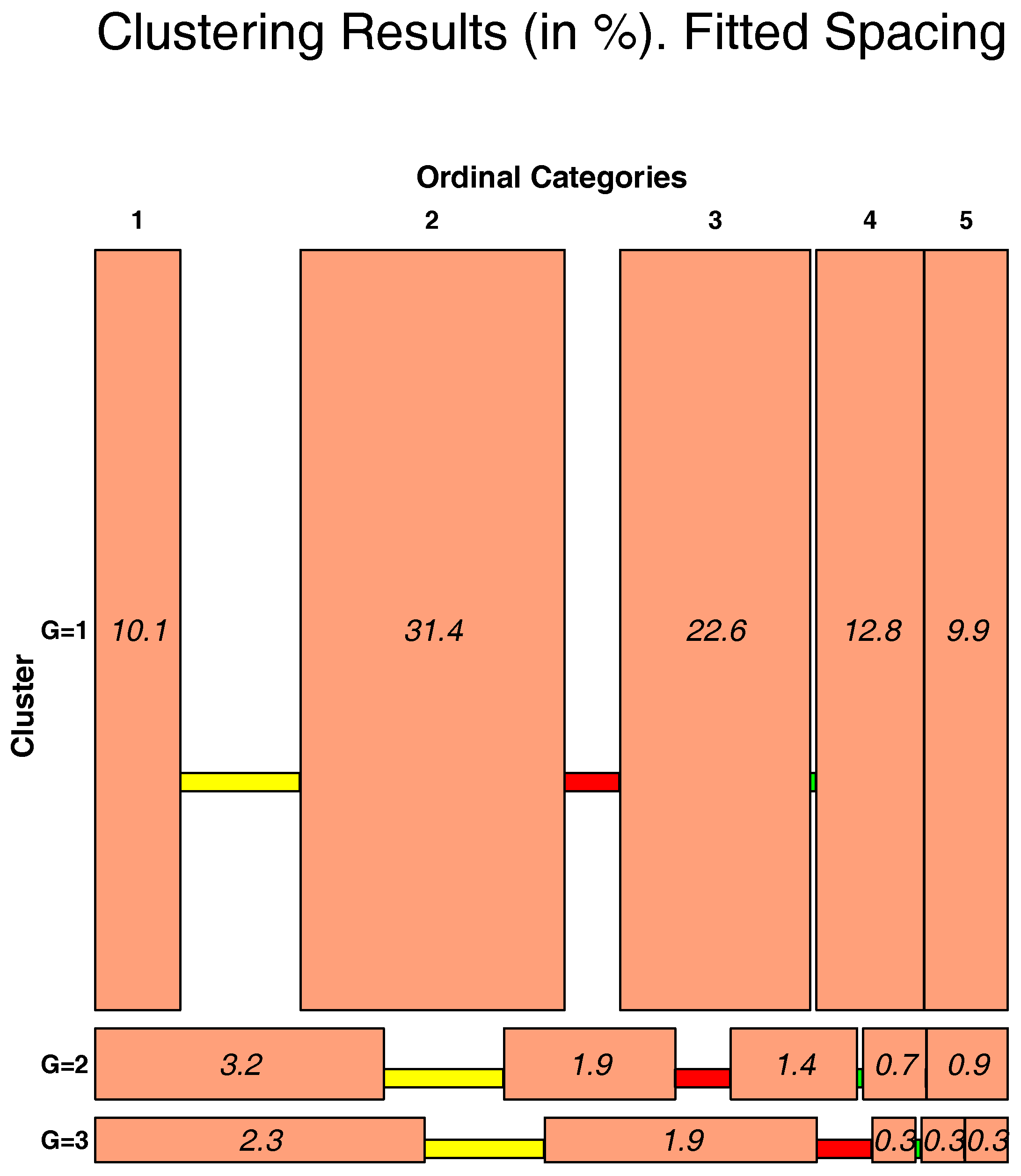
3.2. OSM Results
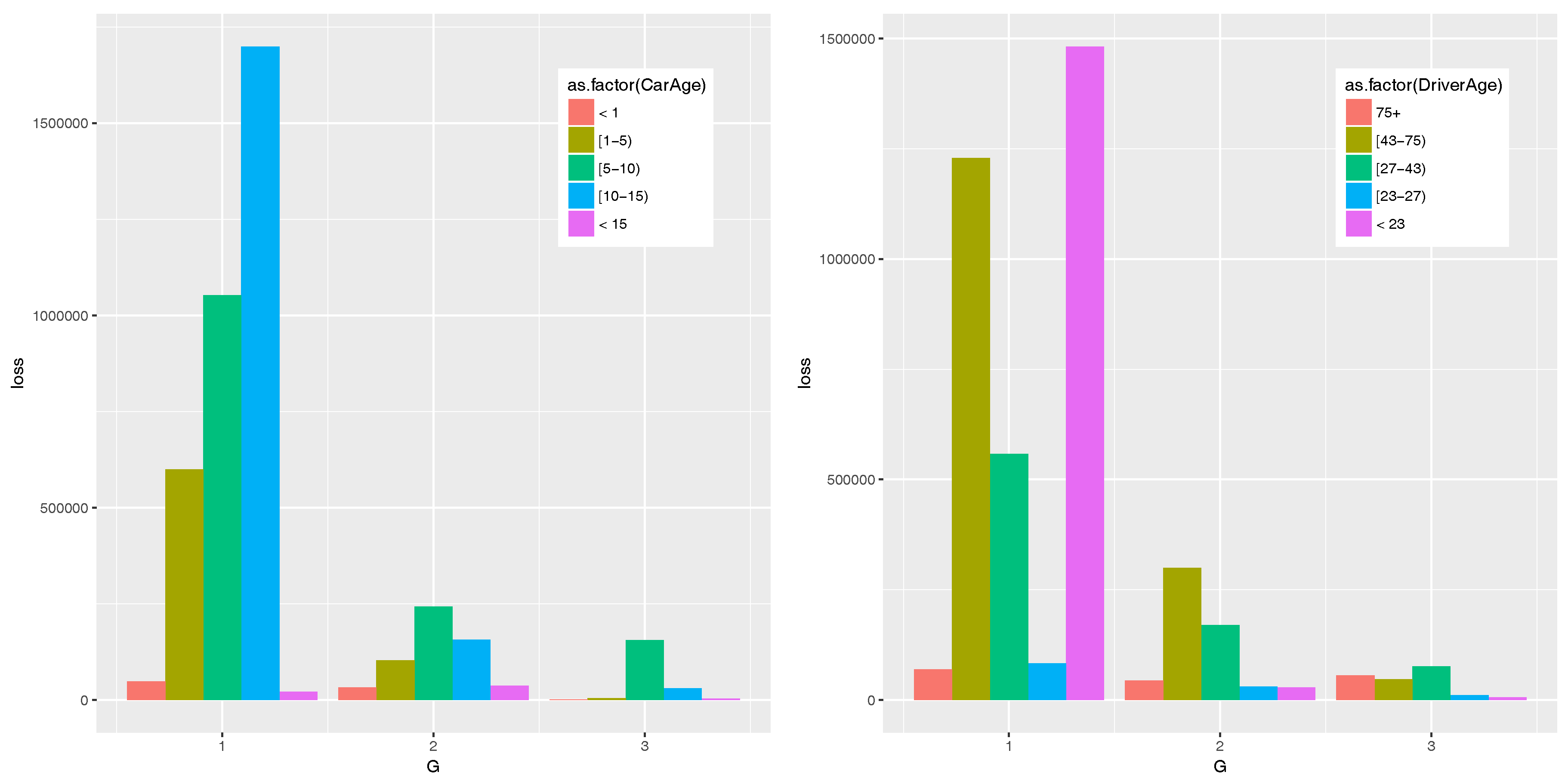
3.3. CWM Results
4. Conclusions
Author Contributions
Acknowledgments
Conflicts of Interest
Appendix A. Model Fitting

| Coefficient | Estimation | S.E. | 95% C.I. |
|---|---|---|---|
| 0.551 | 0.148 | (0.261, 0.841) | |
| −0.219 | 0.171 | (−0.554, 0.116) | |
| 2.533 | 0.224 | (2.094, 2.972) | |
| −1.702 | 0.160 | (−2.016, −1.388) | |
| 1.096 | 0.210 | (0.684, 1.508) | |
| 0.044 | 0.125 | (−0.201, 0.289) | |
| −2.188 | 0.143 | (−2.468, −1.908) | |
| −2.631 | 0.199 | (−3.021, −2.241) | |
| −0.002 | 0.190 | (−0.374, 0.370) | |
| 1.673 | 0.172 | (1.336, 2.010) | |
| 3.636 | 0.209 | (3.226, 4.046) | |
| 4.855 | 0.193 | (4.477, 5.233) | |
| 4.990 | 0.154 | (4.688, 5.292) |
| Cluster 1 | ||||
|---|---|---|---|---|
| Coefficient | Estimation | S.E. | p-Value | |
| Intercept | <2.2×10 | *** | ||
| DriverAge2 | ||||
| DriverAge3 | ||||
| DriverAge4 | ||||
| DriverAge5 | . | |||
| CarAge2 | ||||
| CarAge3 | ||||
| CarAge4 | ||||
| CarAge5 | . | |||
| Density | 5.008×10 | *** | ||
| Exposure | 4.332×10 | *** | ||
| Cluster 2 | ||||
| Coefficient | Estimation | S.E. | p-Value | |
| Intercept | <2.2×10 | *** | ||
| DriverAge2 | ** | |||
| DriverAge3 | * | |||
| DriverAge4 | ||||
| DriverAge5 | ||||
| CarAge2 | ||||
| CarAge3 | * | |||
| CarAge4 | . | |||
| CarAge5 | ||||
| Density | 3.2818×10 | 3.0435×10 | ||
| Exposure | ||||
| Cluster 3 | ||||
| Coefficient | Estimation | S.E. | p-Value | |
| Intercept | <2.2×10 | *** | ||
| DriverAge2 | 8.84×10 | *** | ||
| DriverAge3 | <2.2×10 | *** | ||
| DriverAge4 | <2.2×10 | *** | ||
| DriverAge5 | <2.2×10 | *** | ||
| CarAge2 | ** | |||
| CarAge3 | <2.2×10 | *** | ||
| CarAge4 | <2.2×10 | *** | ||
| CarAge5 | <2.2×10 | *** | ||
| Density | 1.7878×10 | 4.3673×10 | 4.520×10 | *** |
| Exposure | 6.2711×10 | |||
Appendix B. Average Scores for Scatter Plots
References
- Agresti, Alan. 2010. Analysis of Ordinal Categorical Data, 2nd ed. Wiley Series in Probability and Statistics. New York: Wiley. [Google Scholar]
- Akaike, Hirotugu. 1974. A new look at the statistical model identification. IEEE Transactions on Automatic Control 19: 716–23. [Google Scholar] [CrossRef]
- Anderson, John A. 1984. Regression and ordered categorical variables. Journal of the Royal Statistical Society Series B (Methodological) 46: 1–30. [Google Scholar]
- Baribeau, Annmarie Geddes. 2016. Predictive modeling: The quest for data gold. Actuarial Review. Available online: https://www.casact.org/pubs/New-AR/AR_Nov-Dec_2016.pdf (accessed on 7 March 2018).
- Bermúdez, Lluís, and Dimitris Karlis. 2012. A finite mixture of bivariate poisson regression models with an application to insurance ratemaking. Computational Statistics & Data Analysis 56: 3988–99. [Google Scholar]
- Böhning, Dankmar, Wilfried Seidel, Marco Alfò, Bernard Garel, Valentin Patilea, and Günther Walther. 2007. Advances in mixture models. Computational Statistics & Data Analysis 51: 5205–10. [Google Scholar]
- Brown, Garfield O., and Winston S. Buckley. 2015. Experience rating with poisson mixtures. Annals of Actuarial Science 9: 304–21. [Google Scholar] [CrossRef]
- Charpentier, Arthur. 2014. Computational Actuarial Science with R. Boca Raton: CRC Press. [Google Scholar]
- Chen, Lien-Chin, Philip S. Yu, and Vincent S. Tseng. 2011. A weighted fuzzy-based biclustering method for gene expression data. International Journal of Data Mining and Bioinformatics 5: 89–109. [Google Scholar] [CrossRef] [PubMed]
- Dempster, Arthur P., Nan M. Laird, and Donald B. Rubin. 1977. Maximum likelihood from incomplete data via the EM-algorithm. Journal of the Royal Statistical Society B 39: 1–38. [Google Scholar]
- Dutang, Christophe, and Arthur Charpentier. 2016. CASdatasets, R package version 1.0-6; Available online: http://cas.uqam.ca/ (accessed on 6 March 2018).
- Everitt, Brian S., Morven Leese, and Sabine Landau. 2001. Cluster Analysis, 4th ed. London: Hodder Arnold Publication. [Google Scholar]
- Fernández, Daniel, Richard Arnold, and Shirley Pledger. 2016. Mixture-based clustering for the ordered stereotype model. Computational Statistics & Data Analysis 93: 46–75. [Google Scholar]
- Fernández, Daniel, Shirley Pledger, and Richard Arnold. 2014. Introducing Spaced Mosaic Plots. Research Report Series 14-3; Wellington: School of Mathematics, Statistics and Operations Research, VUW. ISSN 1174-2011. [Google Scholar]
- Fraley, Chris, and Adrian E. Raftery. 2002. Model-based clustering, discriminant analysis and density estimation. Journal of the American Statistical Association 97: 611–31. [Google Scholar] [CrossRef]
- Garrido, José, Christian Genest, and Juliana Schulz. 2016. Generalized linear models for dependent frequency and severity of insurance claims. Insurance: Mathematics and Economics 70: 205–15. [Google Scholar] [CrossRef]
- Gershenfeld, Neil. 1997. Nonlinear inference and cluster-weighted modeling. Annals of the New York Academy of Sciences 808: 18–24. [Google Scholar] [CrossRef]
- Green, Peter J. 1995. Reversible jump Markov chain Monte Carlo computation and Bayesian model determination. Biometrika 82: 711–32. [Google Scholar] [CrossRef]
- Grün, Bettina, and Friedrich Leisch. 2008. Finite Mixtures of Generalized Linear Regression Models. Berlin: Springer. [Google Scholar]
- Hubert, Lawrence, and Phipps Arabie. 1985. Comparing partitions. Journal of Classification 2: 193–218. [Google Scholar] [CrossRef]
- Ingrassia, Salvatore, Antonio Punzo, Giorgio Vittadini, and Simona C. Minotti. 2015. The Generalized Linear Mixed Cluster-Weighted Model. Journal of Classification 32: 85–113. [Google Scholar] [CrossRef]
- Jobson, John D. 1992. Applied Multivariate Data Analysis: Categorical and Multivariate Methods. Springer Texts in Statistics. Berlin: Springer. [Google Scholar]
- Johnson, Stephen C. 1967. Hierarchical clustering schemes. Psychometrika 2: 241–54. [Google Scholar] [CrossRef]
- Kaufman, Leonard, and Peter J. Rousseeuw. 1990. Finding Groups in Data an Introduction to Cluster Analysis. New York: Wiley. [Google Scholar]
- Klugman, Stuart, and Jacques Rioux. 2006. Toward a unified approach to fitting loss models. North American Actuarial Journal 10: 63–83. [Google Scholar] [CrossRef]
- Kraskov, Alexander, Harald Stögbauer, Ralph Gregor Andrzejak, and Peter Grassberger. 2005. Hierarchical clustering using mutual information. EPL (Europhysics Letters) 70: 278–84. [Google Scholar] [CrossRef]
- Lee, Simon C. K., and X. Sheldon Lin. 2010. Modeling and evaluating insurance losses via mixtures of Erlang distributions. North American Actuarial Journal 14: 107–30. [Google Scholar] [CrossRef]
- Lewis, S. J. G., Thomas Foltynie, Andrew D. Blackwell, Trevor W. Robbins, Adrian M. Owen, and Roger A. Barker. 2003. Heterogeneity of parkinson’s disease in the early clinical stages using a data driven approach. Journal of Neurology, Neurosurgery and Psychiatry 76: 343–48. [Google Scholar] [CrossRef] [PubMed]
- Liu, Ivy, and Alan Agresti. 2005. The analysis of ordered categorical data: An overview and a survey of recent developments. TEST: An Official Journal of the Spanish Society of Statistics and Operations Research 14: 1–73. [Google Scholar] [CrossRef]
- Manly, Bryan F.J. 2005. Multivariate Statistical Methods: A Primer. Boca Raton: Chapman & Hall/CRC Press. [Google Scholar]
- Mazza, Angelo, Antonio Punzo, and Salvatore Ingrassia. 2017. flexCWM, R package version 1.7; Available online: https://cran.r-project.org/web/packages/flexCWM/index.html (accessed on 6 March 2018).
- McCullagh, Peter. 1980. Regression models for ordinal data. Journal of the Royal Statistical Society 42: 109–42. [Google Scholar]
- McCullagh, Peter, and John A Nelder. 1989. Generalized Linear Models, 2nd ed. London: Chapman & Hall. [Google Scholar]
- McCune, Bruce, and James B. Grace. 2002. Analysis of Ecological Communities. Gleneden Beach: MjM Software Design, vol. 28. [Google Scholar]
- McLachlan, Geoffrey, and David Peel. 2004. Finite Mixture Models. Hobuken: John Wiley & Sons. [Google Scholar]
- McLachlan, Geoffrey J., and Kaye E. Basford. 1988. Mixture Models: Inference and Applications to Clustering. Statistics, Textbooks and Monographs. New York: M. Dekker. [Google Scholar]
- Meila, Marina. 2005. Comparing clusterings: An axiomatic view. Paper presented at the 22nd International Conference on Machine Learning (ICML 2005), Bonn, Germany, August 7–11; pp. 577–84. [Google Scholar]
- Melnykov, Volodymyr, and Ranjan Maitra. 2010. Finite mixture models and model-based clustering. Statistics Surveys 4: 80–116. [Google Scholar] [CrossRef]
- Miljkovic, Tatjana, and Bettina Grün. 2016. Modeling loss data using mixtures of distributions. Insurance: Mathematics and Economics 70: 387–96. [Google Scholar] [CrossRef]
- Miljkovic, T. 2017. Computational Actuarial Science With R. Journal of Risk and Insurance 84: 267. [Google Scholar]
- Nelder, John Ashworth, and Robert W. M. Wedderburn. 1972. Generalized linear models. Journal of the Royal Statistical Society Series A (General) 135: 370–84. [Google Scholar] [CrossRef]
- Pledger, Shirley, and Richard Arnold. 2014. Multivariate methods using mixtures: Correspondence analysis, scaling and pattern-detection. Computational Statistics and Data Analysis 71: 241–61. [Google Scholar] [CrossRef]
- Quinn, Gerry P., and Michael J. Keough. 2002. Experimental Design and Data Analysis for Biologists. Cambridge: Cambridge University Press. [Google Scholar]
- Team, R. Core. 2016. R: A Language and Environment for Statistical Computing. Vienna: R Foundation for Statistical Computing. [Google Scholar]
- Schwarz, Gideon. 1978. Estimating the dimension of a model. The Annals of Statistics 6: 461–64. [Google Scholar] [CrossRef]
- Shi, Peng, Xiaoping Feng, and Anastasia Ivantsova. 2015. Dependent frequency severity modeling of insurance claims. Insurance: Mathematics and Economics 64: 417–28. [Google Scholar] [CrossRef]
- Verbelen, Roel, Lan Gong, Katrien Antonio, Andrei Badescu, and Sheldon Lin. 2014. Fitting mixtures of Erlangs to censored and truncated data using the EM algorithm. ASTIN Bulltin 45: 729–58. [Google Scholar] [CrossRef]
- Wedel, Michel. 2002. Concominat variables in finite mixture modeling. Statistica Neerlandica 56: 362–75. [Google Scholar] [CrossRef]
- Wedel, Michel, and Wayne S. DeSarbo. 1995. A mixture likelihood approach for generalized linear models. Journal of Classification 12: 21–55. [Google Scholar] [CrossRef]
- Werner, Geoff, and Claudine Modlin. 2016. Basic Ratemaking. Arlington: Casualty Actuarial Society. [Google Scholar]
- Wu, Han-Ming, ShengLi Tzeng, and Chun-houh Chen. 2007. Matrix visualization. In Handbook of Data Visualization. Berlin: Springer, pp. 681–708. [Google Scholar]
- Wu, Xindong, Vipin Kumar, J. Ross Quinlan, Joydeep Ghosh, Qiang Yang, Hiroshi Motoda, Geoffrey J. McLachlan, Angus Ng, Bing Liu, Philip S. Yu, and et al. 2008. Top 10 algorithms in data mining. Knowledge and Information Systems 14: 1–37. [Google Scholar] [CrossRef]


| CWM | |
| Variable Name | Description with Categorical Levels in Parenthesis |
| Driver Age | <23 (1), [23, 27) (2), [27, 43) (3), [43, 75) (4), and [75+ (5) |
| Car Age | <1 (1), [1, 5) (2), [5, 10) (3), [10, 15) (4), and 15+ (5) |
| Density | continuous |
| Exposure | continuous |
| Losses | continuous |
| OSM | |
| Variable Name | Description with Ordinal Levels in Parenthesis |
| Driver Age | <23 (5), [23, 27) (4), [27, 43) (3), [43, 75) (2), and [75+ (1) |
| Car Age | <1 (1), [1, 5) (2), [5, 10) (3), [10, 15) (4), and 15+ (5) |
| Exposure | <0.25 (1), [0.25, 0.50) (2), [0.50, 0.75) (3), [0.75, 1.00) (4), and >1.00+(5) |
| Density | <40 (1), [40, 200) (2), [200, 500) (3), [500, 4500) (4), and 4500+ (5) |
| Losses | <1000 (1), [1000, 2000) (2), [2000, 50,000) (3), [50,000, 100,000) (4), and 100,000+ (5) |
| G | Loglik | AIC | BIC |
|---|---|---|---|
| 1 | −12,155 | 24,453 | 24,599 |
| 2 | −12,081 | 24,188 | 24,276 |
| 3 | −11,777 | 23,584 | 23,685 |
| 4 | −12,773 | 25,580 | 25,695 |
| 5 | −12,851 | 25,641 | 25769 |
| G | Loss | Driver Age | Exposure | Car Age | Density |
|---|---|---|---|---|---|
| 1 | |||||
| 2 | |||||
| 3 |
| G | Loglik | AIC | BIC |
|---|---|---|---|
| 1 | −12,495 | 25,025 | 25,112 |
| 2 | −11,956 | 23,229 | 23,394 |
| 3 | −11,064 | 22,222 | 22,464 |
| 4 | −10,801 | 22,200 | 22,519 |
© 2018 by the authors. Licensee MDPI, Basel, Switzerland. This article is an open access article distributed under the terms and conditions of the Creative Commons Attribution (CC BY) license (http://creativecommons.org/licenses/by/4.0/).
Share and Cite
Miljkovic, T.; Fernández, D. On Two Mixture-Based Clustering Approaches Used in Modeling an Insurance Portfolio. Risks 2018, 6, 57. https://doi.org/10.3390/risks6020057
Miljkovic T, Fernández D. On Two Mixture-Based Clustering Approaches Used in Modeling an Insurance Portfolio. Risks. 2018; 6(2):57. https://doi.org/10.3390/risks6020057
Chicago/Turabian StyleMiljkovic, Tatjana, and Daniel Fernández. 2018. "On Two Mixture-Based Clustering Approaches Used in Modeling an Insurance Portfolio" Risks 6, no. 2: 57. https://doi.org/10.3390/risks6020057
APA StyleMiljkovic, T., & Fernández, D. (2018). On Two Mixture-Based Clustering Approaches Used in Modeling an Insurance Portfolio. Risks, 6(2), 57. https://doi.org/10.3390/risks6020057