Price and Profit Optimization for Financial Services


1
Department of Econometrics, Riskcenter-IREA, Universitat de Barcelona, Av. Diagonal, 690, 08034 Barcelona, Spain
2
Cass Business School, City, University of London, 106 Bunhill Row, London EC1Y 8TZ, UK
*
Author to whom correspondence should be addressed.
Risks 2018, 6(1), 9; https://doi.org/10.3390/risks6010009
Submission received: 6 January 2018
/
Revised: 30 January 2018
/
Accepted: 6 February 2018
/
Published: 8 February 2018
Abstract
:Prospective customers of financial and insurance products can be targeted based on the profit the provider expects to earn from them. We present a model for individual expected profit and two alternatives for calculating optimal personalized prices that maximize the expected profit. For one of these alternatives, we obtain a closed-form expression for the price offered to each prospective customer; for the other, we need to use a numerical approximation. In both approaches, the profits generated by prospective customers are not immediately observed, given that the products sold by these companies have a risk component. We assume that willingness to pay is heterogeneous and apply our methodology using real data from a European insurance company. Our study indicates that a substantial boost in profits can be expected when applying the simplest optimal pricing method proposed.
1. Introduction
Financial service providers can maximize their expected profits by fine-tuning the price of their products. Here, we address the problem that banks and insurance companies face as they seek to fix a price that is high enough to cover potential risk yet low enough to attract customers. We present and compare two optimization strategies: the first involves identifying the optimal personalized price discount on a closed-form expression, which permits a straightforward implementation; the second is based on a numerical optimization procedure.
Profit maximization is a challenge, dependent on a company’s specific knowledge of the probability of a sale, the cost of a sale attempt, and the expected profit once a sale has been made. Here, we propose extending this general approach by introducing price personalization. To do so, we approximate each customer’s reaction to a price increase/decrease and from this derive an expression for the optimal price at which a product should be sold to maximize the expected profit, accounting at the same time for the possibility that the customer will not buy the product if the price is too high. Customer reactions to changes in price, i.e., their price elasticity, are known to vary, and their willingness to pay is not the same. We then compare this optimal pricing approach with a strategy that requires no assumption about price elasticity but which is not a one-step formula.
We present a real case study conducted within the motor insurance sector. We made a purchase offer (i.e., the price given to a prospective customer by a member of the sales staff for a specific product) to a sample of potential motor insurance clients, some of whom were given a modified price so that we could study their response. During data collection, the experiment was constructed in such a way that a purchase offer was associated with a change in price, which neither the sales staff nor the prospective customers were aware of. This means the price change can be considered as being independent of any characteristics of the individual, and we can compare the purchase probability of individuals offered different prices and calculate the average price elasticity for this specific motor insurance product. The data set also contains descriptive information about the prospective customers and the vehicles to be insured. As usual, we divide the data into a training and a test sample. In the first sample, we estimate the components of our expected profit formula, and then, in the test sample, we compare the implementation of the two optimization strategies.
Even if we do not present the theoretical background of this paper, we need to mention the topic of perfect competition and the role of prices in a competitive market. Companies apparently look at things in the same way, but they still have different prices, and these pricing differentials do not compete away. Not all companies operate with the same costs, so they have to charge customers for that; moreover, there is imperfect information when assessing the level of risk to be covered because some factors are difficult to measure. For example, in motor insurance, aggressiveness and driving style are examples of such risk factors.
Our work only considers risk-related variables to set prices. We do not discuss here if some jurisdictions could allow rates that depend on variables not related to loss costs. The protection of social discrimination on the one hand and the right to profit maximization in a firm on the other are a subject beyond our scope, but social discrimination questions and ethics are of outmost importance. When we use the words “optimal” and “efficient”, we refer to values from the firm’s perspective, but as we will see later, even including age as a potential profit maximization factor, could be controversial. We only give an illustration of the methodology and we do not aim at imposing this particular choice of variables influencing the price. In many US states where underwriting criteria must be mutually exclusive and exhaustive, each insured must fit into exactly one rating cell, and they must all be offered the same price. That would probably make the type of experiment described here impossible (see NAIC’s white paper, (NAIC 2015)).
The rest of this paper is organized as follows. Section 2 reviews the literature on optimal insurance contracts. Section 3 describes our model and sets out its profit expressions. It also discusses optimal pricing and profit maximization strategies. The interplay between theory and practice is explored in Section 4, where the real-data study is presented. The value of pricing strategies is discussed in our conclusions, and directions for future research are identified.
2. Literature Review
The financial services offered by banks and insurance companies (including mortgage contracts and other types of loans; household, car, and motorcycle insurance policies; and other kinds of personal insurance products) differ from conventional retail products and services. First, there is a time gap between the collection of payment and the realization of the cost, which complicates profit calculation. Selling different types of risk transfer products is a paradox from a standard manufacturing point of view, because it is merely a promise to compensate if a particular event occurs. As such, the product is sold before its final cost is known. Second, prices and internal processes are often supervised by authorities to ensure that the providers stay solvent. Third, the costs associated with a risk transfer product may vary greatly: many customers are likely to produce small or no costs for the company, while a few might be associated with extremely high cost payouts.
The pricing of financial services has generated its own specific strand in the academic literature, where extensive coverage has been given to risk assessment, solvency, fair premium calculation (Goovaerts et al. 1984), the design of optimal insurance policies (Rothshild and Stiglitz 1976; Dionne et al. 2000), and, to a lesser degree, insurance purchase and claim decisions (Von Lanzenauer and Wright 1991). However, the identification of potential customers that might be suited to a given type of insurance contract, including possible price reductions or increases, has only been examined in relation to experience rating models (Boucher et al. 2009; Denuit et al. 2007) and purchase probability (Guelman and Guillen 2014). Moreover, the interface between optimal pricing and profit maximization remains largely unexplored.
The insurance marketing literature has turned its attention to the identification of prospective customers. For example, Bult and Wansbeek (1995) base optimal target selection on identifying customers with positive marginal profit. This represents an initial step towards the efficient segmentation of potential customers based on expected profits. However, rather than concentrating on short-term profits, companies can estimate a customer’s lifetime value. Venkatesan and Kumar (2004) define and explore customer lifetime value, employing a model that uses classical regression techniques. Gönül and Hofstede (2006) take this approach further by introducing optimization objectives, such as profit maximization, customer retention and utility maximization. Donnelly et al. (2013) study asymmetric information as part of the pricing scheme. Other studies of customer segmentation address the concept of cross-sellin, and include the notable contributions of (Kamakura et al. 1991, 2003, 2004; Knott et al. 2002; Li et al. 2005, 2010; Kamakura 2007). Cross-market strategies are analyzed by Goié et al. (2011), who conclude that even a strategy of offering discounts redeemable in other firms can produce some revenue by simultaneously increasing price and sales in the source market. Schweidel et al. (2011) observe the same phenomenon in data from a multi-line insurance provider in Denmark, which took into account historical information and anticipated lapses. Guillen et al. (2012) find future profit prospects in a similar context to be very informative (see also Guillen et al. 2011; Guelman et al. 2012). Kaishev et al. (2013) present a profit model specifically designed for products for which the profit consists of a stochastic income at the point of sale, minus the cost of contacting a specific customer and the stochastic cost generated by the customer’s actions. The model is primarily intended for use in the insurance and banking sector, where customers can be associated with losses (claims or loan defaults), thus affecting a company’s profit.
Our methodology differs from that employed by Guelman and Guillen (2014) because, rather than focusing on the probability of renewal or purchase given a price offer, we explicitly derive an optimal price for each customer, knowing that the price has an impact on the probability of renewal.
Recently, Laas et al. (2016) analyse developments in motor insurance pricing in Germany, Austria and Switzerland. They focus on the use of different tariff criteria, on the tools used for market-based and customer-specific pricing, and on the information considered for customer valuation. Eling and Luhnen (2008) previously analysed the periods of market price competition in the German motor insurance market after 1994.
3. Individual Profit as Influenced by Price Elasticity
Our model involves a financial services company that offers K different products. We also consider a set of i = 1, ..., I individuals (prospective customers). The product of interest k could be any risk transfer product, such as an insurance policy, mortgage or credit card. We are interested in the profit (The profit is usually calculated for a one-year period, but this can be extended to a longer period or even to the customer’s lifetime. We use the same notion for profit and its components as in (Guelman and Guillen 2014)), , generated by individual i for product k. This profit is unknown when the product is offered to the client. We assume that the product has not yet been purchased. There is a tariff price. i.e., the actuarial price, for individual i and product , denoted as , which is based on information known to the company about the individual’s risk and the desired level of coverage. This information is denoted as vector . Based on , we are able to calculate the tariff price, which might differ significantly from one individual to another. We introduce a price change parameter for individual and product . This parameter modifies the price, so the price offered is . Note that gives the tariff price, corresponds to a price offered above the tariff price and vice versa for ( is invalid because it would produce a non-positive price).
3.1. The Individual Profit Model
When the company offers product k to individual i with a given price change , the individual’s response (purchase/no purchase) is a Bernoulli random variable that depends on the observed characteristics . Then, its expected value is , i.e., the probability of selling product k to individual i when the change in price is equal to . When there is no price change, , then the probability of selling equals . We assume that every sales attempt is associated with a deterministic and constant cost , indifferent to whether or not the contacted customer purchases the product. This cost represents the costs of staffing and administrating the sales department. If the product is sold, then the individual will be associated with a stochastic severity , which is typical of financial service products and can be either the cost of loan defaults or the cost of insurance claims, depending on the type of financial business the company is involved in.
We use the concept of point price elasticity defined as
Expression (1) provides the value of price elasticity when data on an individual’s response to a price change are available.
We assume that an individual’s response to a sales attempt is related to the price change and the price elasticity involved, but not to the tariff price. We also assume that it is independent of the severity, which can only be observed later in time. Drawing on the model developed by Kaishev et al. (2013), here, we propose an extended version that takes the price elasticity into account. The expected profit associated with individual i for product is
The model developed by Kaishev et al. (2013) is a special case of (2), where .
3.2. Model Estimation
Without loss of generality, we use insurance-specific terminology in what follows. To estimate the expected profit for individual and product in Expression (2), we need to estimate all its components. The tariff price can be obtained using a standard pricing procedure (see Frees and Valdez 2008), given the characteristics of the client and product, . For variable we follow the standard actuarial convention and identify it as the aggregate claims cost
where describes the stochastic number of insurance claims (for individual i) and describes the corresponding monetary size of each of these claims. The expected number of claims and their cost, i.e., and , where and are the link functions, can thus be estimated from a standard number of claims and severity generalized linear models. Finally, we obtain .
We consider two possible approaches to approximate sales probability . First, we assume that all customers have the same elasticity . Under this approach, we estimate a logistic model for (without using any information about price changes) and then find from (1). So, we denote by the resulting probability of purchase.
In practice, the best way to estimate price elasticity is by conducting an experiment with a sample of customers to see how much their purchase probability changes when price change modifies the original tariff price. We expect a price increase to reduce the probability of purchase and a fall in price to increase this probability. However, this change in probability is not necessarily symmetrical.
The second approach to estimate the purchasing probability, which we denote as , is to incorporate the price change directly in the logistic model as follows:
In this second approach, we do not assume a constant elasticity, and implicitly we can derive from (1) using in (5).
In both the logistic formulas above, refers to the j-th characteristic of individual i and product , which influences the propensity to buy, and is the vector of parameters in the logistic models, where J is the total number of characteristics in the model. We have intentionally separated the parameter associated with from the other parameters.
3.3. Optimization of Expected Profit
We are interested in finding the value of the price change parameter specific for each individual, at which the expected profit (2), from that individual, is maximized. Hence, the optimization problem is and our two alternatives for presents us with two different solutions to this problem.
In the case of the first alternative, we are able to derive a closed-form expression for the optimal , which we denote
We can present the following proposition, for which the proof is found in the Appendix A.
Proposition 1.
Under the assumption that , the price change which maximizes in (2) is the following
Note that the optimal price change is bound by . Only in this case is the corresponding probability less than or equal to 1.
A closed-form expression for the maximum expected profit can be obtained by inserting (7) into (2) and, after some rearrangements, it yields
In the case of the second alternative, no closed-form expression can be found, and so we solve this optimization problem numerically. The optimal price change for the second alternative can be expressed as
which corresponds to the maximization of (2) with the sales probability from the second alternative.
4. Real Data Study
We have a large sample of car insurance offers made by a European insurance company during 2012. Only one purchase price is offered to a specific prospective customer for a specific product by one of the sales personnel. The customer’s response to this offer can either be to accept it or reject it. This response is reflected in the data set as a binary variable. The data also contain information about the characteristics of each individual contacted (age, place of residence, driver’s license details, etc.) and the car involved (make, fuel type, age, etc.), as well as the price offered, the tariff price, and the estimated expected claims cost. The data set comprises 154,278 offers, of which 81,854 are associated with a random price test, allowing us to estimate the price elasticity and all the parameters for profit optimization. During the price test experiment, a specific price change was randomly assigned to each price offer of either −5%, 0%, or +5% of the tariff price, thus enabling us to measure the effect of a price change on purchase probability. To the other 72,424 offers, which are not associated with the pricing experiment, we applied the two alternative models for optimal pricing in order to compare their outcomes with respect to the expected total profit.
The random price test is designed in such a way that an individual receives a price change of , , or with approximate probabilities 10%, 80%, and 10%, respectively. The individual is not shown the value resulting from the price test or the tariff price , only the price , where is an estimate of .
For our first approach, from the results presented in Table 1, we estimate the average price elasticity as a weighted average of (1) as
4.1. Parameter Estimation
Our procedure for obtaining parameter estimates is based on the 81,854 records in the data set associated with a random price test. It involves two steps.
Step 1.
Estimating the initial parameters , and .
We assume that the estimated cost of a sales approach is generic for all customer contacts. We obtain the estimate by analyzing cost loadings and overheads, as well as by interviewing sales managers at the company.
An estimated expected cost per customer, is available in the data set. In practice, many insurance companies take the average cost per claim and multiply it by the expected number of claims in a year, based on the characteristics of the vehicle to be insured and the individual’s socio-demographic characteristics. is used to estimate . Note that there is an issue the issue when considering an individual’s assessment of their own risk versus the tariff rate. We do not consider premium loadings here to account for any deviations due to the difficulties to measure risk factors.
The tariff price, , is available in the dataset and is used to estimate .
Step 2.
Estimating the sales probability and .
We use the sample of data for the logistic model for both and , i.e., the 81,854 records that are associated with the random price test. Note that the model for does not include the price change as an explanatory factor even though it is significant; rather, the effect of the price change is captured outside the logistic model (see (4)). A qualitative analysis reveals a mix of both categorical and continuous explanatory factors that describe the behavior of the purchase response. The percentage of price offers that led to a purchase is 9.25% of the data sample. The explanatory factors used in this example are listed here:
- Price change: The price change is a continuous explanatory factor only present in the model for .
- Tariff premium: The tariff premium (in hundreds of euros) is a continuous explanatory factor with minimum, mean and maximum equal to 1.001, 4.038, and 15.000, respectively.
- Age: Age of the person contacted as a categorical factor; ≤40, 41–60, and >60. Sample frequencies are 27.6%, 53.8%, and 18.6%, respectively.
- House: Indicator variables describing whether or not the person owns their home (affirmative for 40.3% in the sample).
- Fuel: The type of fuel the car runs on; petrol or diesel. Sample frequencies are 81.7% and 18.3%, respectively.
In practice, insurers can probably extend this list to other characteristics like territory, occupation, type of vehicle, and so on. The parameter estimates and their corresponding standard errors in parentheses are presented in Table 2, for both model alternatives.
4.2. Profit Maximization and Calculation of Optimal Price Changes
We use the remaining 72,424 records from our data set for the purpose of applying the optimal price changes and the corresponding expected profit from our two optimization alternatives. Our aim is to determine which of the two optimal price change alternatives—(7) or (9)—generates the largest total expected profit. Summary statistics from the price optimization using both alternatives are presented in Table 3. We calculate the expected profit in three pricing scenarios, using (2). The baseline expected profit assumes that no price change has been applied to any individual, while the two alternatives for optimal expected profit and assume that the optimal, and individual specific, price changes and have been considered, respectively. Statistics for the sales probability, for the three pricing scenarios, are also found in Table 3. For instance, under model 2, the maximum optimal price change that is obtained in this sample equals 35.0%, while, for model 1, the maximum in this sample is 46.7%. In this sample, model 2 leads to an average optimal price increase of around 5%, while model 1 leads to an average optima price slight decrease of around 0.8%.
In Table 4, we focus solely on the offers associated with a positive expected profit and give the number of these as well as the sum of the corresponding expected profit for the three pricing scenarios. The closed-formula method based on (4) and (6) is presented in the middle column of Table 4. It provides the best results in terms of the expected total profit (105,425 euros, which is higher than the other two), the number of offers with a positive expected profit (35,692, which is also higher than the other two), and the average expected profit per positive offer (105,425/35,692, which is also higher than the other two). The poorest performance is recorded by the baseline alternative (first column), where no price change is performed. The last column of Table 4 indicates that the numerical optimization with a personalized price change based on (9) does not improve the results of the direct method based on (6).
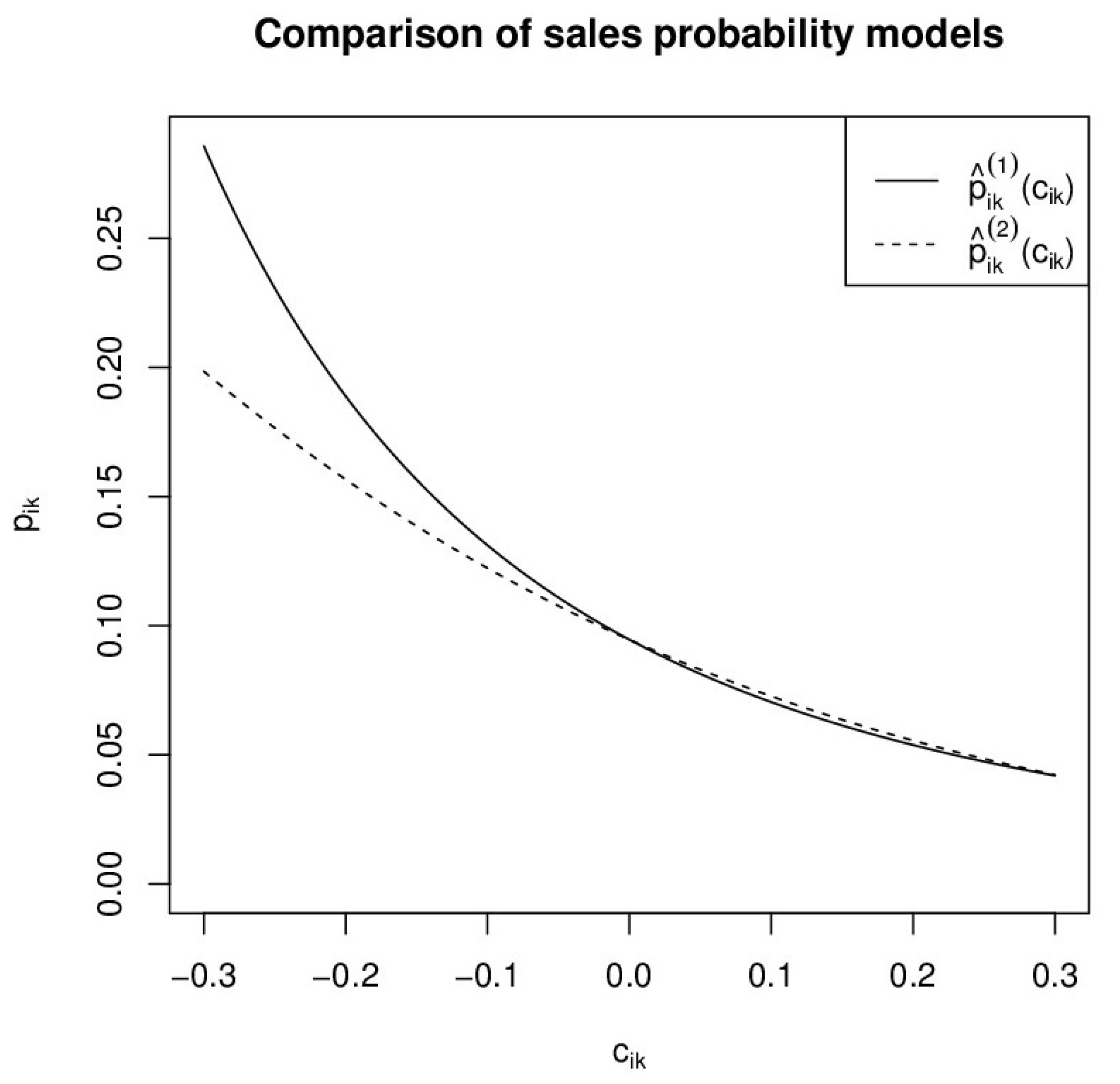
In Figure 1, we present an example of the application of the two sales probability models and for one specific individual offer in the data set and for different values of the price change . For the two alternatives give almost identical sales probability values; however, for , the difference increases as decreases. Figure 1 presents an explanation as to why the first alternative is superior to , with respect to expected total profit. In the case of negative price changes, the first alternative results in higher sales probabilities than with the second alternative, and hence it is associated with higher expected profits. Figure 1 shows only one example of the two models applied to a specific individual offer; however, the general appearance is similar for all cases in the data sample. Note, once more, that we have estimated the price elasticity from price test data between and , hence the effect of any price changes on the sales probability outside this interval has to be extrapolated.
5. Conclusions
In this paper, we have derived two possible pricing methods based on individual-specific optimal price changes and their corresponding optimal profits for financial services. One of the methods expresses the optimal price in a closed-form formula. Our point of departure was the model proposed by Kaishev et al. (2013), which we have generalized for a situation in which the probability of a successful sale attempt depends on the price at which the product is offered. We have implemented both optimization alternatives on real data from a European insurance company, in which the target group of customers (associated with positive expected profit) increases as optimal price changes are applied. The interplay between marketing and pricing in insurance, and financial services in general, has obvious managerial implications. On occasions, management decisions concerning insurance pricing and marketing strategies are made independently of each other by distinct organizational units; however, our contribution highlights the importance of linking these decisions. The two alternative methods for making optimal price changes are relevant for financial sales practitioners and could also be applied in the much broader context of pricing in general.
We have found that the value of insurance customers is higher in the case of those who generate larger expected profits; however, profits are influenced by price, and price in turn is dependent on willingness to pay. We have estimated a constant, product-specific price elasticity, based on an experiment involving a large sample of customers. We have then used this as one of the inputs in our profit optimization. We believe that an in-depth study of willingness to pay in relation to motor insurance (which is compulsory) should be carried out. A price reduction based on a specific optimization model is certainly useful.
Although our experiment has focused on small price changes, the results obtained should be applicable to a wider range of price changes. There is a caveat, however, in that the price changes in our setup are not associated with any change in coverage. Aligning price change with risk coverage to guarantee that an expected premium is sufficient to cover the risk involved is another possibility not explored herein.
Our model does not reflect the fact that insurance profits cannot be gauged immediately, which is why we only analyze expected profits, and why the observed customer lifetime value could distort the final outcome of our modeling. Whether or not the retrospective evaluation of profits and solvency issues would alter this paper’s findings is a subject for future research.
Besides the insurance sector there are a few areas where our method can be applied, for instance when pricing financial products like a personal loan. In that case, a few basis points variation in the interest rate charged to the credit applicant can have an enormous impact on the customer’s decision to look for the loan in another institution and to the profitability. Today, many banks offer instantaneous credit to certain customers, but the risk premium may not be the same to every customer. The methods presented here may help a banking institution to carefully personalize the offer in order to retain profitable customers. Moreover, since customers can easily compare access to credit and conditions from other banks in the same way that prospective customers compare prices of insurance policies, the problem of attracting profitable clients is linked to setting an optimal interest rate. The generalizability of our methodology to other areas of financial services is straightforward however the particular elasticities that we found for motor insurance do not need to hold in other financial products, where customers may have other preferences and priorities.
Acknowledgments
Montserrat Guillen and Catalina Bolancé thank the Spanish Ministry of Education and the ERDF for grant ECO2016-76203-C2-2. The authors kindly acknowledge the suggestions received from two anonymous reviewers.
Author Contributions
J.P.N. conceived and designed the methods; F.T. performed the experiment and data analysis; M.G. and C.B. contributed to the methodology and data analysis. All authors wrote the paper.
Conflicts of Interest
The authors declare no conflict of interest.
Appendix A
Proof
of (7).
We can rewrite (3) as
Differentiating with respect to gives
and by equating to zero (noting that ) we obtain
The above can be rewritten as
Noting that we obtain
which is solved by
Second-order condition leads to a maximum when .
From (7), it should be noted that for the optimal price change to lead to a positive final price. ☐
References
- Boucher, Jean Philippe, Michel Denuit, and Montserrat Guillen. 2009. Number of accidents or number of claims? An approach with zero-inflated Poisson models for panel data. Journal of Risk and Insurance 76: 821–46. [Google Scholar] [CrossRef]
- Bult, Jan Roelf, and Tom Wansbeek. 1995. Optimal selection for direct mail. Marketing Science 14: 378–94. [Google Scholar] [CrossRef]
- Denuit, Michel, Xavier Marechal, Sandra Pitrebois, and Jean-Francois Walhin. 2007. Actuarial Modelling of Claim Counts: Risk Classification, Credibility and Bonus-Malus Systems. New York: John Wiley & Sons, ISBN 978-0-470-02677-9. [Google Scholar]
- Dionne, Georges, Neil Doherty, and Nathalie Fombaron. 2000. Adverse selection in insurance markets. In Handbook of Insurance. Edited by Georges Dionne. Boston: Kluwer Academic Publishers, chp. 7. pp. 185–244. [Google Scholar] [CrossRef]
- Donnelly, Catherine, Martin Englund, Jens Perch Nielsen, and Carsten Tangaard. 2013. Asymmetric Information, Self-Selection and Pricing of Insurance Contracts: The Simple No-Claims Case. The Journal of Risk and Insurance 81: 757–80. [Google Scholar] [CrossRef] [Green Version]
- Eling, Martin, and Michael Luhnen. 2008. Understanding price competition in the German motor insurance market. Zeitschrift fur die Gesamte Versicherungswissenschaft 97 (S1): 37–50. [Google Scholar] [CrossRef]
- Frees, Edward W., and Emiliano A. Valdez. 2008. Hierarchical insurance claims modeling. Journal of the American Statistical Association 103: 1457–69. [Google Scholar] [CrossRef]
- Goié, Marcel, Kinshuk Jerath, and Kannan Srinivasan. 2011. Cross-Market Discounts. Marketing Science 30: 134–48. [Google Scholar] [CrossRef]
- Gönül, Füsun, and Frenkel Ter Hofstede. 2006. How to Compute Optimal Catalog Mailing Decisions. Marketing Science 25: 65–74. [Google Scholar] [CrossRef]
- Goovaerts, Marc, Florent De Vyder, and Jean Haezendonck. 1984. Insurance Premiums: Theory and Applications. Oxford: Elsevier Science Ltd., ISBN-13: 978-0444867728. [Google Scholar]
- Guelman, Leo, and Montserrat Guillen. 2014. A causal inference approach to measure price elasticity in Automobile Insurance. Expert Systems with Applications 41: 387–96. [Google Scholar] [CrossRef]
- Guelman, Leo, Montserrat Guillen, and Ana M. Pérez-Marín. 2012. Random forests for uplift modeling: An insurance customer retention case. In Modeling and Simulation in Engineering, Economics and Management. Lecture Notes in Business Information Processing, 115. Edited by K. J. Engemann, A. M. Gil-Lafuente and J. M. Merigó. Berlin and Heidelberg: Springer, pp. 123–33. [Google Scholar] [CrossRef]
- Guillen, Montserrat, Ana Maria Perez, and Manuela Alcañiz. 2011. A logistic regression approach to estimating customer profit loss due to lapses in insurance. Insurance Markets and Companies: Analyses and Actuarial Computations 2: 42–54. Available online: https://businessperspectives.org/journals/insurance-markets-and-companies/issue-197/a-logistic-regression-approach-to-estimating-customer-profit-loss-due-to-lapses-in-insurance (accessed on 8 February 2018). [CrossRef]
- Guillen, Montserrat, Jens Perch Nielsen, Thomas Scheike, and Ana Maria Pérez-Marín. 2012. Time-varying effects in the analysis of customer loyalty: A case study in insurance. Expert Systems with Applications 39: 3551–58. [Google Scholar] [CrossRef]
- Kaishev, Vladimir, Jens Perch Nielsen, and Fredrik Thuring. 2013. Optimal customer selection for cross-selling of financial services products. Expert Systems with Applications 40: 1748–57. [Google Scholar] [CrossRef]
- Kamakura, Wagner A. 2007. Cross-Selling: Offering the Right Product to the Right Customer at the Right Time. In Profit Maximization through Customer Relationship Marketing. Edited by Lerzan Aksoy, Timothy L. Keiningham and David Bejou. Philadelphia: Haworth Press, pp. 41–58. [Google Scholar]
- Kamakura, Wagner A., Sridhar N. Ramaswami, and Rajendra K. Srivastava. 1991. Applying latent trait analysis in the evaluation of prospects for cross-selling of financial services. International Journal of Research in Marketing 8: 329–49. [Google Scholar] [CrossRef]
- Kamakura, Wagner A., Michel Wedel, Fernando de Rosa, and Jose Alfonso Mazzon. 2003. Cross-selling through database marketing: A mixed data factor analyzer for data augmentation and prediction. International Journal of Research in Marketing 20: 45–65. [Google Scholar] [CrossRef]
- Kamakura, Wagner A., Bruce S. Kossar, and Michel Wedel. 2004. Identifying Innovators for the Cross-Selling of New Products. Management Science 50: 1120–33. [Google Scholar] [CrossRef]
- Knott, Aaron, Andrew Hayes, and Scott A. Neslin. 2002. Next-product-to-buy models for cross-selling applications. Journal of Interactive Marketing 16: 59–75. [Google Scholar] [CrossRef]
- Laas, Daniela, Hato Schmeiser, and Joël Wagner. 2016. Empirical Findings on Motor Insurance Pricing in Germany, Austria and Switzerland. The Geneva Papers on Risk and Insurance-Issues and Practice 41: 398–431. [Google Scholar] [CrossRef]
- Li, Shido, Baohong Sun, and Ronald T. Wilcox. 2005. Cross-Selling Sequentially Ordered Products: An Application to Consumer Banking Services. Journal of Marketing Research 42: 233–39. [Google Scholar] [CrossRef]
- Li, Shibo, Baohong Sun, and Alan L. Montgomery. 2010. Cross-Selling the Right Product to the Right Customer at the Right Time. Journal of Marketing Research 48: 683–700. [Google Scholar] [CrossRef]
- National Association of Insurance Commissioners (NAIC). 2015. Price Optimization White Paper. Available online: http://www.naic.org/documents/committees_c_catf_related_price_optimization_white_paper.pdf (accessed on 26 January 2018).
- Rothschild, Michael, and Joseph Stiglitz. 1976. Equilibrium in Competitive Insurance Markets: An Essay on the Economics of Imperfect Information. The Quarterly Journal of Economics 90: 630–49. [Google Scholar] [CrossRef]
- Schweidel, David A., Eric T. Bradlow, and Peter S. Fader. 2011. Portfolio Dynamics for Customers of a Multiservice Provider. Management Science 57: 471–86. [Google Scholar] [CrossRef]
- Venkatesan, Rajkumar, and Vita Kumar. 2004. A Customer Lifetime Value Framework for Customer Selection and Resource Allocation Strategy. Journal of Marketing 68: 106–25. [Google Scholar] [CrossRef]
- Von Lanzenauer, Christoph Haehling, and Don D. Wright. 1991. Operational research and insurance. European Journal of Operational Research 52: 129–41. [Google Scholar] [CrossRef]
Figure 1.
A comparison of the sales probability models and for different values of the price change . Note that for .
Figure 1.
A comparison of the sales probability models and for different values of the price change . Note that for .


Table 1.
Summary of the results from the price test experiment.
| Price Change | Number of Offers | Average Sales Probability |
|---|---|---|
| −5% | 7898 | 10.90% |
| 0% | 65,861 | 9.21% |
| +5% | 8095 | 7.96% |
Table 2.
Estimated logistic regression parameters for the two alternative sales probability models. Standard error for the parameter estimates are in parentheses.
Table 2.
Estimated logistic regression parameters for the two alternative sales probability models. Standard error for the parameter estimates are in parentheses.
| Factor | ||
|---|---|---|
| intercept | −1.797 (0.055) | −1.806 (0.056) |
| tariff premium | −0.202 (0.008) | −0.200 (0.008) |
| Age (41–60) | −0.270 (0.028) | −0.270 (0.028) |
| Age (61–) | −0.328 (0.037) | −0.327 (0.037) |
| House (Y) | 0.0440 (0.025) | 0.440 (0.025) |
| Fuel (petrol) | 0.321 (0.038) | 0.323 (0.038) |
| price change | - | −2.877 (0.551) |
Akaike Informaton Criterion (AIC) is equal to 49.081 for and 49.056 for , sample size equals 81,854, and all parameter estimates are significant with p-value < 0.001.
Table 3.
Summary statistics of the parameter estimates, optimal price changes and corresponding expected profit. Min and max are the value (lowest and highest) of a single observation of the corresponding magnitude in the first column.
Table 3.
Summary statistics of the parameter estimates, optimal price changes and corresponding expected profit. Min and max are the value (lowest and highest) of a single observation of the corresponding magnitude in the first column.
| Definition | Parameter | Min | Mean | Max |
|---|---|---|---|---|
| Sales cost | 11 | 11 | 11 | |
| Exp. claims cost | 22 | 413 | 1.507 | |
| Tariff price | 110 | 454 | 1.646 | |
| Opt. price change | −0.547 | −0.008 | 0.467 | |
| Opt. price change | −0.329 | 0.050 | 0.350 | |
| Sales probability | 0.0062 | 0.0874 | 0.225 | |
| Sales probability | 0.0026 | 0.107 | 1 | |
| Sales probability | 0.032 | 0.0788 | 0.321 | |
| Exp. Profit | −10.8 | −0.229 | 16.1 | |
| Exp. Profit | −9.16 | 0.285 | 32.9 | |
| Exp. profit | −9.19 | 0.107 | 16.2 |
Total sample size is 72,424.
Table 4.
Statistics for only the price offers associated with a positive expected profit, , and , respectively.
Table 4.
Statistics for only the price offers associated with a positive expected profit, , and , respectively.
| Description | cik = 0 | ||
|---|---|---|---|
| Number of offers with | 31,383 | 35,692 | 33,807 |
| Expected total profit (€) | 84,181 | 105,425 | 92,448 |
Total sample size is 72,424.
© 2018 by the authors. Licensee MDPI, Basel, Switzerland. This article is an open access article distributed under the terms and conditions of the Creative Commons Attribution (CC BY) license (http://creativecommons.org/licenses/by/4.0/).
Share and Cite
MDPI and ACS Style
Bolancé, C.; Guillen, M.; Nielsen, J.P.; Thuring, F. Price and Profit Optimization for Financial Services. Risks 2018, 6, 9. https://doi.org/10.3390/risks6010009
AMA Style
Bolancé C, Guillen M, Nielsen JP, Thuring F. Price and Profit Optimization for Financial Services. Risks. 2018; 6(1):9. https://doi.org/10.3390/risks6010009
Chicago/Turabian StyleBolancé, Catalina, Montserrat Guillen, Jens Perch Nielsen, and Fredrik Thuring. 2018. "Price and Profit Optimization for Financial Services" Risks 6, no. 1: 9. https://doi.org/10.3390/risks6010009
Note that from the first issue of 2016, this journal uses article numbers instead of page numbers. See further details here.