Optimal Investment under Cost Uncertainty

Abstract

This paper studies the valuation of real options when the cost of investment jumps at a random time. Three valuation formulas are derived. The first expresses the value of the project in terms of a collection of knockout barrier claims. The second identifies the premium relative to a project with delayed investment right and prices its components. The last one identifies the premium/discount relative to a project with constant cost equal to the post-jump cost and prices its components. All formulas are in closed form. The behavior of optimal investment boundaries and valuation components are examined.

1. Introduction

Firms contemplating investment projects are often confronted with jump risk affecting the cost of investment. Randomness taking the form of jumps in costs arises in several economic contexts. A common example of jump uncertainty is due to changes in government policies and regulations causing structural changes in economies. Another instance is due to technological progress lowering the cost of systems for certain types of projects. Jump risk entails unpredictable changes in costs; therefore, it has the potential for significant effects on optimal investment rules. This paper examines the issues at stake. It derives explicit valuation formulas when investment costs are subject to jumps and examines the implications for investment under uncertainty.

Government policies pertaining to the regulatory environment are a common source of jumps in investment costs. Tax policies, deductibility rules and subsidies are various elements of policies that are often the subject of political debates and experience sudden changes at certain times. A relevant example is that of regulations implemented to combat climate change such as those restricting harmful emissions of fossil fuel plants. Technologies mitigating emissions, such as carbon capture technologies, add to the cost of investing in a fossil fuel plant. Technological progress is also a source of discontinuous cost changes. Advances in research and development lead to new discoveries that can revolutionize industries by driving costs down. An example is the solar panels industry that has witnessed a sequence of sudden decreases in the cost of panels over the past 20 years. Another example concerns the manufacture of CPUs, where the cost per MHz of processors is typically subject to sudden changes when new manufacturing processes are perfected and implemented.

This paper mainly focuses on the case of a single jump in the cost of a project. An investment project subject to jump uncertainty in cost is identical to a compound American claim with random time of strike change. It is a compound claim because the option to invest after the strike jump, if still alive, is an American option. The option to invest before the strike jump is then an American claim on an American option (More specifically, the contract is an American option to exchange an American option with strike $K_2$ and delayed exercise right triggered by the jump time, for an immediate exercise payoff with strike $K_1$.), hence a compound American claim. The main contribution of the paper is to provide three simple, economically relevant, valuation formulas for this class of contracts (We also provide a fourth formula based on the free boundary characterization of the problem. This formula has a simple structure but is less explicit to the extent that some of its coefficients must be calculated numerically. It is also less amenable to economic interpretation.). The first formula expresses the value of the contract as an average of compound knockout options with fixed strike jump times. The average is over the distribution of jump times. Each knockout option is automatically liquidated at the first hitting time of a fixed boundary b and has liquidation payoff equal to the exercise payoff. If the option is still alive at the strike jump time, it converts to an American option with post-jump strike. All components of this formula are in explicit form in terms of the cumulative normal distribution, parametrized by the liquidation threshold b.

The second representation formula emphasizes the gains from investing prior to the strike change. It expresses the value of the investment project as the present value of the post-jump value augmented by an early investment premium (EIP) given by the present value of the instantaneous gains from early investment. When the pre-jump cost exceeds the post-jump cost, i.e., $K_1>K_2$, the latter consist of instantaneous dividends $\delta X$ collected, reduced by the interest loss on the strike $r{K}_1$ and by the expected jump in the strike $\lambda \left(K_1-K_2\right)$. These gains accrue in the pre-jump exercise region. In the opposite case, i.e., $K_1<K_2$, the cost associated with the expected jump in the strike splits in two parts. The first one is the expected jump in strike which is incurred if the post-jump underlying value X is in the post-jump investment region. The second one is the expected jump in value which is incurred if the post-jump underlying value X is below the post-jump investment threshold.

The third representation formula isolates and decomposes the cost associated with a delay in the strike jump. It takes as benchmark the value of the investment project under cost $K_2$ and splits the incremental value associated with the option to invest at the cost $K_1$ prior to the jump time in its fundamental constituents. The incremental value is the delayed jump premium (DJP). When $K_1>K_2$, the DJP is negative, i.e., it represents a discount. It tallies the net benefit $\delta X-r{K}_1$ collected by optimally investing prior to the jump, the net cost $\delta X-r{K}_2$ incurred by foregoing optimal investment at $K_2$ and the expected jump cost $\lambda \left(K_1-K_2\right)$ associated with investment at the higher $K_1$. When $K_1<K_2$, the DJP is positive. As in the previous representation formula, the expected jump cost has now a part related to the jump in the value of the investment project.

The immediate investment boundary for the post-jump period can be derived using standard methods. For instance, it can be identified using value matching and smooth pasting conditions associated with the valuation partial differential equation (PDE). Alternatively, it can be obtained from the early investment premium representation of the post-jump American option value. The latter gives an explicit equation for the boundary that does not involve unknown parameters. The immediate exercise boundary for the pre-jump period can be deduced from the three price representation formulas described above. The first formula can be optimized with respect to the liquidation threshold, which can then be calculated numerically. Equating the value of the claim to the exercise payoff on the boundary gives an integral equation, for each of the other two representation formulas. All the terms in these integral equations are in closed form, and the common solution can be calculated numerically by using any root-finding algorithm (e.g., bisection method, Newton–Raphson scheme, etc.).

Our paper relates to several branches of the literature on investment under uncertainty. The first branch consists of real option models with uncertain costs driven by diffusion processes. Important contributions in that realm are those of McDonald and Siegel (1986) and Pindyck (1993). The first study examines the case where cost uncertainty takes the form of a geometric Brownian motion process so that the project becomes a classic exchange option (See also Margrabe (1978) for European exchange options and Bjerksund and Stensland (1993); Broadie and Detemple (1997); Rubinstein (1991) for American exchange options.). The second one allows for more general forms of cost uncertainties, incorporating technical uncertainty as well as input uncertainty. Both types of uncertainties entail diffusive cost processes (See also (Jaimungal et al. 2013) for a model where the investment cost and the underlying value follow correlated mean reverting processes.). The second branch bears a more direct relation to this study and consists of papers incorporating jump risk, e.g., Hassett and Metcalf (1999); Maxwell and Davison (2015); Pawlina and Kort (2005). The first study evaluates the impact of an investment tax credit modeled as a two-state Markov switching process. The second one examines the impact of regulatory changes taking the form of jumps in subsidies on the operating policies of an ethanol producer. It characterizes the value function of the operator using variational inequalities and examines the decision to invest in an ethanol plant. The last one considers a trigger determined by an unknown threshold for the underlying project value, where the latter follows a geometric Brownian motion (GBMP) process. The third branch of related literature deals with cost uncertainty resulting from the behavior of other market participants, e.g., Cerqueti et al. (2016); Leippold and Stromberg (2017). The first paper examines optimal R&D expenditures in a competitive setting where competition takes the form of an exogenous random time of a rival’s success. The second one studies optimal investment timing and technology choice when the principal faces the potential entry of a competitor. The last branch consists of financial and real option models with random maturity dates, e.g., Berrada (1999); Broadie and Detemple (1995); Carr (1998); Lambrecht and Perraudin (2003); Schwartz and Moon (2000). Models in this area involve various types of contingent claims subject to random liquidation dates at which contracts are exercised and payoffs collected.

The present paper focuses on unpredictable cost changes, hence those driven by a jump process, which places it in the realm of the second branch of literature described above. It differs from prior contributions to the extent that we produce an explicit solution for the compound American claim price parametrized by the optimal investment threshold. This solution has multiple representations that have natural economic interpretations. Each of these explicit representation formulas immediately gives an equation for the optimal investment threshold that can be solved numerically and examined to uncover relevant price properties.

Section 2 formulates the problem and derives the solution when the timing of strike jump is known. Section 3 and Section 4 consider the case of stochastic jump time and provide the main valuation formulas. Section 5 examines the case of an infinite number of jumps. The conclusions follow.

2. Formulation of the Problem

1. Let us consider the probability space $(\Omega ,\mathcal{F},\mathrm{Q}),$ where $\mathrm{Q}$ is the risk-neutral measure. We assume that the present value X of an investment project follows a geometric Brownian motion process:

$$\begin{array}{c}\hfill d{X}_t=(r-\delta )X_{t}dt+\sigma X_{t}d{B}_t(X_0=x>0)\end{array}$$

(1)

for $t\ge 0$, where the constant $r>0$ is the interest rate, $\delta \ge 0$ is the dividend yield, $\sigma >0$ is the constant volatility and B is a standard Brownian motion under the risk-neutral measure $\mathrm{Q}$. We first consider the situation where it is known in advance that the sunk cost K will change at time T in the future

$$\begin{array}{c}{K}_t=K_{1}I(t\le T)+K_{2}I(t>T)\end{array}$$

(2)

for $t>0$. The first problem is then to find the value of the project and the optimal investment strategy

$$V(t,x)=\underset{\tau \ge t}{sup}{\mathrm{E}}_{t,x}\left[e^{-r(\tau -t)}{(X_{\tau }-K_{\tau })}^{+}\right]$$

(3)

for $t\ge 0$, $x>0$, and the supremum is taken over stopping times $\tau$ of X with values greater than t (For some projects, the costs of investment are incurred over a period of time and the proceeds are collected at future dates. For instance, in the case of power projects, construction costs are usually spread over time and cash inflows only materialize once the plant operates. Calculating the present value of future costs gives the sunk cost $K_{\tau }$ at the time of investment. Likewise, calculating the present value of future proceeds gives the value $X_{\tau }$ of the investment project.).

The solution to problem (3) is well known when $t>T$ and given by

$$V(t,x)=V_2\left(x\right):=A{x}^{p}I(x<b_2)+(x-K_2)I(x\ge b_2)$$

(4)

for $x>0$, where

$$\begin{array}{c}{b}_2=p{K}_2/(p-1),\end{array}$$

(5)

$$\begin{array}{c}{A}_2=(b_2-K_2)/b_2^p,and\end{array}$$

(6)

$$\begin{array}{c}p=0.5-(r-\delta )/{\sigma }^2+\sqrt{{(0.5-(r-\delta )/{\sigma }^2)}^2+2r/{\sigma }^2}\end{array}$$

(7)

are given in closed form (see, e.g., Chapter 5 in (Dixit and Pindyck 1994)). We also define the terminal value at T given by

$$\overline{V}\left(x\right):=max(x-K_1,V_2\left(x\right))$$

(8)

for $x>0$. We then reformulate problem (3) as

$$V(t,x)=\underset{t\le \tau \le T}{sup}{\mathrm{E}}_{t,x}\left[e^{-r(\tau -t)}\left((X_{\tau }-K_1)I(\tau <T)+\overline{V}\left(X_T\right)I(\tau =T)\right)\right]$$

(9)

for $t<T$ and $x>0$.

2. Here, we first assume that $K_1<K_2$. It is clear that $V_2\left(x\right)>{(x-K_1)}^{+}=0$ for $x<K_1$ and $V_2\left(b_2\right)=b_2-K_2<b_2-K_1$. Thus, there exists $x_{\ast }\in (K_1,b_2)$ such that $x_{\ast }-K_1=V_2\left(x_{\ast }\right)$ and $x-K_1>V_2\left(x\right)$ if and only if $x>x_{\ast }$. In this case, the function $\overline{V}$ can be rewritten as

$$\overline{V}\left(x\right):=A{x}^{p}I(x<x_{\ast })+(x-K_1)I(x\ge x_{\ast })$$

(10)

for $x>0$. We then have the optimal investment boundary $b_1:[0,T]\to IR$ such that the investment region

$$\mathcal{D}=\{(t,x)\in [0,T]\times (0,\infty ):x\ge b_1\left(t\right)\}$$

(11)

with $b_1(T-)=max(x_{\ast },K,rK/\delta )$. The value function $V(t,x)$ has the early investment premium representation (EIP)

$$\begin{array}{c}V(t,x)=V^w(t,x)+\pi (t,x;b),\end{array}$$

(12)

$$\begin{array}{c}{V}^w(t,x)={\mathrm{E}}_{t,x}\left[e^{-r(T-t)}\overline{V}\left(X_T\right)\right],\end{array}$$

(13)

$$\begin{array}{c}\pi (t,x;b_1)={\int }_t^T{e}^{-r(u-t)}{\mathrm{E}}_{t,x}\left[(\delta X_u-r{K}_1)I(X_u\ge b_1\left(u\right))\right]du,\end{array}$$

(14)

and the optimal investment boundary b satisfies the integral equation

$$\begin{array}{c}\hfill b_1\left(t\right)-K_1=V^w(t,b_1\left(t\right))+\pi (t,b_1\left(t\right);b_1)\end{array}$$

(15)

for $t\in [0,T)$. The representation (12)–(14) is standard in the literature on American options. Although the real option examined here has a more complex payoff than a vanilla option, the representation formula can be derived using the same arguments as in Carr et al. (1992). We consider the strategy of waiting until T, with the value $V^w$, and choosing between $X_T-K_1$ and $V_2\left(X_T\right)$. This strategy is suboptimal and there is an early exercise premium $\pi$, described by (14). To obtain (15), we simply insert $S=b_1\left(t\right)$ into (12). This integral equation can be solved numerically.

In order to calculate the solution of the integral Equation (15), we proceed as follows. First, we discretize the time interval $[0,T]$ into n cells $\{t_0,\dots ,t_n\},$ where $t_0=0$ and $t_n=T$. Second, we proceed recursively to calculate the boundary $b_1\left(t_i\right)$ at each point of the discretization, starting from the known terminal value $b_1(T-)=max(x_{\ast },K,rK/\delta )$. For this computation, the integral in the EIP is approximated using the trapezoidal rule (see, e.g., Kallast and Kivinukk 2003). The boundary is calculated using either the bisection method or the Newton–Raphson method. It is well known that, in standard cases, these methods are convergent, i.e., when n goes to $+\infty$ the approximated option price converges to the true value. 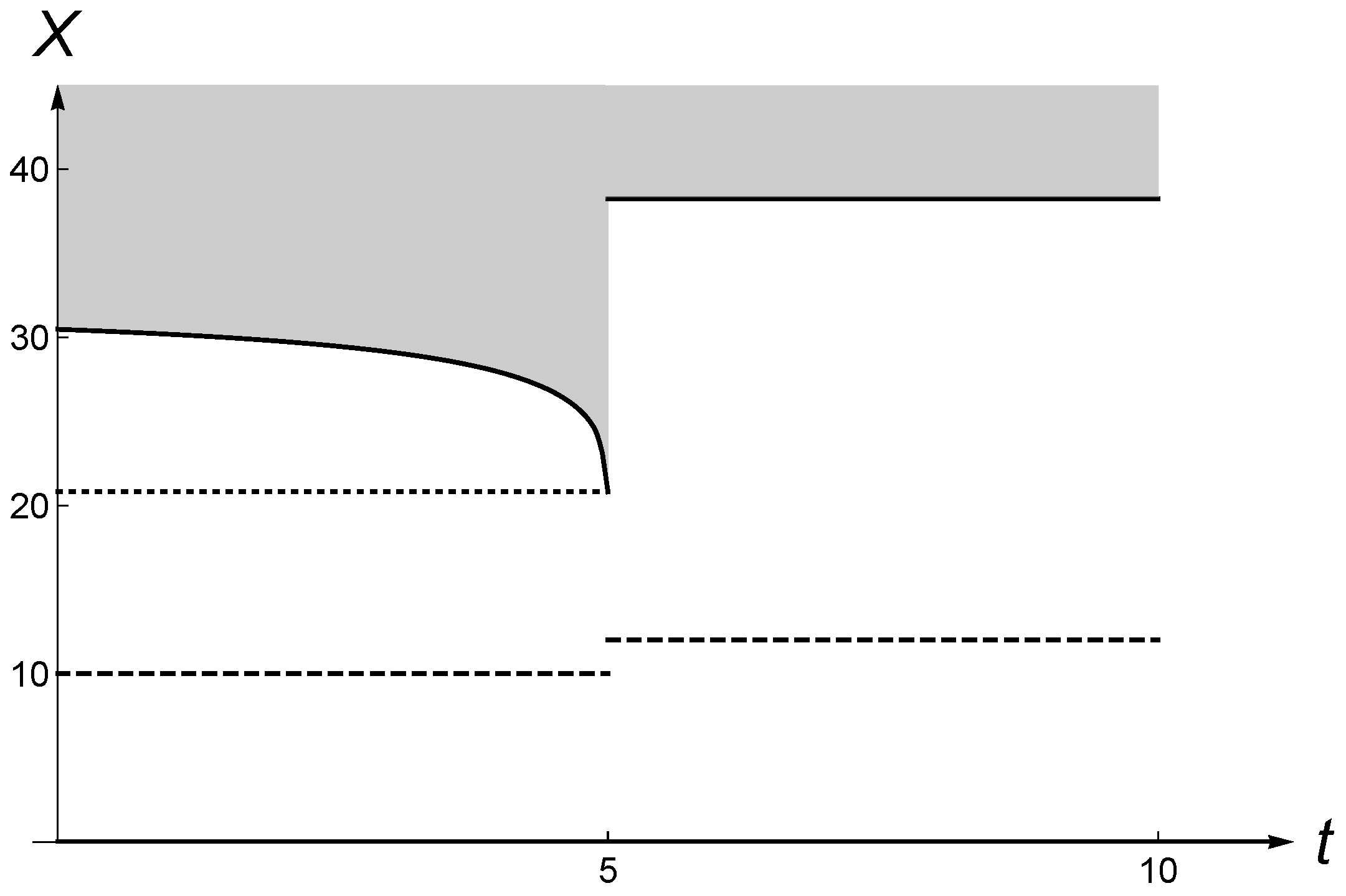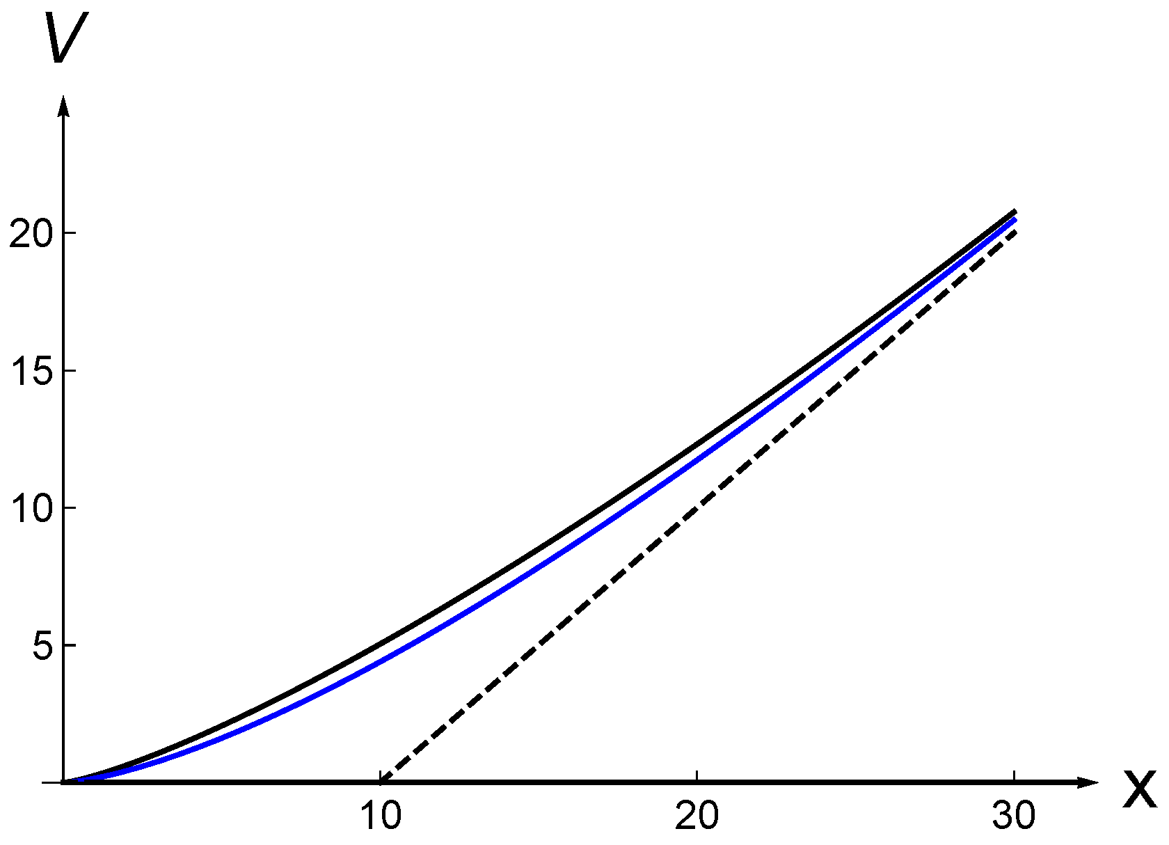Figure 1 illustrates the shape of $b_1$.

Table 1. This table compares the integral equation (IE) method to the binomial (B) tree approach for various sets of parameter values. The IE method was computed using 200, 500 and 1000 time steps. The binomial tree method was compute using 200 time steps. The true value is based on the binomial tree method with 20,000 steps.

$(\mathit{r},\mathit{\delta },\mathit{\sigma },{\mathit{K}}_1,{\mathit{K}}_2,\mathit{T})$	${\mathit{X}}_0$	IE 200	IE 500	IE 1000	B 200	True Price
(0.05,0.05,0.2,10,11,5)	7	0.9527	0.9527	0.9528	0.9528	0.9528
	8	1.2842	1.2844	1.2844	1.2844	1.2844
	9	1.6748	1.6751	1.6751	1.6752	1.6751
	10	2.1266	2.1269	2.1270	2.1269	2.1270
	11	2.6407	2.6412	2.6414	2.6414	2.6413
(0.07,0.03,0.3,10,12,5)	7	2.9421	2.9421	2.9422	2.9424	2.9422
	8	3.5093	3.5094	3.5094	3.5097	3.5094
	9	4.1017	4.1018	4.1018	4.1024	4.1018
	10	4.7177	4.7178	4.7179	4.7186	4.7179
	11	5.3559	5.3561	5.3562	5.3570	5.3562
(0.03,0.07,0.3,10,12,3)	7	0.8619	0.8620	0.8621	0.8621	0.8621
	8	1.1809	1.1811	1.1812	1.1810	1.1812
	9	1.5625	1.5629	1.5630	1.5632	1.5630
	10	2.0092	2.0097	2.0099	2.0098	2.0099
	11	2.5224	2.5231	2.5234	2.5236	2.5234

compares this integral equation (IE) method to the binomial (B) tree approach for various sets of parameter values. It shows that the IE method is accurate and convergent. Both methods are comparable in terms of CPU/RMSE (root mean squared error) tradeoff and this fact was established in the literature (see e.g. Chapter 8 in (Detemple 2006)).

3. Now we suppose that $K_1>K_2$. In this case, $\overline{V}\left(x\right)=V_2\left(x\right)$ for $x>0$. The boundary b explodes at T because the cost of waiting becomes negligible relative to the gain associated with the cost reduction. The early investment premium representation is given by

$$\begin{array}{c}V(t,x)={\mathrm{E}}_{t,x}\left[e^{-r(T-t)}{V}_2\left(X_T\right)\right]+\pi (t,x;b),\end{array}$$

(16)

$$\begin{array}{c}\pi (t,x;b)={\int }_t^T{e}^{-r(u-t)}{\mathrm{E}}_{t,x}\left[(\delta X_u-r{K}_1)I(X_u\ge b\left(u\right))\right]du,\end{array}$$

(17)

and the associated integral equation is given by

$$\begin{array}{c}\hfill b\left(t\right)-K_1={\mathrm{E}}_{t,b\left(t\right)}\left[e^{-r(T-t)}{V}_2\left(X_T\right)\right]+\pi (t,b\left(t\right);b).\end{array}$$

(18)

3. Random Jump: Direct Approach

1. In this section, we assume that the jump time $\tau$ is random and has exponential distribution with parameter $\lambda$. We assume independence of X and $\lambda$. The aim is to find the optimal investment threshold $b_1$ for the initial cost $K_1$. The solution for the future cost $K_2$ is well known and given by the value function $V_2\left(x\right)$ and threshold $b_2$

$$\begin{array}{c}{V}_2\left(x\right)=A_2{x}^{p}I(x<b_2)+(x-K_2)I(x\ge b_2),\end{array}$$

(19)

$$\begin{array}{c}{b}_2=p{K}_2/(p-1),\end{array}$$

(20)

$$\begin{array}{c}{A}_2=(b_2-K)/b_2^p,\end{array}$$

(21)

$$\begin{array}{c}p=0.5-(r-\delta )/{\sigma }^2+\sqrt{{(0.5-(r-\delta )/{\sigma }^2)}^2+2r/{\sigma }^2}.\end{array}$$

(22)

We recall that $V_2$ satisfies the smooth fit condition at $b_2$.

Now, we want to find the optimal investment strategy for an uncertain cost K that jumps at $\tau$. Clearly, the payoff has a standard call-type structure and it is optimal to invest when X is sufficiently high, i.e., when $X_t\ge b_1$ for some $b_1$. It is clear that, when $K_1>K_2$, we have that $b_1>b_2$ and that the reverse is true when $K_1<K_2$. Then, the value function V is given by

$$V\left(x\right)=\underset{b}{sup}{\mathrm{E}}_x\left[e^{-r(\tau \wedge {\tau }_b)}\left((X_{\tau \wedge {\tau }_b}-K_1)I({\tau }_b<\tau )+V_2\left(X_{\tau }\right)I({\tau }_b\ge \tau )\right)\right]$$

(23)

for $x>0$, where ${\tau }_b$ is the first hitting time of b

$${\tau }_b=inf\{t>0:X_t\ge b\}.$$

(24)

To find the optimal threshold $b_1=b_{\ast }$, first, let us fix some level b and compute the value function under the corresponding strategy

$$V(x;b)={\mathrm{E}}_x\left[e^{-r\tau \wedge {\tau }_b}\left((X_{\tau \wedge {\tau }_b}-K_1)I({\tau }_b<\tau )+V_2\left(X_{\tau }\right)I({\tau }_b\ge \tau )\right)\right],$$

(25)

which can be rewritten as

$$V(x;b)=\lambda {\int }_0^{\infty }{e}^{-\lambda T}{\mathrm{E}}_x\left[e^{-r{\tau }_b}(b-K_1)I({\tau }_b<T)+e^{-rT}{V}_2\left(X_T\right)I({\tau }_b\ge T)\right]dT$$

(26)

for $x>0$ as $\tau$ and X are independent. Let us fix T and compute the expectation

$$V_0(x;b,T):={\mathrm{E}}_x\left[e^{-r{\tau }_b}(b-K_1)I({\tau }_b<T)+e^{-rT}{V}_2\left(X_T\right)I({\tau }_b\ge T)\right]$$

(27)

for $x>0$. This can be calculated using the known distribution of $maxX$, the joint distribution of $(X_T,maxX)$ and the closed form expression for $V_2$.

Lemma 1.

(i) If $K_1>K_2$, we consider only $b>b_2$ and the following expression holds:

$$\begin{array}{l}{V}_0(x;b,T)=(b-K_1)\left({\left(\frac{x}{b}\right)}^{2\varphi /{\sigma }^2}\Phi \left(d_0(T,x,b)\right)+{\left(\frac{x}{b}\right)}^{2\alpha /{\sigma }^2}\Phi (d_0(T,x,b)+2f\sqrt{T}/\sigma )\right)\\ +x{e}^{-\delta T}\left(\Phi \left(d_1(T,x,b_2)\right)-\Phi \left(d_1(T,x,b)\right)-{\left(\frac{b}{x}\right)}^{2+2\beta /{\sigma }^2}(\Phi \left(d_2(T,x,b)\right)-\Phi \left(d_2(T,x,b^2/b_2)\right))\right)\hfill \\ -K_2{e}^{-rT}\left(\Phi \left(d_3(T,x,b_2)\right)-\Phi \left(d_3(T,x,b)\right)-{\left(\frac{b}{x}\right)}^{2\beta /{\sigma }^2}(\Phi \left(d_4(T,x,b)\right)-\Phi \left(d_4(T,x,b^2/b_2)\right))\right)\hfill \\ +A_2{x}^p{e}^{-\tilde{\delta }T}\left(1-\Phi \left(d_5(T,x,b_2)\right)-{\left(\frac{b}{x}\right)}^{2p-2\beta /{\sigma }^2}\Phi \left(d_6(T,x,b^2/b_2)\right)\right)\hfill \end{array}$$

(28)

for $b>x>0$ and $T>0$, where Φ is the standard normal cdf, $\beta =\delta -r+{\sigma }^2/2$, $f=\sqrt{{\beta }^2+2r{\sigma }^2}$, $\varphi =(\beta -f)/2$, $\alpha =(\beta +f)/2$, $\tilde{\delta }=r(1-p)+\delta p+{\sigma }^{2}p(1-p)/2$ and

$$\begin{array}{c}{d}_0(T,x,b)=(log(x/b)-fT)/\left(\sigma \sqrt{T}\right),\hfill \\ d_1(T,x,b)=(log(x/b)+(r-\delta +{\sigma }^2/2)T)/\left(\sigma \sqrt{T}\right),\hfill \\ d_2(T,x,b)=(log(x/b)-(r-\delta +{\sigma }^2/2)T)/\left(\sigma \sqrt{T}\right),\hfill \\ d_3(T,x,b)=(log(x/b)+(r-\delta -{\sigma }^2/2)T)/\left(\sigma \sqrt{T}\right),\hfill \\ d_4(T,x,b)=(log(x/b)-(r-\delta -{\sigma }^2/2)T)/\left(\sigma \sqrt{T}\right),\hfill \\ d_5(T,x,b)=(log(x/b)+(r-\delta +(p-1/2){\sigma }^2)T)/\left(\sigma \sqrt{T}\right),\hfill \\ d_6(T,x,b)=(log(x/b)-(r-\delta +(p-1/2){\sigma }^2)T)/\left(\sigma \sqrt{T}\right).\hfill \end{array}$$

(ii) If $K_1<K_2$, we consider only $b<b_2$ and the following expression holds:

$$\begin{array}{cc}\hfill V_0(x;b,T)=& (b-K_1)\left({\left(\frac{x}{b}\right)}^{2\varphi /{\sigma }^2}\Phi \left(d_0(T,x,b)\right)+{\left(\frac{x}{b}\right)}^{2\alpha /{\sigma }^2}\Phi (d_0(T,x,b)+2f\sqrt{T}/\sigma )\right)\hfill \\ & +A_2{x}^p{e}^{-\tilde{\delta }T}\left(1-{\left(\frac{b}{x}\right)}^{2p-2\beta /{\sigma }^2}\right)\hfill \end{array}$$

(29)

for $b>x>0$ and $T>0$.

Proof. 

(i) The derivation is similar to the pricing of capped or barrier type options. Taking into account that $b>b_2$, we rewrite $V_0(x;b,T)$ as

$$\begin{array}{l}{\mathrm{E}}_x\left[e^{-r{\tau }_b}(b-K_1)I({\tau }_b<T)+e^{-rT}{V}_2\left(X_T\right)I({\tau }_b\ge T)\right]\\ =(b-K_1){\mathrm{E}}_x\left[e^{-r{\tau }_b}I({\tau }_b<T)\right]+{\mathrm{E}}_x\left[e^{-rT}(X_T-K_2)I(X_T\ge b_2,M_T\le b)\right]\\ +A_2{\mathrm{E}}_x\left[e^{-rT}{X}_T^{p}I(X_T\le b_2,M_T\le b)\right],\end{array}$$

(30)

where $M_T={max}_{0\le t\le T}{X}_t$ is the maximum of X on $[0,T]$. The first expectation is well known (see, e.g., Broadie and Detemple 1995). The second term can be computed as follows:

$$\begin{array}{c}{\mathrm{E}}_x\left[e^{-rT}(X_T-K_2)I(X_T\ge b_2,M_T\le b)\right]=x{e}^{-\delta T}{\widehat{\mathrm{P}}}_x(X_T\ge b_2,M_T\le b)-K_2{e}^{-rT}{\mathrm{P}}_x(X_T\ge b_2,M_T\le b),\end{array}$$

(31)

where the measure $\widehat{\mathrm{P}}$ is defined as $d\widehat{\mathrm{P}}=exp\{-{\sigma }^{2}T/2+\sigma B_T\}d\mathrm{P}$. Both probabilities on the right-hand side are known explicitly by using the joint distribution of $(X_T,M_T)$. Now, for the third term, we have

$$\begin{array}{c}{A}_2{\mathrm{E}}_x\left[e^{-rT}{X}_T^{p}I(X_T\le b_2,M_T\le b)\right]=A_2{x}^p{e}^{-\tilde{\delta }T}\tilde{\mathrm{P}}(X_T\le b_2,M_T\le b),\end{array}$$

(32)

where we defined the measure $d\tilde{\mathrm{P}}=exp\{-p^2{\sigma }^{2}T/2+p\sigma B_T\}d\mathrm{P}$. The latter probability can be also derived as we know the dynamics of X under $\tilde{\mathrm{P}}$.

(ii) This case is even simpler. The first term is the same as in (i) above, the second expectation can be written as

$$\begin{array}{cc}\hfill {\mathrm{E}}_x\left[e^{-rT}{V}_2\left(X_T\right)I({\tau }_b\ge T)\right]& =A_2{\mathrm{E}}_x\left[e^{-rT}{X}_T^{p}I(M_T\le b)\right]\hfill \\ & =A_2{x}^p{e}^{-\tilde{\delta }T}{\tilde{\mathrm{P}}}_x(M_T\le b)=A_2{x}^p{e}^{-\tilde{\delta }T}\left(1-{\left(\frac{b}{x}\right)}^{2p-2\beta /{\sigma }^2}\right),\hfill \end{array}$$

(33)

as we assumed that $b<b_2$ and $\tilde{\mathrm{P}}$ was defined above. ☐

To find the optimal exercise boundary $b_1$, we now fix an arbitrary $X_0=x$ and maximize numerically

$$V(x;b)=\lambda {\int }_0^{\infty }{e}^{-\lambda T}{V}_0(x;b,T)dT$$

(34)

over all $b>b_2$ when $K_1>K_2$ and all $b<b_2$ when $K_1<K_2$. We note that the solution of this numerical optimization does not depend on x, i.e., for any x, we obtain the same $b_1$.

Remark 1.

Formulas (28) and (29) give the value of a capped contingent claim with automatic exercise at the cap b, liquidation payoff equal to $b-K_1$ if X reaches b before T and terminal payoff at T in the complementary event given by an American option price with strike $K_2$. These formulas generalize valuation formulas for capped options with automatic exercise at the cap in Broadie and Detemple (1995) (see Corollary 2); Rubinstein and Reiner (1991).

2. Another way to find V and b is to solve the corresponding free boundary problem (see, e.g., Carr (1998) for the case of American put option with exponentially distributed random maturity)

$$\begin{array}{c}\frac{{\sigma }^2}{2}{x}^2{V}_{xx}+(r-\delta )x{V}_x-rV=\lambda (V-V_2),x<b_1,\end{array}$$

(35)

$$\begin{array}{c}V(b_1-)=b_1-K_1,\end{array}$$

(36)

$$\begin{array}{c}{V}_x(b_1-)=1,\end{array}$$

(37)

$$\begin{array}{c}V(0+)=0,\end{array}$$

(38)

where we assumed that $K_1>K_2$. As the behavior of $V_2$ changes over subregions of the domain, we solve the ordinal differential equation (ODE) separately when $x<b_2$ (i.e., $V_2\left(x\right)=A_2{x}^p$) and $b_2<x<b_1$ (i.e., $V_2\left(x\right)=x-K_2$)

$$\begin{array}{c}V\left(x\right)=B_1{x}^{{\beta }_1}+B_2{x}^p,x<b_2,\end{array}$$

(39)

$$\begin{array}{c}V\left(x\right)=C_1{x}^{{\beta }_1}+C_2{x}^{{\beta }_2}+\frac{\lambda }{\lambda +\delta }x-\frac{\lambda K_2}{r+\lambda },b_2<x<b_1,\end{array}$$

(40)

where

$$\begin{array}{c}{B}_2=\frac{\lambda A_2}{\frac{{\sigma }^2}{2}{p}^2+(r-\delta -\frac{{\sigma }^2}{2})p-(r+\lambda ),}\end{array}$$

(41)

$$\begin{array}{c}{\beta }_1=0.5-(r-\delta )/{\sigma }^2+\sqrt{{(0.5-(r-\delta )/{\sigma }^2)}^2+2(r+\lambda )/{\sigma }^2}>0,\end{array}$$

(42)

$$\begin{array}{c}{\beta }_2=0.5-(r-\delta )/{\sigma }^2-\sqrt{{(0.5-(r-\delta )/{\sigma }^2)}^2+2(r+\lambda )/{\sigma }^2}<0,\end{array}$$

(43)

and $B_1,C_1,C_2$ are unknown constants. To find them along with the optimal threshold $b_1$, we make use of the smooth and continuous pasting conditions at $b_2$ and $b_1$

$$\begin{array}{c}{B}_1{b}_2^{{\beta }_1}+B_2{b}_2^p=C_1{b}_2^{{\beta }_1}+C_2{b}_2^{{\beta }_2}+b_2-C,\end{array}$$

(44)

$$\begin{array}{c}{B}_1{\beta }_1{b}_2^{{\beta }_1-1}+B_{2}p{b}_2^{p-1}=C_1{\beta }_1{b}_2^{{\beta }_1-1}+C_2{\beta }_2{b}_2^{{\beta }_2-1}+1,\end{array}$$

(45)

$$\begin{array}{c}{C}_1{b}_1^{{\beta }_1}+C_2{b}_1^{{\beta }_2}+b_1-C=b_1-K_1,\end{array}$$

(46)

$$\begin{array}{c}{C}_1{\beta }_1{b}_2^{{\beta }_1-1}+C_2{\beta }_2{b}_2^{{\beta }_2-1}+1=1.\end{array}$$

(47)

It can be shown that this system has a unique solution and provides $b_1$ and $V\left(x\right)$ for $x<b_1$.

Now, we consider the case $K_1<K_2$, which is in fact easier to solve. As $b_1<b_2$, we have that $V_2\left(x\right)=A_2{x}^p$ for all $x<b_1$. Therefore, the solution to ODE is given by

$$\begin{array}{c}V\left(x\right)=D_1{x}^{{\beta }_1}+D_2{x}^p\end{array}$$

(48)

in the continuation region, where $D_2=B_2$ from above. Then, to obtain $D_1$ and $b_1$, we exploit the smooth and continuous pasting conditions at $b_1$

$$\begin{array}{c}{D}_1{b}_1^{{\beta }_1}+D_2{b}_1^p=b_1-K_1,\end{array}$$

(49)

$$\begin{array}{c}{D}_1{\beta }_1{b}_1^{{\beta }_1-1}+D_{2}p{b}_1^{p-1}=1.\end{array}$$

(50)

This system has the unique solution $(D_1,b_1)$.

The solution to the free boundary problem has a simple structure, but it is less explicit than (34) to the extent that some of the coefficients, in addition to the boundary, are evaluated numerically. Nevertheless, numerical implementation is straightforward and fast.

4. Random Jump and $K_1>K_2$: EIP/DJP Representation Formulas

An alternative approach is to use Ito calculus. Let us recall that the value function V is given by

$$V\left(x\right)=\underset{b>b_1}{sup}{\mathrm{E}}_x\left[e^{-r(\tau \wedge {\tau }_b)}\left((X_{\tau \wedge {\tau }_b}-K_1)I({\tau }_b<\tau )+V_2\left(X_{\tau }\right)I({\tau }_b\ge \tau )\right)\right],$$

(51)

where ${\tau }_b$ is the first hitting time of b and τ is an exponentially distributed random variable. We know that V solves the following ODE in the continuation region

$$\frac{{\sigma }^2}{2}{x}^2{V}_{xx}+(r-\delta )x{V}_x-rV=\lambda (V-V_2)$$

(52)

for $x<b_1$. As usual, we have the smooth pasting condition at $b_1$

$$V_x(b_1-)=V_x(b_1+)=1$$

(53)

and $V\left(x\right)=x-K_1$ for $x\ge b_1$.

In Theorem 1 below, we provide two representations for the value function V. The first one takes as benchmark the strategy of waiting until the jump time tau before behaving optimally using the threshold $b_2$. The value of this suboptimal waiting strategy is

$$\begin{array}{c}{V}^w\left(x\right)={\mathrm{E}}_x\left[e^{-r\tau }{V}_2\left(X_{\tau }\right)\right]\end{array}$$

(54)

for $x>0$. By using Ito’s formula and the smooth fit condition at $b_2$, this value function can be rewritten as

$$\begin{array}{cc}\hfill V^w\left(x\right)& =V_2\left(x\right)+{\mathrm{E}}_x\left[{\int }_0^{\tau }{e}^{-rs}(r{K}_2-\delta X_s)I(X_s\ge b_2)ds\right]\hfill \\ & =V_2\left(x\right)+r{K}_2{\int }_0^{\infty }{e}^{-(r+\lambda )T}{\mathrm{P}}_x(X_T\ge b_2)dT-\delta x{\int }_0^{\infty }{e}^{-(\delta +\lambda )T}{\widehat{\mathrm{P}}}_x(X_T\ge b_2)dT,\hfill \end{array}$$

(55)

where, in the second equality, we used the distribution of τ and integration by parts. As this strategy is suboptimal, there is an early investment premium. Theorem 4.1 provides a decomposition of this premium.

The second one takes the value $V_2\left(x\right)$ as the benchmark, i.e., the investment cost is taken to be $K_2$ from time 0. As the true pre-jump cost $K_1$ is greater than $K_2$, the value function V is smaller than $V_2$. The discrepancy is a delayed jump discount, also described in the next theorem.

Theorem 1.

Given the optimal investment threshold $b_1$, the value function $V\left(x\right)$ can be represented as

$$\begin{array}{cc}\hfill V\left(x\right)=& V^w\left(x\right)+\delta x{\int }_0^{\infty }{e}^{-(\delta +\lambda )T}{\widehat{\mathrm{P}}}_x(X_T\ge b_1)dT-r{K}_1{\int }_0^{\infty }{e}^{-(r+\lambda )T}{\mathrm{P}}_x(X_T\ge b_1)dT\hfill \\ & -\lambda (K_1-K_2){\int }_0^{\infty }{e}^{-(r+\lambda )T}{\mathrm{P}}_x(X_T\ge b_1)dT\hfill \end{array}$$

(56)

for $x>0$. The difference $V\left(x\right)-V^w\left(x\right)$ is an early investment premium (EIP). Alternatively,

$$\begin{array}{cc}\hfill V\left(x\right)=& V_2\left(x\right)-\delta x{\int }_0^{\infty }{e}^{-(\delta +\lambda )T}({\widehat{\mathrm{P}}}_x(X_T\ge b_2)-{\widehat{\mathrm{P}}}_x(X_T\ge b_1))dT\hfill \\ & +r{\int }_0^{\infty }{e}^{-(r+\lambda )T}(K_2{\mathrm{P}}_x(X_T\ge b_2)-K_1{\mathrm{P}}_x(X_T\ge b_1))dT\hfill \\ & -\lambda (K_1-K_2){\int }_0^{\infty }{e}^{-(r+\lambda )T}{\mathrm{P}}_x(X_T\ge b_1)dT,\hfill \end{array}$$

(57)

where $V\left(x\right)-V_2\left(x\right)$ represents a delayed jump premium/discount (DJP). The boundary $b_1$ solves the following equation:

$$\begin{array}{cc}\hfill K_1-K_2=& \delta b_1{\int }_0^{\infty }{e}^{-(\delta +\lambda )T}({\widehat{\mathrm{P}}}_{b_1}(X_T\ge b_2)-{\widehat{\mathrm{P}}}_{b_1}(X_T\ge b_1))dT\hfill \\ & -r{\int }_0^{\infty }{e}^{-(r+\lambda )T}(K_2{\mathrm{P}}_{b_1}(X_T\ge b_2)-K_1{\mathrm{P}}_{b_1}(X_T\ge b_1))dT\hfill \\ & +\lambda (K_1-K_2){\int }_0^{\infty }{e}^{-(r+\lambda )T}{\mathrm{P}}_{b_1}(X_T\ge b_1)dT.\hfill \end{array}$$

(58)

The EIP is the difference $V\left(x\right)-V^w\left(x\right)$. Equation (56) shows that this premium is the net present value of the local net gains associated with early investment. The latter consist of instantaneous dividends $\delta X$ collected, reduced by the interest loss on the strike $r{K}_1$ and by the expected jump in the strike $\lambda \left(K_1-K_2\right)$. These gains are taken into account in the pre-jump exercise region.

The DJP is the difference $V\left(x\right)-V_2\left(x\right)$. Equation (57) shows that it corresponds to the present value of the local net losses associated with the delay in the cost jump. The latter consist of the instantaneous dividend loss on the underlying $\delta X$, the net interest saved on the cost of investment $rK$ and the expected jump in the strike $\lambda (K_1-K_2)$. The dividend loss applies when the underlying is in between the thresholds $b_2$ and $b_1$. The net interest component captures savings on the opportunity cost $K_2$ when X exceeds $b_2$, net of payments on $K_1$ when X exceeds $b_1$. As shown in Equation (60) in the proof below, the first two terms can also be repackaged as a net benefit for investing early at $K_1$ (the term $\delta X-r{K}_1$ in (60)) and a net cost for delaying exercise at $K_2$ (the term $\delta X-r{K}_2$ in (60)). The DJP is negative (i.e., it is a discount) in the case $K_1>K_2$.

Proof. 

We apply the Ito–Tanaka’s formula (with jumps) for $e^{-rt}V\left(X_t\right)$

$$\begin{array}{cc}\hfill e^{-rt}V\left(X_t\right)=& V\left(x\right)+{\int }_0^t{e}^{-rs}\left(r{K}_1-\delta X_s\right)I(X_s\ge b_1)ds\hfill \\ & -\lambda {\int }_0^t{e}^{-rs}(V_2\left(X_s\right)-V\left(X_s\right)I(X_s<b_1)ds\hfill \\ & +\lambda {\int }_0^t{e}^{-rs}(V_2\left(X_s\right)-V\left(X_s\right))ds+M_t\hfill \\ \hfill =& V\left(x\right)+{\int }_0^t{e}^{-rs}\left(r{K}_1-\delta X_s\right)I(X_s\ge b_1)ds\hfill \\ & +\lambda (K_1-K_2){\int }_0^t{e}^{-rs}I(X_s>b_1)ds+M_t\hfill \end{array}$$

(59)

for $t\le \tau$, where we used (53) and that $V_2\left(x\right)-V_1\left(x\right)=K_1-K_2$ for $x>b_1$. We also note that the local time term disappears due to the smooth fit condition at $b_1$. Now, by inserting $t=\tau$, taking the expectation on both sides, using that $V\left(X_{\tau }\right)=V_2\left(X_{\tau }\right)$ and rearranging terms, we obtain

$$\begin{array}{cc}\hfill V\left(x\right)=& {\mathrm{E}}_x\left[e^{-r\tau }{V}_2\left(X_{\tau }\right)\right]-{\mathrm{E}}_x\left[{\int }_0^{\tau }{e}^{-rs}\left(r{K}_1-\delta X_s\right)I(X_s\ge b_1)ds\right]\hfill \\ & -\lambda (K_1-K_2){\mathrm{E}}_x\left[{\int }_0^{\tau }{e}^{-rs}I(X_s>b_1)ds\right]\hfill \\ \hfill =& V_2\left(x\right)+{\mathrm{E}}_x\left[{\int }_0^{\tau }{e}^{-rs}(r{K}_2-\delta X_s)I(X_s\ge b_2)ds\right]\hfill \\ & -{\mathrm{E}}_x\left[{\int }_0^{\tau }{e}^{-rs}\left(r{K}_1-\delta X_s\right)I(X_s\ge b_1)ds\right]\hfill \\ & -\lambda (K_1-K_2){\mathrm{E}}_x\left[{\int }_0^{\tau }{e}^{-rs}I(X_s>b_1)ds\right]\hfill \\ \hfill =& V_2\left(x\right)-\delta x{\int }_0^{\infty }{e}^{-(\delta +\lambda )T}({\widehat{\mathrm{P}}}_x(X_T\ge b_2)-{\widehat{\mathrm{P}}}_x(X_T\ge b_1))dT\hfill \\ & +r{\int }_0^{\infty }{e}^{-(r+\lambda )T}(K_2{\mathrm{P}}_x(X_T\ge b_2)-K_1{\mathrm{P}}_x(X_T\ge b_1))dT\hfill \\ & -\lambda (K_1-K_2){\int }_0^{\infty }{e}^{-(r+\lambda )T}{\mathrm{P}}_x(X_T\ge b_1)dT,\hfill \end{array}$$

(60)

where we used integration by parts and the probability measure $\widehat{\mathrm{P}}$ is under the numeraire X. Then, the first equality proves (56) and the final one establishes (57).

Now, to find $b_1$, we use continuous pasting at $x=b_1$ and solve the equation

$$\begin{array}{cc}\hfill b_1-K_1=& V_2\left(b_1\right)-\delta b_1{\int }_0^{\infty }{e}^{-(\delta +\lambda )T}({\widehat{\mathrm{P}}}_{b_1}(X_T\ge b_2)-{\widehat{\mathrm{P}}}_{b_1}(X_T\ge b_1))dT\hfill \\ & +r{\int }_0^{\infty }{e}^{-(r+\lambda )T}(K_2{\mathrm{P}}_{b_1}(X_T\ge b_2)-K_1{\mathrm{P}}_{b_1}(X_T\ge b_1))dT\hfill \\ & -\lambda (K_1-K_2){\int }_0^{\infty }{e}^{-(r+\lambda )T}{\mathrm{P}}_{b_1}(X_T\ge b_1)dT.\hfill \end{array}$$

(61)

As $b_1>b_2$ and $V_2\left(x\right)=x-K_2$ for $x>b_2$, we can rewrite it as

$$\begin{array}{cc}\hfill K_1-K_2=& \delta b_1{\int }_0^{\infty }{e}^{-(\delta +\lambda )T}({\widehat{\mathrm{P}}}_{b_1}(X_T\ge b_2)-{\widehat{\mathrm{P}}}_{b_1}(X_T\ge b_1))dT\hfill \\ & -r{\int }_0^{\infty }{e}^{-(r+\lambda )T}(K_2{\mathrm{P}}_{b_1}(X_T\ge b_2)-K_1{\mathrm{P}}_{b_1}(X_T\ge b_1))dT\hfill \\ & +\lambda (K_1-K_2){\int }_0^{\infty }{e}^{-(r+\lambda )T}{\mathrm{P}}_{b_1}(X_T\ge b_1)dT.\hfill \end{array}$$

(62)

 ☐

Remark 2.

For completeness, we recall how to compute the probabilities

$$\begin{array}{c}{\widehat{\mathrm{P}}}_x(X_T\ge y)=\Phi \left(\frac{1}{\sigma \sqrt{T}}\left(log\frac{x}{y}+(r-\delta +{\sigma }^2/2)T\right)\right),\end{array}$$

(63)

$$\begin{array}{c}{\mathrm{P}}_x(X_T\ge y)=\Phi \left(\frac{1}{\sigma \sqrt{T}}\left(log\frac{x}{y}+(r-\delta -{\sigma }^2/2)T\right)\right).\end{array}$$

(64)

It is then straightforward to solve the Equation (58) numerically.

In the model with $K_1>K_2$, the cost of investment decreases at the random time τ. Potential economic applications include cases where regulations such as investment tax credits, foreign investment subsidies and preferential tax treatments matter. Countries seeking to boost employment opportunities and promote growth are often led to consider those policies in order to attract potential employers. Cities use similar incentive packages to enhance their attractiveness for new investments (e.g., the competition for Amazon’s second headquarters). In such situations, firms may be led to decide whether to invest now or wait until a potential new beneficial policy is implemented.

5. Random Jump and $K_1<K_2$: EIP/DJP Representation Formulas

In the case $K_1<K_2$, we can apply the similar arguments as in the previous section, but with slight adjustments in the calculations. It is clear that the optimal threshold $b_1$ is below $b_2$. Thus, $V_2\left(x\right)=x-K_2$ for $x>b_2$ and $V_2\left(x\right)=A_2{x}^p$ for $b_1<x<b_2$. Thus, if we apply the Ito–Tanaka formula, we obtain

$$\begin{array}{cc}\hfill e^{-rt}V\left(X_t\right)=& V\left(x\right)+{\int }_0^t{e}^{-rs}\left(r{K}_1-\delta X_s\right)I(X_s\ge b_1)ds\hfill \\ & +\lambda (K_1-K_2){\int }_0^t{e}^{-rs}I(X_s>b_2)ds\hfill \\ & +\lambda {\int }_0^t{e}^{-rs}(A_2{X}_s^p-X_s+K_1)I(b_1<X_s<b_2)ds+M_t.\hfill \end{array}$$

Then, if we employ the same arguments in the previous section, we derive the following formulas for $V\left(x\right)$ and $b_1$.

Theorem 2.

The value function $V\left(x\right)$ can be represented as

$$\begin{array}{cc}\hfill V\left(x\right)=& V_2\left(x\right)+(\delta +\lambda )x{\int }_0^{\infty }{e}^{-(\delta +\lambda )T}({\widehat{\mathrm{P}}}_x(X_T\ge b_1)-{\widehat{\mathrm{P}}}_x(X_T\ge b_2))dT\hfill \\ & -(r+\lambda ){\int }_0^{\infty }{e}^{-(r+\lambda )T}(K_1{\mathrm{P}}_x(X_T\ge b_1)-K_2{\mathrm{P}}_x(X_T\ge b_2))dT\hfill \\ & -\lambda A_2{x}^p{\int }_0^{\infty }{e}^{-(\tilde{\delta }+\lambda )T}({\tilde{\mathrm{P}}}_x(X_T\ge b_1)-{\tilde{\mathrm{P}}}_x(X_T\ge b_2))dT,\hfill \end{array}$$

(65)

and the optimal investment threshold $b_1$ solves the equation

$$\begin{array}{cc}\hfill b_1-K_1=& A_2{b}_1^p+(\delta +\lambda )b_1{\int }_0^{\infty }{e}^{-(\delta +\lambda )T}({\widehat{\mathrm{P}}}_{b_1}(X_T\ge b_1)-{\widehat{\mathrm{P}}}_{b_1}(X_T\ge b_2))dT\hfill \\ & -(r+\lambda ){\int }_0^{\infty }{e}^{-(r+\lambda )T}(K_2{\mathrm{P}}_{b_1}(X_T\ge b_1)-K_1{\mathrm{P}}_{b_1}(X_T\ge b_2))dT\hfill \\ & -\lambda A_2{b}_1^p{\int }_0^{\infty }{e}^{-(\tilde{\delta }+\lambda )T}({\tilde{\mathrm{P}}}_{b_1}(X_T\ge b_1)-{\tilde{\mathrm{P}}}_{b_1}(X_T\ge b_2))dT.\hfill \end{array}$$

(66)

The model with $K_1<K_2$ covers applications where the cost of investment can increase at a random time τ. This situation arises, in particular, when a regulator considers the removal of a subsidy that provides incentives for investments in a specific sector. The renewable power industry, which has benefitted from such incentives for many years, is a case in point. It now faces the reverse situation where regulators in many countries are considering reducing subsidies, hence increasing investment costs, due to improvements in the competitiveness of the sector. Another example is when a regulator imposes a penalty on certain types of industrial activities. Policies designed to combat climate change illustrate this case. Regulations to curb harmful emissions of fossil fuel power plants increase the cost of investments in the sector and affect the decisions of operators.

The case $K_1<K_2$ also arises in competitive settings where the opportunities of a firm are affected by the actions of a rival. For instance, a firm may be considering an investment opportunity with development cost $K_1$ if it is first to move. However, if the rival moves first, the cost jumps to $K_2>K_1$, reflecting the need to differentiate the product to be developed. The uncertainty associated with the emergence of a rival places this project in the framework of this section (In competitive settings with multiple players, both revenues and costs may be affected in the event of a rival’s move. An extension of our model to a post-jump payoff $\alpha X-K_2$, where $\alpha \in (0,1)$, can be used to model such situations.).

6. Infinitely Many Jumps: Free-Boundary Approach

In this section, we assume that the initial cost K can jump infinitely many times by the same fraction $\gamma \in (-1,\infty )$. All jump times are i.i.d. and have exponential distribution. To solve the valuation problem, let us make the following observation. At time zero, the value function is given by $V\left(x\right)$ for $X_0=x$. Then, at the time τ of the first jump, the payoff becomes

$${(x-K(1+\gamma ))}^{+}=(1+\gamma ){\left(\frac{x}{1+\gamma }-K\right)}^{+},$$

(67)

and thus the value function equals $(1+\gamma )V\left(X_{\tau }/(1+\gamma )\right)$. Therefore, $V\left(x\right)$ can be written as

$$V\left(x\right)=\underset{b>0}{sup}{\mathrm{E}}_x\left[e^{-r(\tau \wedge {\tau }_b)}\left((X_{{\tau }_b}-K)I({\tau }_b<\tau )+(1+\gamma )V\left(\frac{X_{\tau }}{1+\gamma }\right)I({\tau }_b\ge \tau )\right)\right],$$

(68)

where ${\tau }_b$ is the first hitting time of b and τ is an exponentially distributed random variable. The goal is to find the optimal threshold b and the value function V. First, we can deduce that V solves the following ODE in the continuation region

$$\frac{{\sigma }^2}{2}{x}^2{V}_{xx}+(r-\delta )x{V}_x-rV=\lambda (V-(1+\gamma )V\left(x/(1+\gamma )\right))$$

(69)

for $x<b$. As usual, we have the smooth pasting condition at the optimal b

$$V_x\left(b\right)=1,$$

(70)

and $V\left(x\right)=x-K$ for $x\ge b$.

The ordinary differential Equation (69) can be solved using the power function $x^p$ so that we obtain the equation for p

$$\frac{{\sigma }^2}{2}p(p-1)+(r-\delta )p-r=\lambda (1-{(1+\gamma )}^{-p+1})$$

(71)

for $p\in IR$. It can be shown that there are two roots, positive and negative. As $V\left(0\right)=0$, only the positive root $p_{+}>0$ is relevant. Thus,

$$V\left(x\right)=A{x}^{p_{+}}$$

(72)

for $x<b$. Using boundary conditions at b, we find that

$$\begin{array}{c}b=p_{+}K/(p_{+}-1),\end{array}$$

(73)

$$\begin{array}{c}A=(b-K)/b^{p_{+}}.\end{array}$$

(74)

The model with infinitely many downward jumps captures the case of investments in industries where technological progress steadily drives down costs. The solar panels industry provides a prominent example of this phenomenon. Indeed, the cost of US solar photovoltaic (PV) systems has experienced sustained decreases over the years, at all levels, i.e., residential, commercial and utility-scale. For Utility-Scale PV systems with One-Axis Tracker (100 MW), cost estimates have decreased from 5.44 $/W in 2010 to 4.59 in 2011, 3.15 in 2012, 2.39 in 2013, 2.15 in 2014, 1.97 in 2015, 1.54 in 2016 and 1.11 in 2017, as measured in 2017 dollars (see Fu et al. 2017). Moreover, cost decreases are associated with the (random) emergence of new technologies that have improved efficiency (In practice, the size of cost improvements varies over time depending on the technology deployed. Our model with fixed jump size can be used to approximate the true cost process and help the decision-making process of operators contemplating investments in the sector.).

7. Numerical Results

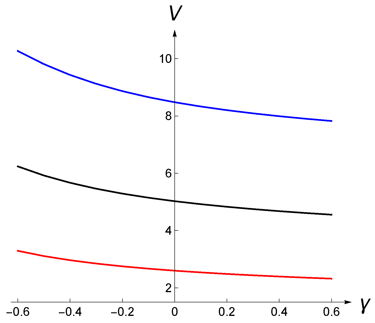
In this section, we implement the formulas described in previous sections. We choose the following central set of parameters: $r=\delta =0.03$, $\sigma =0.3$, $K_1=10$ and $K_2=K_1(1\pm \gamma )$ for $\gamma =0.2$, i.e., $K_2$ becomes in one case 8 and in the other 12. We also take $\lambda =0.2$, i.e., the jump on average occurs in five years. The figures below examine the dependence of the value function V and the investment threshold $b_1$ on the jump intensity λ and the jump size γ.

Figure 2 shows that, when $K_1>K_2$ (investment cost jumps down), the value V goes up as λ increases. This is intuitively clear as the cost K decreases sooner. In contrast when $K_1<K_2$, the value V decreases as λ increases. Figure 3 explores comparative statics w.r.t. γ or, in other words, w.r.t. $K_2$. Clearly, V is decreasing in γ. Moreover, the incremental effect of γ weakens as γ increases.

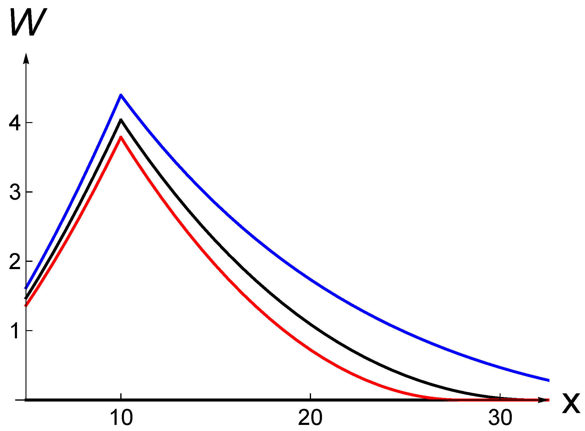
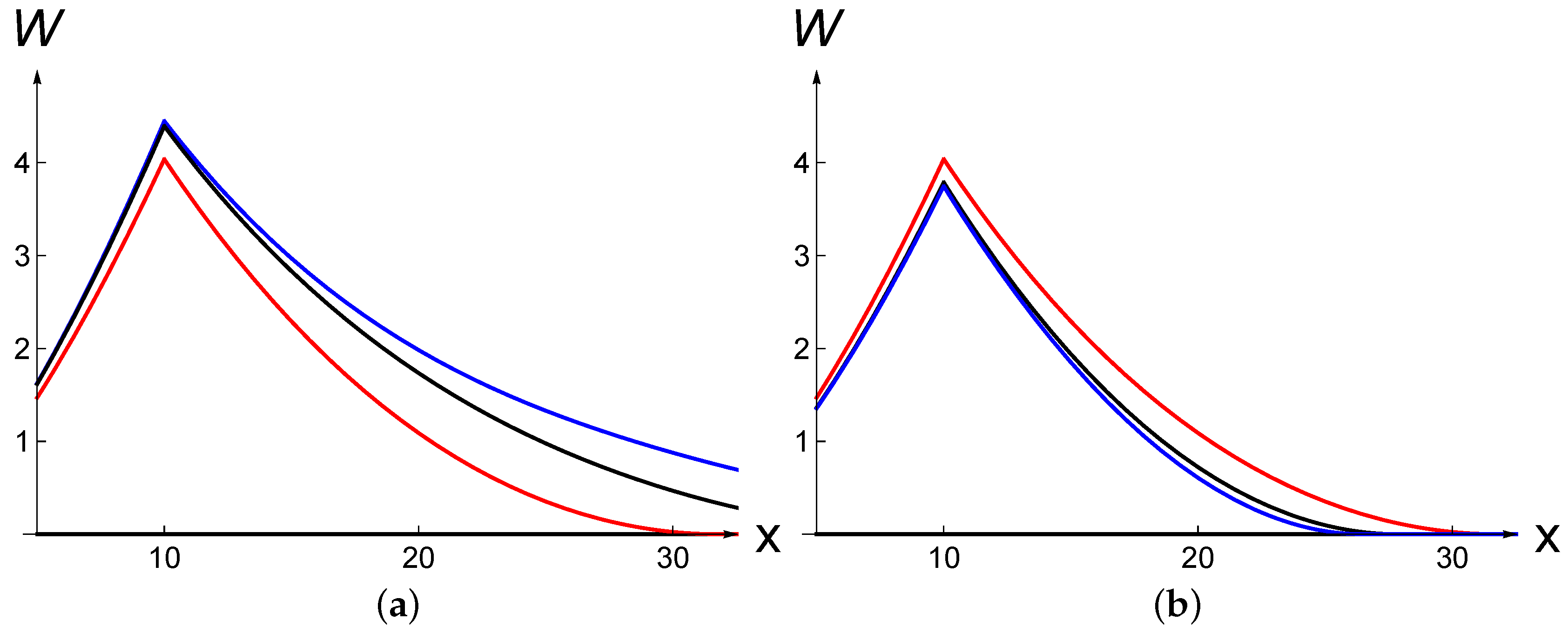
Figure 4 and Figure 5 show the value of waiting $W\left(X_0\right)\equiv V\left(X_0\right)-{(X_0-K_1)}^{+}$ as a function of x for different values of λ and γ. The general shape with respect to $X_0$ is always the same. The value of waiting increases (decreases) when $X_0$ is sufficiently low (high). This is because the value function $V\left(X_0\right)$ is strictly increasing, convex, equal to zero at $X_0=0$ (due to the GBM behavior of X) and equal to the payoff for $X_0>b_1$, and the payoff function is null for $X_0\le K_1$, then equal to $X_0-K_1$. As a result, the difference $W\left(X_0\right)$ initially increases, when the investment payoff is null, and then starts to decrease when the claim is in the money. The value of waiting always reaches a peak at $X_0=K$. Figure 4 shows that the value of waiting is a decreasing function of γ. This is because an increase in γ raises the post-jump cost of the project, which reduces the post-jump payoff. Figure 5 shows that the value of waiting is an increasing (decreasing) function of λ when γ is negative (positive). This is intuitive as a negative (positive) value of γ increases (decreases) the post-jump payoff.

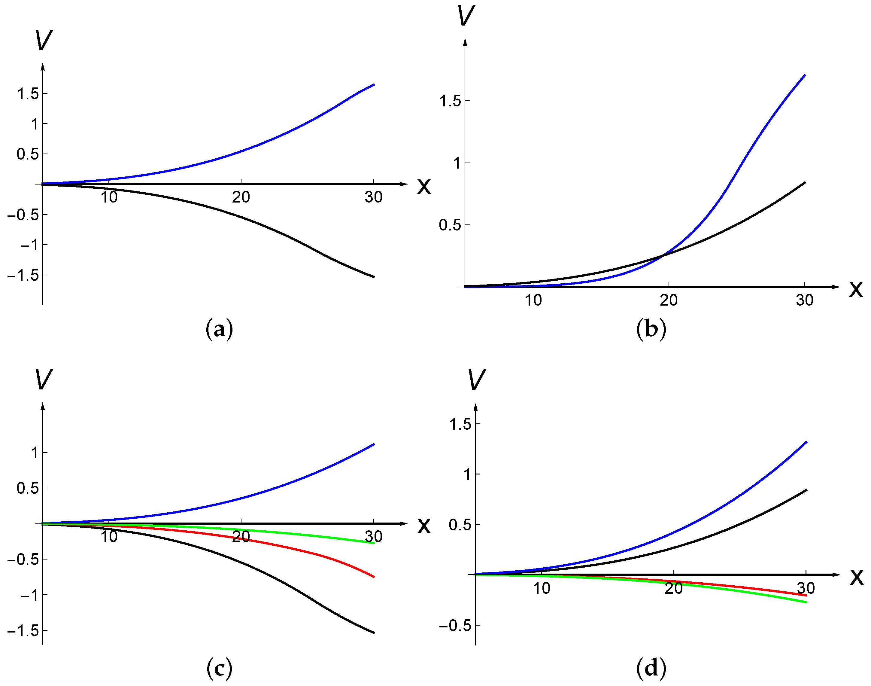
In Figure 6 (upper-left), the delayed jump premium $V-V_w$ is illustrated when $K_1<K_2$ and $K_1>K_2$. Clearly, it is positive when $K_1<K_2$ and negative in the other case. Figure 6 (upper-right) displays the early investment premium $V-V_2$. It is always non-negative because it reflects the optimality of early investment: early investment is only optimal if it creates value. The lower parts of Figure 6 illustrate the shapes of the components of DJP and EIP. The lower left panel displays the components of DJP when the post-jump cost decreases. The plot shows the positive benefit $\delta X-r{K}_1$ collected by optimally investing at $K_1$, the negative cost $\delta X-r{K}_2$ incurred by foregoing optimal investment at $K_2$ and the negative expected jump cost $\lambda (K_1-K_2)$ associated with investment at the higher $K_1$. The lower right panel shows the components of EIP when the post-jump cost decreases, namely the positive dividend component, the negative opportunity cost component and the negative expected cost jump. The sizes (absolute values) of all components in both panels are increasing functions of the underlying project value X. This is because both the likelihood of investment and the magnitudes of gains and losses increase when X increases.

Figure 7 displays the behavior of the boundary when λ and γ change. A change in the intensity of the jump process affects the optimal boundary $b_1$ but not $b_2$. This is intuitive because the boundary $b_2$ only depends on economic conditions following the jump. In contrast, a change in the size of the jump has an effect on both the pre- and post-jump boundaries. The size of the jump affects the cost of investment post-jump, hence is a determinant of the optimal investment policy.

Lastly, Figure 8 displays the case of infinitely many jumps. It focuses on the case of cost reductions by a constant fraction gamma at each jump time. The plot shows that the incremental effect, beyond the first reduction, is small. This follows because cost reductions beyond the first one occur at later dates, hence carry heavier discounts and have decreasing magnitudes.

8. Conclusions

This paper has examined the valuation of real option when the cost of investment jumps at a random time. Explicit valuation formulas, which identify and decompose the sources of value, were derived. Numerical results were provided to illustrate the behaviors of the value function, the EIP/DJP components and the optimal investment boundaries.

The methodologies developed in this paper can be used to study more general claims arising in real options applications when cost uncertainty takes the form of jumps. Projects with shutdown and restart options, abandonment options and expansion options are natural candidates for generalizations. More complex multi-stage claims, such as those involving exclusive opportunities, are also of interest in this context.