Lambda Value at Risk and Regulatory Capital: A Dynamic Approach to Tail Risk

Abstract

This paper presents the first methodological proposal of estimation of the $\mathsf{\Lambda }VaR$. Our approach is dynamic and calibrated to market extreme scenarios, incorporating the need of regulators and financial institutions in more sensitive risk measures. We also propose a simple backtesting methodology by extending the $VaR$ hypothesis-testing framework. Hence, we test our $\mathsf{\Lambda }VaR$ proposals under extreme downward scenarios of the financial crisis and different assumptions on the profit and loss distribution. The findings show that our $\mathsf{\Lambda }VaR$ estimations are able to capture the tail risk and react to market fluctuations significantly faster than the $VaR$ and expected shortfall. The backtesting exercise displays a higher level of accuracy for our $\mathsf{\Lambda }VaR$ estimations.

1. Introduction

The global financial crisis has made risk measurement and its backtesting a primary concern for regulators and financial institutions. Over the past two decades, the value at risk ($VaR$) has become the most popular method to assess the risk exposure of financial investments. One of the reasons for its widespread use is that the Basel Committee on Banking Supervision (1996a) has suggested that banks use an internal $VaR$ model for the calculation of their regulatory capital. Thus, authorities around the world have endorsed $VaR$ as the best practice or as a regulatory standard.

Despite its popularity, $VaR$ has been extensively criticized by academics. For instance, Artzner et al. (1997, 1999) have underlined some of the theoretical shortcomings of $VaR$ as a risk measure. Specifically, $VaR$ might penalize diversification since it is not subadditive and does not capture the tail risk. This is so because it does not consider losses greater than the $VaR$ amount. In addition, the recent global financial crisis has highlighted the lack of sensitivity of the $VaR$. Financial risk managers have addressed the difficulty of a rapid adjustment of its confidence levels. As a consequence, $VaR$ may lead to under-forecasting of risk estimates before the crisis or even over-forecasting of them post-crisis.

Therefore, both regulators and financial institutions have recently increased their interest in more sensitive risk measures and their backtesting. In particular, the Minimum Capital Requirements for Market Risk by the Basel Committee (2016) has proposed to move to the expected shortfall ($ES$), known also as conditional value at risk ($CVaR$), which was introduced by Artzner et al. (1997). This measure of risk, which is defined as the expected value of losses exceeding $VaR$, can solve some of the issues with the $VaR$ and has sounder theoretical properties (i.e., it fulfills subadditivity). However, many studies have pointed out the challenges of delivering a robust forecasting and backtesting of the $ES$ (see Gneiting 2011; Embrechts and Hofert 2014). Additional concerns about the $ES$ backtesting are expressed by the Basel Committee (2016), which requires that the backtesting regulatory framework will still be based on $VaR$.

In a recent paper by Frittelli et al. (2014), a new risk measure is proposed: the lambda value at risk (lambdaVaR or $\mathsf{\Lambda }VaR$) as a generalization of the $VaR$. The novelty of the $\mathsf{\Lambda }VaR$ is considering a function $\mathsf{\Lambda }$ that depends on the profits and losses (P&Ls) of the risk factors, instead of a constant confidence level $\lambda$. For how it is built, the $\mathsf{\Lambda }VaR$ assigns more risk to heavy-tailed P&L distributions and less in the opposite case. Thus, the $\mathsf{\Lambda }VaR$ should be able to discriminate the risk among assets with the same $VaR$ at level $\lambda$ but different tail behaviour of the P&L distribution. However, in this theoretical paper, there is no explanation of how the $\mathsf{\Lambda }VaR$ should be computed. The function $\mathsf{\Lambda }$ can be either increasing or decreasing, but the authors do not propose any particular shape of the $\mathsf{\Lambda }$ function or a method for its estimation.

The objective of this study is twofold: first, to provide a methodological proposal of estimation for the $\mathsf{\Lambda }VaR$ and, second, to test its effectiveness as a regulatory alternative to $VaR$. Our methodological approach makes the $\mathsf{\Lambda }VaR$ able to incorporate the actual market conditions, allowing for the reservation of more capital in crisis periods and less in normal market situations. We base the computation of the $\mathsf{\Lambda }$ function on order statistics of the historical distribution function of some selected market benchmarks. The parameters are recalculated for each out-of-sample period, allowing the $\mathsf{\Lambda }VaR$ to capture the market changes and assess the different reactivity of the assets to the market variations. Thus, our $\mathsf{\Lambda }VaR$ estimations are able to discriminate the risk among assets with different tail behaviour in respect to the market. In addition, the $\mathsf{\Lambda }VaR$ can be specified differently according the particular risk profile. We call this method of estimation, ‘dynamic benchmark approach’. We also propose a simple backtesting methodology by extending the $VaR$ hypothesis-testing framework by Kupiec (1995) to the $\mathsf{\Lambda }VaR$ in order to have an initial evaluation of the $\mathsf{\Lambda }VaR$ accuracy1.

We test our $\mathsf{\Lambda }VaR$ effectiveness as a regulatory alternative to $VaR$ under extreme downward scenarios of the financial crisis and different assumptions on the P&L distribution. We compare these estimates with those of the $VaR$ and the $ES$, highlighting the different levels of reactivity to bad changes in financial markets. Hence, we perform a backtesting exercise where we compare $VaR$ and $\mathsf{\Lambda }VaR$ estimations’ accuracy.

The remainder of the paper is organized as follows. Section 2 describes the new risk measure, the $\mathsf{\Lambda }VaR$, from a theoretical point of view, and our proposal of estimation. Here, the backtesting methodology is also illustrated. Section 3 shows the results of the empirical test, consisting in the computation, backtesting, and comparison of the risk measures. Section 4 concludes.

2. Method

2.1. Current Risk Measures and $\mathsf{\Lambda }VaR$

Because of its simple formulation and interpretation, the $VaR$ is the most popular tool for measuring financial risk. Let X be the random variable that models asset returns (i.e., profit and loss, P&L) and $F\left(x\right)=P(X\le x)$ its cumulative distribution function. We denote by $\mathcal{P}$ the set of all the distributions. The $VaR$ of a financial asset at the confidence level $\lambda$, where $0<\lambda <1$, is defined as the $\lambda$-right quantile of its P&L distribution over a certain holding period. Formally,

$$Va{R}_{\lambda }\left(X\right)=-sup\left\{x:F\left(x\right)\le \lambda \right\}.$$

(1)

In other words, $Va{R}_{\lambda }$ represents the maximum loss x that may occur such that the probability of losing more than the amount x is lower than $\lambda$ over a certain time horizon. The main advantage of the $VaR$ is that a single number immediately provides the idea of the amount of capital that should be allocated to cover the risk of a financial asset. On the other hand, the $VaR$ has many critics. Academics have pointed out that $VaR$ might penalize diversification because of its lack of subadditivity; that is, the risk of the portfolio in terms of the $VaR$ may be larger than the sum of the risks of its components. In addition, practitioners have noticed its lack of sensitivity, especially during changes in the economic cycle. It seems to be difficult to rapidly decrease the confidence level when a crisis period occurs and to increase it post-crisis. Moreover, the $VaR$ does not allow practitioners to discriminate the risk of financial positions having the same $\lambda$-right quantile but a different tail thickness, thereby failing to capture extreme events.

The experiences from the global financial crisis have raised additional doubts about the accuracy of internal $VaR$ models. These serious concerns have prompted the recent response by the Basel Committee (2016) to move to another risk measure known as the expected shortfall ($ES$), which was introduced by Artzner et al. (1997). Formally, the ES of an asset X at confidence level $\lambda$, where $0<\lambda <1$, is given by

$$E{S}_{\lambda }\left(X\right)=E[-X|X\le -Va{R}_{\lambda }\left(X\right)]=\frac{{\int }_0^{\lambda }Va{R}_s\left(X\right)ds}{\lambda }.$$

(2)

By definition, this risk measure is able to capture the tail risk. In addition, it does not discourage diversification since it satisfies the subadditivity property. However, several studies have found that the most significant issue associated with the $ES$ is the difficulty of achieving robust estimation and backtesting (see Gneiting 2011; Embrechts and Hofert 2014).

The new risk measure introduced by Frittelli et al. (2014), the $\mathsf{\Lambda }VaR$, may be a valid alternative. The $\mathsf{\Lambda }VaR$ is a generalization of the $VaR$ and is based on the fact that the confidence level can change and adjust according to the risk factor P&L.

Specifically, it considers a function $\mathsf{\Lambda }$ instead of a constant confidence level $\lambda$. Formally, given a monotone and right continuous function $\mathsf{\Lambda }:\mathbb{R}\to \left[{\lambda }_m,{\lambda }_M\right]$ with $0<{\lambda }_m\le {\lambda }_M<1$, the $\mathsf{\Lambda }VaR$ of the asset return X is a generalized quantile represented by the map $\mathsf{\Lambda }VaR:\mathcal{P}\to \mathbb{R}$ defined as follows:

$$\mathsf{\Lambda }VaR\left(F\right):=-sup\left\{m\in \mathbb{R}\mid F\left(x\right)\le \mathsf{\Lambda }\left(x\right),\forall x\le m\right\}.$$

(3)

Intuitively, the $\mathsf{\Lambda }VaR$ of the financial position X is given by the smallest intersection between F and $\mathsf{\Lambda }$ if both are continuous. The function $\mathsf{\Lambda }$ plays a key role in the definition of the $\mathsf{\Lambda }VaR$ and adds flexibility. From a theoretical point of view, no particular properties are required by $\mathsf{\Lambda }$, which can be either increasing or decreasing. In addition, $\mathsf{\Lambda }VaR$ satisfies the mathematical properties of interest from a risk management point of view (Burzoni et al. 2017; Frittelli et al. 2014).

In Section 2.2, we propose a methodology to compute the $\mathsf{\Lambda }VaR$, and we explain our $\mathsf{\Lambda }$ choices, the assumptions behind them, and the empirical implications. See Figure 1 for a clearer understanding of this.

2.2. The Proposal of $\mathsf{\Lambda }VaR$ Estimation: A Dynamic Benchmark Approach

This section contains a guide to the estimation of the $\mathsf{\Lambda }VaR$ and our methodological proposal. As discussed in Section 2.1, the flexibility of the $\mathsf{\Lambda }VaR$ stems from the possibility of choosing the function $\mathsf{\Lambda }$ instead of fixing a confidence level $\lambda$. From a theoretical point of view, $\mathsf{\Lambda }$ is a right continuous function taking values on the interval $\left[{\lambda }_m,{\lambda }_M\right]$ with $0<{\lambda }_m\le {\lambda }_M<1$. No additional constrictions are required on this function, which can be either increasing or decreasing.

The estimation of the $\mathsf{\Lambda }VaR$ consists in four main steps: 1. fixing the $\mathsf{\Lambda }$ range of values, $\left[{\lambda }_m,{\lambda }_M\right]$; 2. deciding the $\mathsf{\Lambda }$ direction (increasing or decreasing); 3. choosing the $\mathsf{\Lambda }$ functional shape; 4. estimating the $\mathsf{\Lambda }$ parameters.

Concerning the choice of the $\mathsf{\Lambda }$ range of values, we first fix the minimum ${\lambda }_m$ close to 0, specifically 0.001; we have proved, computationally, that a further reduction of ${\lambda }_m$ would determine an increase in the capital requirement without any benefit in terms of reduction in the number of violations. However, the main issue is the choice of the maximum, ${\lambda }_M$, that we call the $\mathsf{\Lambda }VaR$ confidence level. This choice reflects the bank risk aversion profile. Common opinion and empirical evidence have shown a level of doubt about high confidence levels for the $VaR$. In addition, the Basel Committee has recently proposed the calibration of new risk measures for extreme scenarios. This might suggest considering a confidence level below $1\%$. Hence, our first choice is ${\lambda }_M$ equal to $1\%$, defining $1\%$ $\mathsf{\Lambda }VaR$. However, from a managerial point of view, banks may consider the use of new risk measures that release capital in the case of higher confidence levels. For this reason, in Section 3, we also examined a $\mathsf{\Lambda }VaR$ with ${\lambda }_M$ values equal to $1.5\%$ and $2\%$.

Regarding the second step, we suggest that the decision on the $\mathsf{\Lambda }$ direction should be taken according to the expectation about the economic cycle. In the case of a bearish market trend, increasing function $\mathsf{\Lambda }$ should make it easier to detect downside scenarios and reduce the number of overdrafts between the realized P&L and the $\mathsf{\Lambda }VaR$ estimations. On the other hand, a decreasing $\mathsf{\Lambda }$ may be more convenient in periods of expected growth, allowing for a reduction in the capital aside, which may boost the investments.

The third step consists in examining different functional forms of continuous $\mathsf{\Lambda }$. In the increasing case, it turns out to be an immediate and, at the same time, sensible specification to have a $\mathsf{\Lambda }$ function that is obtained by linear interpolation. Formally, we divide the real line of the P&L and probabilities in $n+1$ intervals, where n is the number of data points used for the interpolation. Let us denote with ${\pi }_i$ and ${\lambda }_i$, where $i=1,2,\dots n$, the extremes of the interpolating intervals on the P&L and probability axis, respectively. For any P&L amount $x<{\pi }_1$, we fix $\mathsf{\Lambda }\left(x\right)={\lambda }_1={\lambda }_m$, for $x\ge {\pi }_n$ we fix $\mathsf{\Lambda }\left(x\right)={\lambda }_n={\lambda }_M$, and when ${\pi }_1\le x<{\pi }_n$ we suggest that

$$\mathsf{\Lambda }\left(x\right)=\sum _{i=1}^{n-1}{\mathbf{1}}_{\left[{\pi }_i,{\pi }_{i+1}\right)}\left((x-{\pi }_i){\displaystyle \frac{{\lambda }_{i+1}-{\lambda }_i}{{\pi }_{i+1}-{\pi }_i}}+{\lambda }_i\right).$$

(4)

In the decreasing case, for $x<{\pi }_1$, we fix $\mathsf{\Lambda }\left(x\right)={\lambda }_M$, for $x\ge {\pi }_n$ we fix $\mathsf{\Lambda }\left(x\right)={\lambda }_m$, and when ${\pi }_1\le x<{\pi }_n$ we fix $\mathsf{\Lambda }$ as follows:

$$\mathsf{\Lambda }\left(x\right)=\sum _{i=1}^{n-1}{\mathbf{1}}_{\left[{\pi }_i,{\pi }_{i+1}\right)}\left((x-{\pi }_i){\displaystyle \frac{{\lambda }_{n-i}-{\lambda }_{n-i+1}}{{\pi }_{i+1}-{\pi }_i}}+{\lambda }_{n-i+1}\right).$$

(5)

The final step of the $\mathsf{\Lambda }$ calibration consists of the estimation of ${\lambda }_i$ and ${\pi }_i$. Here, the financial manager’s aversion or propensity towards the risk plays a crucial role. In the increasing case, more $\mathsf{\Lambda }$ is shifted on the right of the P&L axis, the $\mathsf{\Lambda }VaR$ absolute value is larger, and the capital allocated as risk protection is thus larger. In the decreasing case, the situation is reversed; financial managers adopting a prudential approach may choose $\mathsf{\Lambda }$ to be more translated on the left. These considerations have a direct impact on the choice of the points ${\pi }_i$. In particular, if the objective is to strengthen the capital requirement, the points ${\pi }_i$ will be arranged on the right, in the increasing case, or on the left, in the decreasing case; on the contrary, if the objective is to release capital, the points ${\pi }_i$ will be arranged more on the left, in the increasing case, or on the right, in the decreasing case.

First, we fix the points ${\lambda }_i$, adopting a neutral approach. With the exception of ${\lambda }_1$ and ${\lambda }_n$, which are fixed equal to the minimum (${\lambda }_m=0.001$) and maximum (${\lambda }_M=0.01$) $\mathsf{\Lambda }$ value, respectively, the other ${\lambda }_i$ values are determined by an equipartition of the interval $(0,{\lambda }_M]$, specifically ${\lambda }_i={\lambda }_M/(n-1)\times (i-1)$ with $i=2,\dots ,n-1$. On the other hand, another scale that thickens the points close to the maximum ${\lambda }_M$ (or the minimum ${\lambda }_m$) would determine an increase (or decrease) of the concavity of the $\mathsf{\Lambda }$ function between ${\pi }_1$ and ${\pi }_n$, and this would have an impact on the capital requirement depending on the $\mathsf{\Lambda }$ direction. One could choose to modify the capital requirement by varying either the vertical coordinates (on the probability axis) or the horizontal coordinates (on the P&L axis) of the $\mathsf{\Lambda }$ function or even both. We prefer to maintain a neutral approach on the vertical coordinates of $\mathsf{\Lambda }$ and provide different $\mathsf{\Lambda }VaR$ specifications by varying only the horizontal coordinates as described in the paragraph below. However, there are no restrictions on this point and other solutions can be experimented, although the number of ad hoc choices on the model should remain limited.

Finally, we estimate the points ${\pi }_i$ using the following approach, which we call dynamic benchmark approach. We calibrate $\mathsf{\Lambda }$ on the statistics of the tail historical distribution of selected benchmarks. The idea is to compare the tails of an asset P&L distribution with a function $\mathsf{\Lambda }$ that directly depends on the tails of the market historical distribution. In such a way, we make the capital requirement decision depend on the behaviour of the risk factor returns in comparison with market returns. With this choice, we expect that the $\mathsf{\Lambda }VaR$ is able to incorporate the recent market changes and the particular asset reactions faster than other risk measures. This approach is dynamic since the $\mathsf{\Lambda }$ function is continuously recalculated by using the same rolling window of the risk measure and maintained constant throughout the out-of-sample period. However, the $\mathsf{\Lambda }$ function must be unique for each risk factor, so the calibration cannot depend on specific features of the assets under analysis.

We set the points ${\pi }_i$ on the basis of the n order statistics of the benchmark historical P&L distributions. We propose taking four points ${\pi }_i$, so $n=4$. In our opinion, this number of points represents a good trade-off between fitting accuracy and function parametric complexity. However, this choice does not substantially affect the results. We fix ${\pi }_1$ equal to the smallest order statistic; that is, the minimum of all the benchmark returns, ${\pi }_1=min(r_{min1},\dots r_{minj},\dots r_{minB})$, where $r_{minj}$ is the minimum return of the j-th benchmark, and B is the total number of benchmarks. We fix ${\pi }_2$, ${\pi }_3$, and ${\pi }_4$ equal to the maximum, mean, and minimum of their historical $\lambda \%$-$VaR$, respectively. The choice of the confidence level $\lambda$ for the benchmarks’ $VaR$ depends on the risk aversion profile. In the case of an increasing $\mathsf{\Lambda }$, a $5\%$-$VaR$ represents a more prudential choice than a $1\%$-$VaR$, since $5\%$-$VaR$ order statistics shift the $\mathsf{\Lambda }$ function more to the right. The converse holds in the case of a decreasing $\mathsf{\Lambda }$. The rolling window used for computing the 1–$5\%$-$VaR$ of the benchmarks should be the same used for computing the $VaR$ and $\mathsf{\Lambda }VaR$ of the risk factors.

For instance, if we test the $\mathsf{\Lambda }VaR$ on equity markets, good benchmark candidates are the equity indexes that have the highest volume of transactions and that represent the markets in which the bank’s trading activity is concentrated. In our empirical test, we selected the S&P500 (US), the FTSE 100 (UK), and the EURO STOXX 50 (Eurozone). Alternatively, the selection of these benchmarks as well as the interval of confidence for their $VaR$ computation can be done externally by the regulator. Figure 1 shows two examples of the $\mathsf{\Lambda }VaR$ estimations for the increasing and decreasing cases.

In conclusion, more advanced and sophisticated $\mathsf{\Lambda }$ estimations may be considered provided that the mathematical properties of the $\mathsf{\Lambda }VaR$ are preserved. However, increasing the $\mathsf{\Lambda }$ complexity is not consistent with the purpose of this study. Our benchmark approach is easy to compute and allows for a better understanding of the new risk measure.

2.3. Backtesting Method

The reliability and accuracy of a risk measure depend on its ability to predict and cover future unexpected losses. For this reason, the risk measure should be backtested with appropriate methods. According to the Basel Committee on Banking Supervision (1996b), the backtesting, that is, the statistical procedure of comparing realized profits and losses y with forecast risk measures x, is essential in the validation process of risk management internal models (see Jorion 2007).

The Basel Committee on Banking Supervision (1996b) has set up a regulatory backtesting framework for internal $VaR$ models in order to monitor the frequency of exceptions; this is known as the traffic light approach. This procedure is carried out by comparing the last 250 daily 1% $VaR$ estimates with the corresponding daily P&L outcomes. The accuracy of the model is then evaluated by counting the number of exceptions during this period. Many alternative proposals have been introduced in the literature for $VaR$ (see Campbell 2005; Christoffersen 2010; Berkowitz et al. 2011 for a detailed review). On the other hand, the backtesting of $\mathsf{\Lambda }VaR$ has been studied only recently by Corbetta and Peri (2017).

In this paper, we propose using, for the backtesting of the risk measures, the unilateral hypothesis test by Kupiec (1995), which is the first $VaR$ method introduced in the literature and is the most widely known and used. This is also one of the simplest tests in that it allows for an intuitive interpretation and comparison of the $VaR$ and $\mathsf{\Lambda }VaR$ backtesting performances. Kupiec’s test, known as unconditional coverage (UC) or portion of failure (POF) test, measures whether the number n of exceptions $y<x$ over a specific number of observations N in the backtesting window is consistent with the confidence level $\lambda$. The $VaR$ model should be accepted if the frequency of exceptions over the specific time interval, $\widehat{\lambda }$, does not significantly differ from the confidence level, $\lambda$. Hence, the null and the alternative hypothesis for the POF test are given by

$$H_0:\lambda =\widehat{\lambda }=\frac{n}{N},H_1:\widehat{\lambda }>\lambda .$$

(6)

Under $H_0$, where the $VaR$ is considered to be ‘correct’, the number of exceptions over the selected time period follows a binomial distribution. Thus, the POF test is conducted with the following log-likelihood ratio:

$$L{R}_{POF}=-2ln\left(\frac{{(1-\lambda )}^{N-n}{\lambda }^n}{{(1-\left(\frac{n}{N}\right))}^{N-n}{\left(\frac{n}{N}\right)}^n}\right)\sim {\chi }_1^2.$$

(7)

Asymptotically, as the number of observations N goes to infinity, the test will be distributed as a ${\chi }^2$ with 1 degree of freedom. If the $L{R}_{POF}$ statistic exceeds the critical value of the ${\chi }_1^2$, the model should be rejected. This critical level depends on the test confidence level. However, the choice of the confidence level is based on the balance of two types of errors: a type I error to reject a correct model and a type II error to accept an incorrect model. Increasing the significance level implies larger type I errors but smaller type II errors, and vice versa. Best practice suggests the use of a confidence level at least equal to 5% to control the type II errors, which can be very costly.

We extend the $VaR$ backtesting framework to the $\mathsf{\Lambda }VaR$ while maintaining the same structure and fundamental meaning. Being a generalized quantile, the confidence level of the $\mathsf{\Lambda }VaR$ changes according to the $\mathsf{\Lambda }$ function. A good candidate for the $\mathsf{\Lambda }VaR$ confidence level is the maximum of the $\mathsf{\Lambda }$ function, $max\left(\mathsf{\Lambda }\right)$. Hence, we propose adjusting the POF test by considering the $max\left(\mathsf{\Lambda }\right)$, under the null hypothesis, instead of $\lambda$. In particular, the null and the alternative hypothesis for the $\mathsf{\Lambda }VaR$ test become

$$H_0:\frac{n}{N}\le max\left(\mathsf{\Lambda }\right),H_1:\frac{n}{N}>max\left(\mathsf{\Lambda }\right).$$

(8)

This is still an unilateral hypothesis test with the same critical region as the $VaR$ test (see Casella and Berger 2002). Hence, it can be conducted by using the same log-likelihood ratio and critical value of the $VaR$ test. The risk model is validated if the relative number of the exceptions does not exceed the target level of exceptions given by $max\left(\mathsf{\Lambda }\right)$. This adjustment provides information about the $\mathsf{\Lambda }VaR$’s accuracy and an immediate interpretation. Indeed, it verifies whether the coverage objective given by the $\mathsf{\Lambda }$ maximum has been reached. However, it has some limitations, which have been highlighted by Corbetta and Peri (2017) in their literature review. Here, we prescind from providing a complete framework on the backtesting of the $\mathsf{\Lambda }VaR$.

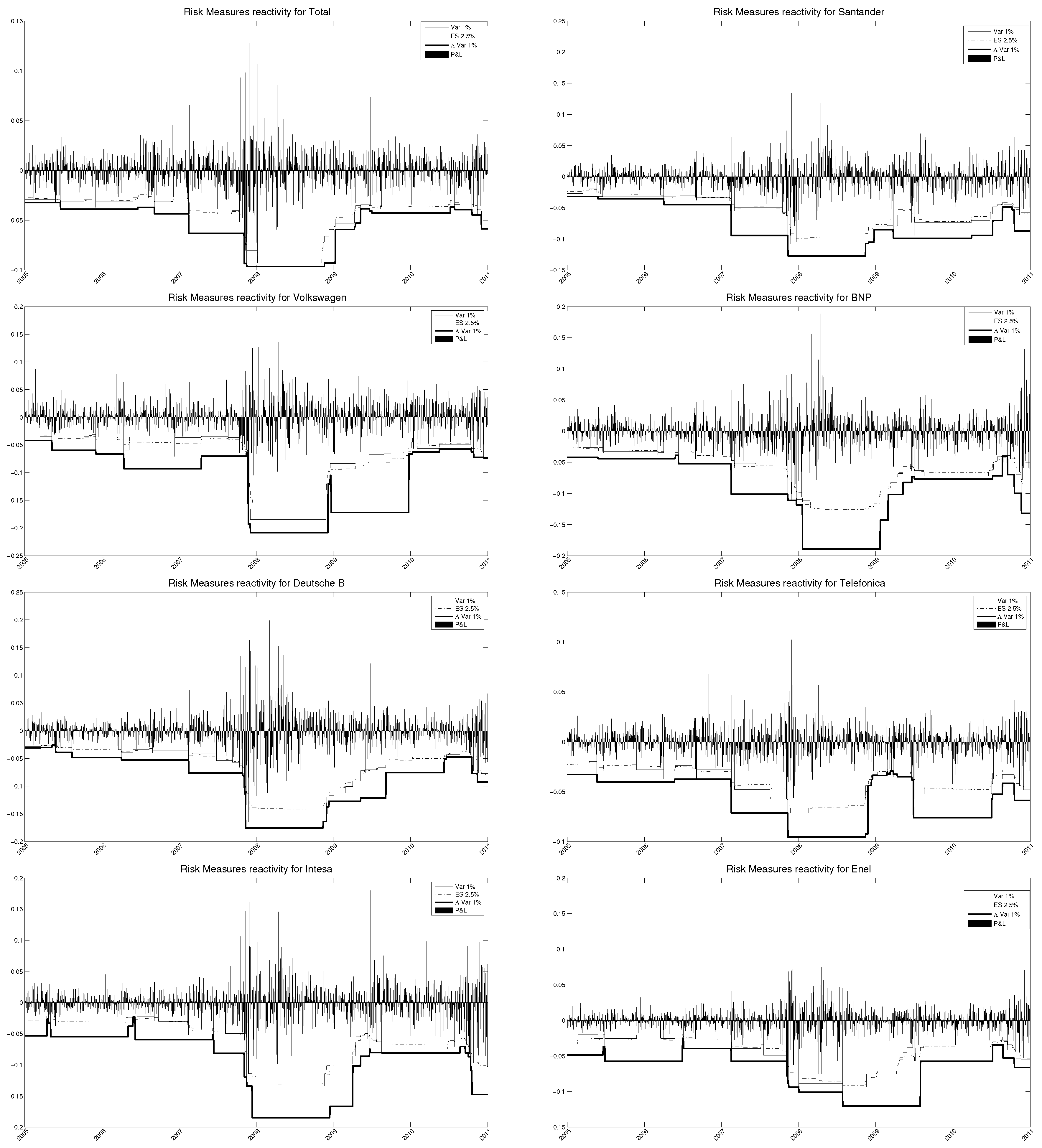
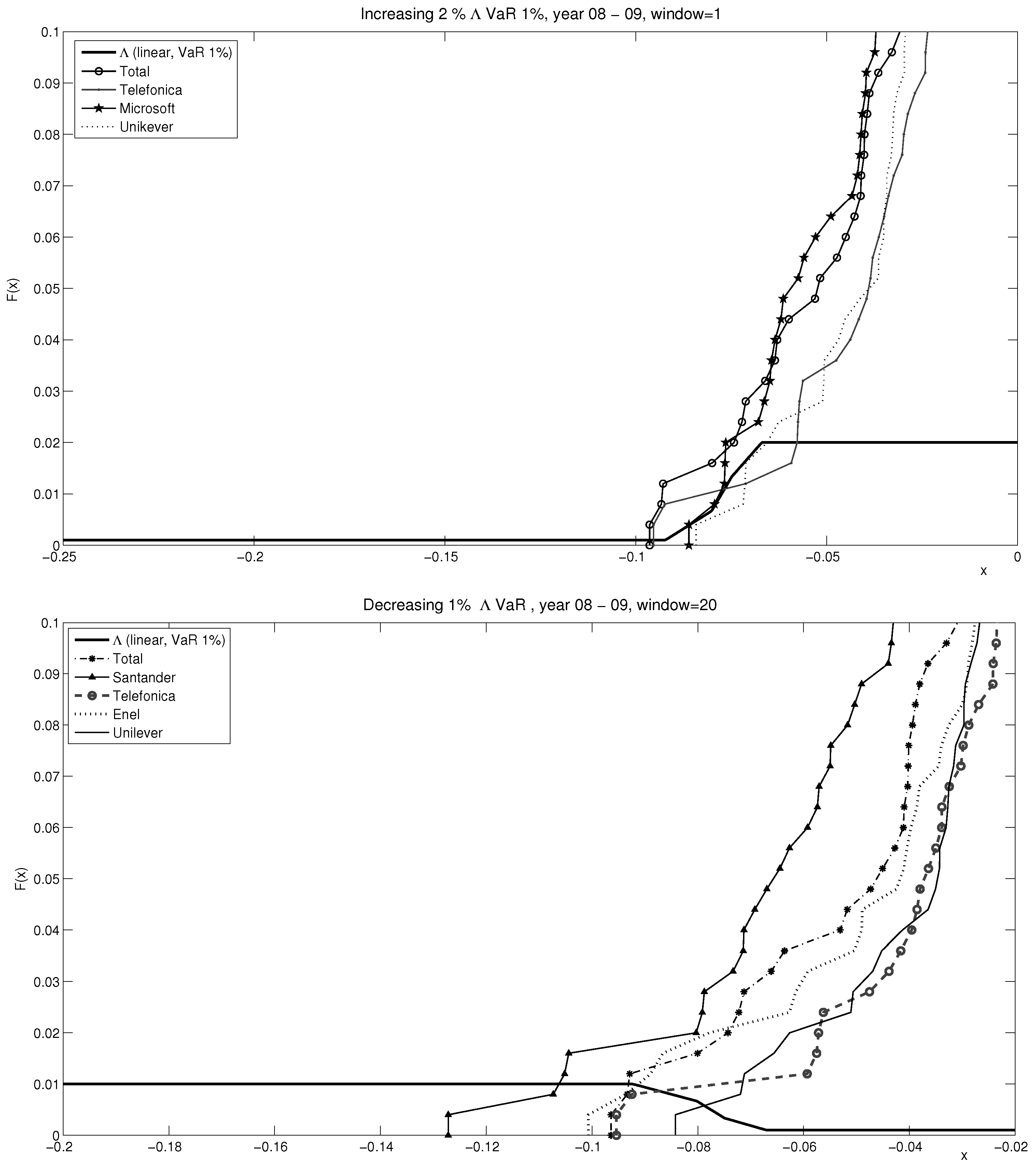
3. Empirical Analysis

In this section, we test our methodology to compute the $\mathsf{\Lambda }VaR$, the so-called dynamic benchmark approach, proposed in Section 2.2. We examine the different $\mathsf{\Lambda }VaR$ specifications and their implementation under different assumptions of the P&L distribution. We compare the $\mathsf{\Lambda }VaR$ estimations with those of the $VaR$ and $ES$ and perform a backtesting exercise.

In particular, we want to test the ability of the risk measures to capture and react to extreme downward scenarios; for this reason, we chose data spanning over the global financial crisis. We compute the risk measures for a selection of stocks quoted in different developed countries that were severely affected by the crisis (the United States, the United Kingdom, Germany, France, Spain, and Italy) and are part of market indexes with the highest volume of stock exchanges; that is the S&P500, the FTSE 100, and the EURO STOXX 50. In order to better understand the behaviour of the new risk measure, we select stocks from different industries (financial, utilities, communications, information technology, consumer staples, and energy) and with different responses to the market changes. These comprise the stocks of Citigroup Inc. (C UN Equity) and Microsoft Corporation (MSFT UW Equity) for the United States, Royal Bank of Scotland Group PLC (RBS LN Equity) and Unilever PLC (ULVR LN Equity) for the United Kingdom, Volkswagen AG (VOW3 GY Equity) and Deutsche Bank AG (DBK GY Equity) for Germany, Total SA (FP FP Equity) and BNP Paribas SA (BNP FP Equity) for France, Banco Santander SA (SAN SQ Equity) and Telefonica SA (TEF SQ Equity) for Spain, and Intesa Sanpaolo SPA (ISP IM Equity) and Enel SPA (ENEL IM Equity) for Italy. The dataset is composed of daily data from January 2005 to December 2011. The results of the descriptive statistics are collected in

Table A1. Annual descriptive statistics for the equities and indexes in each year under analysis. The dataset includes 12 stocks belonging to the S&P500, the FTSE 100, and the EURO STOXX 50. The dataset contains six 1-year windows from January 2006 to December 2011. For each stock and index, we report the minimum daily return, the maximum daily return, the annual mean (the average daily return is annualized), the annual standard deviation (the daily standard deviation is annualized), skewness, kurtosis, the Jarque–Bera (JB) test statistic, and its null hypothesis h ($h=A$ if $H_0$ is accepted and $h=R$ otherwise).

2006										2007
	Min Daily Return	Max Daily Return	Annual Mean	Annual std	Skewness	Kurtosis	JB	H	p-Value	Min Daily Return	Max Daily Return	Annual Mean	Annual std	Skewness	Kurtosis	JB	H	p-Value
FP FP	$-0.0388$	0.0334	0.0326	0.1807	$-0.3998$	3.6305	10.8004	R	0.0119	$-0.0434$	0.0458	0.0131	0.2053	0.1085	3.6228	4.5312	A	0.0828
SAN SQ	$-0.0354$	0.0340	0.2265	0.1764	$-0.3483$	3.6016	8.8246	R	0.0194	$-0.0450$	0.0407	0.0157	0.2112	$-0.0848$	3.7085	5.5288	A	0.0540
VOW3 GY	$-0.0664$	0.0875	0.5331	0.2884	0.6285	6.8101	167.6764	R	0.0010	$-0.0929$	0.0775	0.6116	0.3010	$-0.0793$	6.7672	148.0897	R	0.0010
BNP FP	$-0.0441$	0.0411	0.1838	0.2157	$-0.0998$	3.2898	1.2895	A	0.4873	$-0.0522$	0.0501	$-0.1345$	0.2649	0.0604	3.7158	5.4897	A	0.0548
DBK GY	$-0.0482$	0.0416	0.2132	0.2055	$-0.3727$	3.7980	12.4206	R	0.0084	$-0.0528$	0.0419	$-0.1578$	0.2347	0.0817	3.8776	8.3019	R	0.0222
TEF SQ	$-0.0404$	0.0362	0.2387	0.1532	$-0.2186$	4.6203	29.3396	R	0.0010	$-0.0374$	0.0675	0.3186	0.2018	0.3926	5.8767	92.6257	R	0.0010
ISP IM	$-0.0550$	0.0733	0.1883	0.2139	0.4339	6.5060	135.8837	R	0.0010	$-0.0594$	0.0328	$-0.0882$	0.1891	$-0.2301$	5.0088	44.2408	R	0.0010
ENEL IM	$-0.0575$	0.0323	0.1554	0.1322	$-1.1327$	12.4250	978.7849	R	0.0010	$-0.0394$	0.0243	0.0257	0.1501	$-0.5195$	4.3647	30.6449	R	0.0010
C UN	$-0.0471$	0.0300	0.0146	0.1619	$-0.4009$	5.0078	48.6896	R	0.0010	$-0.0826$	0.0680	$-0.6955$	0.3012	$-0.1538$	6.1061	101.4809	R	0.0010
MSFT UW	$-0.1274$	0.0560	0.0305	0.2274	$-2.4345$	27.9181	6714.7750	R	0.0010	$-0.0481$	0.0849	0.1039	0.2299	0.6769	7.4973	229.7779	R	0.0010
RBS LN	$-0.0334$	0.0400	0.1195	0.1571	0.3047	4.3665	23.3198	R	0.0014	$-0.4096$	0.0879	-0.8447	0.5197	$-7.4942$	94.7552	90038.2373	R	0.0010
ULVR LN	$-0.0599$	0.0453	0.1291	0.1714	$-0.5139$	7.4596	218.1719	R	0.0010	$-0.0347$	0.0568	0.2977	0.2086	0.5671	4.4899	36.5219	R	0.0010
	Indexes’ Statistics									Indexes’ Statistics
SPX Index	$-0.0290$	0.0220	0.0215	0.1234	$-0.2404$	3.5449	5.5002	A	0.0545	$-0.0413$	0.0313	$-0.0391$	0.1644	$-0.5905$	4.9352	53.5407	R	0.0010
SX5E Index	$-0.0341$	0.0264	0.1389	0.1461	$-0.4683$	4.2074	24.3246	R	0.0013	$-0.0293$	0.0289	0.0622	0.1591	$-0.2096$	3.4765	4.1959	A	0.0965
UKX Index	$-0.0244$	0.0237	0.1210	0.1225	$-0.1826$	4.0389	12.6325	R	0.0080	$-0.0438$	0.0326	$-0.0387$	0.1830	$-0.4139$	4.3609	26.6163	R	0.0010
2008										2009
	Min Daily Return	Max Daily Return	Annual Mean	Annual std	Skewness	Kurtosis	JB	H	p-Value	Min Daily Return	Max Daily Return	Annual Mean	Annual std	Skewness	Kurtosis	JB	H	p-Value
FP FP	$-0.0964$	0.1279	$-0.3778$	0.4800	0.5332	6.8048	162.6412	R	0.0010	$-0.0592$	0.0854	0.0904	0.2942	0.1161	5.1276	47.7145	R	0.0010
SAN SQ	$-0.1272$	0.1339	$-0.7142$	0.5410	0.1200	6.0451	97.1911	R	0.0010	$-0.0852$	0.1257	0.5008	0.4566	0.2267	5.6305	74.2226	R	0.0010
VOW3 GY	$-0.2086$	0.1797	$-0.9460$	0.6583	$-0.8299$	10.4683	609.7016	R	0.0010	$-0.1717$	0.1397	0.4458	0.5869	$-0.2108$	5.3791	60.8111	R	0.0010
BNP FP	$-0.1893$	0.1613	$-0.9074$	0.6240	$-0.1873$	6.3064	115.3370	R	0.0010	$-0.1430$	0.1887	0.5602	0.6176	0.8090	8.0523	293.1566	R	0.0010
DBK GY	$-0.1754$	0.2125	$-1.2575$	0.7341	0.2452	7.3222	197.1055	R	0.0010	$-0.1269$	0.1986	0.5447	0.6598	0.4548	5.8678	94.2840	R	0.0010
TEF SQ	$-0.0954$	0.1022	$-0.3257$	0.3750	0.0187	6.6780	140.9284	R	0.0010	$-0.0377$	0.0570	0.1916	0.2015	0.1586	4.1838	15.6458	R	0.0045
ISP IM	$-0.1846$	0.1614	$-0.7518$	0.5905	$-0.1282$	8.4487	309.9411	R	0.0010	$-0.1665$	0.1460	0.2049	0.5107	$-0.3946$	7.3550	204.0519	R	0.0010
ENEL IM	$-0.1007$	0.1682	$-0.6123$	0.4222	0.5062	11.0113	679.2366	R	0.0010	$-0.1203$	0.0743	$-0.0059$	0.3460	$-0.8385$	7.6000	249.7127	R	0.0010
C UN	$-0.3049$	0.4290	$-1.3997$	1.1321	0.4480	10.2519	556.1805	R	0.0010	$-0.4917$	0.3188	$-0.8075$	1.2630	$-0.5920$	11.0411	688.1444	R	0.0010
MSFT UW	$-0.0861$	0.1665	$-0.5525$	0.4995	0.7136	6.7986	171.5222	R	0.0010	$-0.1324$	0.0887	0.3860	0.3617	$-0.5212$	9.2412	417.0772	R	0.0010
RBS LN	$-0.4981$	0.2773	$-2.1988$	1.0237	$-1.6843$	18.3559	2574.4868	R	0.0010	$-1.0957$	0.3050	$-0.6141$	1.4588	$-6.4827$	80.8619	64901.8805	R	0.0010
ULVR LN	$-0.0842$	0.0717	$-0.1675$	0.3922	$-0.0967$	4.0791	12.5204	R	0.0082	$-0.0605$	0.0936	0.2483	0.2625	0.5203	6.9602	174.6435	R	0.0010
	Indexes’ Statistics									Indexes’ Statistics
SPX Index	$-0.0872$	0.1104	$-0.4517$	0.4304	0.1654	5.6222	72.7629	R	0.0010	$-0.0517$	0.0656	0.1518	0.2494	0.2158	5.2018	52.4405	R	0.0010
SX5E Index	$-0.0821$	0.1044	$-0.5932$	0.3899	0.3188	6.5992	139.1742	R	0.0010	$-0.0524$	0.0588	0.1536	0.2799	$-0.1597$	3.9723	10.9097	R	0.0116
UKX Index	$-0.0923$	0.0962	$-0.6465$	0.4000	0.3106	6.6233	140.7746	R	0.0010	$-0.0668$	0.0443	0.2303	0.2622	$-0.2272$	3.9021	10.6280	R	0.0124
2010										2011
	Min Daily Return	Max Daily Return	Annual Mean	Annual std	Skewness	Kurtosis	JB	H	p-Value	Min Daily Return	Max Daily Return	Annual Mean	Annual std	Skewness	Kurtosis	JB	H	p-Value
FP FP	$-0.0427$	0.0737	$-0.1226$	0.2254	0.1622	5.7403	79.3164	R	0.0010	$-0.0585$	0.0476	$-0.0037$	0.2457	$-0.2340$	3.7736	8.7549	R	0.0197
SAN SQ	$-0.0987$	0.2088	$-0.3645$	0.4453	1.4085	15.3195	1663.5904	R	0.0010	$-0.0870$	0.0913	$-0.2924$	0.3823	0.1693	4.0687	13.4584	R	0.0068
VOW3 GY	$-0.0629$	0.0745	0.7057	0.3498	$-0.0003$	3.2736	0.7800	A	0.5000	$-0.0736$	0.0994	$-0.0464$	0.4342	0.1226	3.5902	4.3738	A	0.0893
BNP FP	$-0.0770$	0.1898	$-0.1405$	0.4181	1.1895	13.1948	1141.6031	R	0.0010	$-0.1399$	0.1564	$-0.4380$	0.5922	0.2772	5.8701	91.5016	R	0.0010
DBK GY	$-0.0755$	0.1210	$-0.1624$	0.3301	0.4727	7.2044	193.4445	R	0.0010	$-0.0927$	0.1428	$-0.2762$	0.4869	0.3426	6.0348	103.6490	R	0.0010
TEF SQ	$-0.0761$	0.1131	$-0.1291$	0.2619	0.5956	13.1055	1078.5520	R	0.0010	$-0.0590$	0.0497	$-0.2306$	0.2695	$-0.1712$	4.2022	16.7312	R	0.0037
ISP IM	$-0.0808$	0.1796	$-0.3890$	0.4205	1.0616	11.3222	768.4168	R	0.0010	$-0.1720$	0.0980	$-0.3756$	0.6431	$-0.5304$	4.4557	34.7431	R	0.0010
ENEL IM	$-0.0574$	0.0767	$-0.0574$	0.2226	0.1074	6.9702	164.6747	R	0.0010	$-0.0816$	0.0703	$-0.1689$	0.3213	$-0.4818$	4.7037	41.0263	R	0.0010
C UN	$-0.0676$	0.0731	0.4268	0.3605	$-0.0866$	3.7236	5.7664	R	0.0494	$-0.1774$	0.1290	$-0.5406$	0.4876	$-0.5330$	8.0922	289.8362	R	0.0010
MSFT UW	$-0.0407$	0.0388	0.0029	0.2103	-0.2385	3.7083	7.5948	R	0.0272	$-0.0529$	0.0433	$-0.0408$	0.2129	$-0.2159$	4.5799	28.7242	R	0.0010
RBS LN	$-0.1955$	0.1200	0.2371	0.5011	$-0.4706$	9.3214	425.4745	R	0.0010	$-0.1315$	0.0958	$-0.6427$	0.5344	$-0.1668$	3.7965	7.9866	R	0.0241
ULVR LN	$-0.0828$	0.0611	0.0314	0.2176	$-0.6901$	9.8276	505.4270	R	0.0010	$-0.0272$	0.0366	0.1324	0.1687	0.1154	3.3345	1.7682	A	0.3672
	Indexes’ Statistics									Indexes’ Statistics
SPX Index	$-0.0400$	0.0348	0.2020	0.1642	$-0.2917$	4.4570	25.6590	R	0.0011	$-0.0670$	0.0457	0.0300	0.1969	$-0.6397$	7.5329	237.5537	R	0.0010
SX5E Index	$-0.0482$	0.0985	$-0.0503$	0.2363	0.7062	10.4500	598.9229	R	0.0010	$-0.0654$	0.0590	$-0.1819$	0.2885	$-0.2408$	4.5356	27.7334	R	0.0010
UKX Index	$-0.0358$	0.0471	0.1329	0.1748	$-0.0519$	4.6341	27.9268	R	0.0010	$-0.0466$	0.0379	$-0.0307$	0.2004	$-0.3651$	4.3841	26.2260	R	0.0010

of the Appendix A together with a brief discussion.

Risk Measures Computation, Backtesting, and Comparison

The first step of our analysis is to test our $\mathsf{\Lambda }VaR$ specifications and compare its forecasts with the risk measures proposed by the current regulation, the $VaR$, and the $ES$. The aim is to evaluate the ability of the new risk measure to incorporate extreme downward scenarios and cover the risk of the trading book. For a complete analysis, we compare the $\mathsf{\Lambda }VaR$ models in the previous section with three different $VaR$ models, one for each confidence level of $1\%$, $2\%$, and $3\%$. We add to the analysis the computation of the $ES$ at a $2.5\%$ level of confidence, as recently suggested by the Basel Committee (2016). Specifically, we calculate the 1-day $VaR$, $\mathsf{\Lambda }VaR$, and $ES$ over a time horizon of 1 year (250 days) for the 12 equities previously described. In order to evaluate the behaviour and reactivity of the $\mathsf{\Lambda }VaR$ to different market phases and compare it with the $VaR$ and $ES$, we compute the risk measures over the period from January 2005 to December 2011, which includes the evolution of the recent global financial crisis.

The robustness of our empirical results is assessed by conducting three simulation studies concerning different assumptions of the P&L distributions, using, specifically, Monte Carlo Normal models, historical simulations, and GARCH models with Student-t increments. We have chosen the historical simulation technique since it is widely used by practitioners who appreciate its model-free nature. GARCH models of the returns are vastly assumed in the finance and economics literature (among others see Engle 2001; Engle et al. 2008; Samitas and Kampouris 2017). The Monte Carlo simulation exercise consists of the generation of 10,000 values for the P&L distribution. The simulations are based on the estimation of the parameters over the last 250 P&L observations for the historical and Normal assumptions, while 500 P&L observations are considered for the GARCH approach.

The second objective of this analysis is to gauge the $\mathsf{\Lambda }VaR$’s accuracy in comparison to the $VaR$. Hence, we conduct a backtesting exercise for the $VaR$ and $\mathsf{\Lambda }VaR$ models. We compare the realized ex-post daily P&L with the daily $VaR$/$\mathsf{\Lambda }VaR$ estimates over a time period of a year. In particular, we split the analysis into six different two-year rolling windows (250 days for the risk measure computation and one year for the backtesting). We perform the backtesting method described in Section 2.3 for all of the 12 stocks and the $\mathsf{\Lambda }VaR$ and $VaR$ models previously specified.

Figure 2 exhibits the first fundamental result of this analysis: the $\mathsf{\Lambda }VaR$ is the most prudential approach and has the highest reactivity to market conditions. This figure displays the realized out-of-sample P&L and the risk measures under historical simulation; specifically, the $1\%$ $VaR$, $1\%$ $\mathsf{\Lambda }VaR$, and $2.5\%$ $ES$ for a significant sample of the selected equities during the different phases of the recent financial crisis. During the 2008 crisis year, the $\mathsf{\Lambda }VaR$ is more conservative and reacts to adverse market conditions faster than the other risk measures. During the first year after the crisis, the $\mathsf{\Lambda }VaR$ maintains the most prudential approach and guarantees the highest reactivity to unexpected downturns (i.e., Volkswagen). However, in the more stable periods before 2007, the behaviour of the $\mathsf{\Lambda }VaR$ is in line with the behaviour of the $1\%$ $VaR$ and $2.5\%$ $ES$ in preserving the highest risk protection.

The backtesting exercise shows the second fundamental result of our analysis: the $\mathsf{\Lambda }VaR$ has the highest accuracy. We discuss the backtesting results under the assumption of historical simulation of the P&L distributions. In order to provide an overview of the model’s accuracy and show the robustness of the backtesting results, we aggregate the POF test outcomes and violations at the level of the $VaR$ as well as the increasing and decreasing $\mathsf{\Lambda }VaR$ models.

Table 1. Time evolution of the average number of violations and Kupiec test under the historical simulation assumption. The table shows the evolution over the global financial crisis of the average number of violations and the percentage of portion of failure (POF) acceptance, aggregated at the level of the $VaR$, as well as the increasing and decreasing $\mathsf{\Lambda }VaR$ models.

		Violations (Historical Simulation)						Kupiec’s POF-Test (Historical Simulation)
		2006 (T = 261)	2007 (T = 259)	2008 (T = 260)	2009 (T = 261)	2010 (T = 263)	2011 (T = 264)	2006	2007	2008	2009	2010	2011
VaR	1%	3.42	5.33	11.58	0.75	3.08	6.83	100%	83%	0%	100%	92%	50%
	2%	5.25	9.17	16.50	1.17	5.50	10.25	100%	83%	0%	67%	92%	50%
	3%	9.33	15.42	22.58	2.92	7.58	14.83	92%	50%	0%	50%	83%	42%
		6	9.97	16.89	1.61	5.39	10.64	97%	72%	0%	72%	89%	47%
$\mathsf{\Lambda }VaR$ $1\%$ (decr)	linear (VaR 5%)	2.25	3.67	7.00	0.67	2.00	4.25	100%	83%	42%	100%	100%	83%
	linear (VaR 1%)	2.17	2.33	5.75	0.67	1.58	4.00	100%	83%	67%	100%	100%	83%
		2.21	3.00	6.38	0.67	1.79	4.13	100%	83%	54%	100%	100%	83%
$\mathsf{\Lambda }VaR$ $1\%$ (incr)	linear (VaR 5%)	1.17	1.00	3.92	0.42	0.92	2.75	100%	100%	100%	100%	100%	100%
	linear (VaR 1%)	1.17	1.00	3.92	0.42	1.00	2.75	100%	100%	100%	100%	100%	100%
		1.17	1.00	3.92	0.42	0.96	2.75	100%	100%	100%	100%	100%	100%
$\mathsf{\Lambda }VaR$ $1.5\%$ (decr)	linear (VaR 5%)	3.33	5.00	10.83	0.75	3.00	6.67	100%	83%	33%	100%	100%	58%
	linear (VaR 1%)	2.92	3.67	8.50	0.67	2.33	5.92	100%	83%	58%	100%	100%	67%
		3.13	4.33	9.67	0.71	2.67	6.29	100%	83%	46%	100%	100%	63%
$\mathsf{\Lambda }VaR$ $1.5\%$ (incr)	linear (VaR 5%)	1.17	1.00	3.92	0.42	0.92	2.75	100%	100%	100%	100%	100%	100%
	linear (VaR 1%)	1.17	1.00	3.92	0.42	1.00	2.83	100%	100%	100%	100%	100%	100%
		1.17	1.00	3.92	0.42	0.96	2.79	100%	100%	100%	100%	100%	100%

reports the evolution over time of the average number of violations and the POF acceptance rate for each of the risk models.

During 2006, the POF null hypothesis is always accepted for the $1\%$ and $2\%$ $VaR$ and for the $\mathsf{\Lambda }VaR$ models. The inaccuracy of the $VaR$ models increases when the confidence level increases. During the US subprime crisis of August 2007, we observe a significant decrease in the acceptance rate for all the $VaRs$ together with the decreasing $\mathsf{\Lambda }VaR$ models, moving from 97 to $72\%$ and from 100 to $83\%$ on average, respectively. Contrary to this, the increasing $\mathsf{\Lambda }VaR$ models maintain a $100\%$ acceptance rate. The impact of the global financial crisis in 2008 highlights the significantly higher reactivity of the $\mathsf{\Lambda }VaR$ models. The table displays a severe underestimation of the risk for all the VaR models, with the POF test acceptance rate equal to $0\%$. Contrary to this, the POF acceptance rate stays at $100\%$ for all of the increasing $\mathsf{\Lambda }VaR$ models, even though the decreasing $\mathsf{\Lambda }VaR$ models are less accurate during the crisis, with an average acceptance rate of $54\%$ and $46\%$ for the $1\%$ $\mathsf{\Lambda }VaR$ and $1.5\%$ $\mathsf{\Lambda }VaR$, respectively. The evolution of the average number of violations supports these considerations. The $1\%$ $VaR$ model, in spite of having the highest accuracy among the other $VaRs$, shows a drastic increase in the average number of violations, moving from 3.42 in 2006 to 11.58 in 2008. On the other hand, the increasing $\mathsf{\Lambda }VaR$ models register an average number of violations of around 1.17 during 2006 and retain a number of around 3.92 during the 2008 crisis. During 2009, the first response by the $VaR$ models comes from the $1\%$ $VaR$. It starts to incorporate the effects of the crisis, reaching a $100\%$ acceptance rate, whereas the 2–$3\%$ $VaR$ models persistently underestimate the risk. The decreasing $\mathsf{\Lambda }VaR$ models significantly increase their acceptance rate to $100\%$ on average; the increasing $\mathsf{\Lambda }VaR$ models maintain the best response to the crisis independently by the confidence level. During 2010, the other $VaR$ models’ acceptance rate increase to $87\%$ on average, while the $\mathsf{\Lambda }VaR$ models are comprehensively accepted. The 2011 economic downturn confirms the observations discussed before for 2008, with an extremely positive level of reactivity of the increasing $\mathsf{\Lambda }VaR$ models in comparison to the decreasing $\mathsf{\Lambda }VaRs$; however, the latter respond better than the $VaRs$. The trend of the average number of violations endorses these conclusions. Additional details about violations and Kupiec’s POF for each of the equities and risk models are displayed in Appendix B. Due to space constraints, we only display the results of the 2008 crisis year.

Table 2. Time evolution of the average number of violations and Kupiec test under the Monte Carlo Normal and GARCH models. This table details the evolutions over the global financial crisis of the average number of violations and the percentage of POF acceptance, aggregated at the level of the $VaR$ and the increasing and decreasing $\mathsf{\Lambda }VaR$ models.

		Violations (Montecarlo Normal)						Kupiec’s POF-Test (Montecarlo Normal)
		2006	2007	2008	2009	2010	2011	2006	2007	2008	2009	2010	2011
VaR	1%	4.42	6.92	15.17	1.5	4.25	9.5	83%	50%	0%	100%	83%	25%
	2%	6.92	10	19.58	3	5.92	13.58	100%	50%	0%	83%	83%	33%
	3%	9.08	12.5	22.67	3.92	8	17.17	83%	58%	0%	58%	75%	25%
		6.81	9.81	19.14	2.81	6.06	13.42	89%	53%	0%	81%	81%	28%
$\mathsf{\Lambda }VaR$ $1\%$ (decr)	linear (VaR $5\%$)	4.33	6.58	14.33	1.5	3.83	9.08	92%	50%	0%	100%	83%	25%
	linear (VaR $1\%$)	4.17	5.5	13	1.17	3.33	8.75	92%	83%	0%	100%	92%	33%
		4.25	6.04	13.67	1.33	3.58	8.92	92%	67%	0%	100%	88%	29%
$\mathsf{\Lambda }VaR$ $1\%$ (incr)	linear (VaR $5\%$)	1.83	2.67	8.33	0.75	1.58	5.17	100%	92%	25%	100%	100%	58%
	linear (VaR 1%)	1.92	3.83	10.17	1.08	2	5.58	100%	75%	8%	100%	92%	58%
		1.88	3.25	9.25	0.92	1.79	5.38	100%	83%	17%	100%	96%	58%
$\mathsf{\Lambda }VaR$ $1.5\%$ (decr)	linear (VaR $5\%$)	5	7.92	16.17	2.17	4.75	11.08	92%	58%	0%	100%	92%	33%
	linear (VaR $1\%$)	4.83	6.67	13.67	1.75	4.08	10.42	92%	83%	8%	100%	100%	33%
		4.92	7.29	14.92	1.96	4.42	10.75	92%	71%	4%	100%	96%	33%
$\mathsf{\Lambda }VaR$ $1.5\%$ (incr)	linear (VaR $5\%$)	1.83	3.25	8.67	0.75	1.67	5.25	100%	92%	58%	100%	100%	92%
	linear (VaR 1%)	2.42	4.92	11.58	1.08	2.5	5.83	100%	75%	33%	100%	92%	83%
VaR	1%	3	6.83	15.17	0.25	0.75	4.17	100%	75%	0%	100%	100%	67%
	2%	5	11.17	19.58	0.92	2.08	7.83	83%	58%	0%	75%	92%	67%
	3%	7.5	14.08	22.67	1.92	3.08	12.08	100%	58%	0%	50%	75%	67%
		5.17	10.69	19.14	1.03	1.97	8.03	94%	64%	0%	75%	89%	67%
$\mathsf{\Lambda }VaR$ $1\%$ (decr)	linear (VaR $5\%$)	2.83	5.58	14.33	0.25	0.33	4.08	100%	83%	0%	100%	100%	75%
	linear (VaR $1\%$)	2.67	4.75	13	0.17	0.17	3.75	100%	83%	0%	100%	100%	75%
		2.75	5.17	13.67	0.21	0.25	3.92	100%	83%	0%	100%	100%	75%
$\mathsf{\Lambda }VaR$ $1\%$ (incr)	linear (VaR $5\%$)	0.5	0.75	8.33	0	0.25	0.58	100%	100%	25%	100%	100%	100%
	linear (VaR 1%)	0.5	1.17	10.17	0	0.5	0.75	100%	100%	8%	100%	100%	100%
		0.5	0.96	9.25	0	0.38	0.67	100%	100%	17%	100%	100%	100%
$\mathsf{\Lambda }VaR$ $1.5\%$ (decr)	linear (VaR $5\%$)	3.92	7.58	16.17	0.5	0.92	5.75	100%	75%	0%	100%	100%	75%
	linear (VaR $1\%$)	3.33	5.83	13.67	0.25	0.5	5.42	100%	83%	8%	100%	100%	83%
		3.63	6.71	14.92	0.38	0.71	5.58	100%	79%	4%	100%	100%	79%
$\mathsf{\Lambda }VaR$ $1.5\%$ (incr)	linear (VaR $5\%$)	0.5	0.83	8.67	0	0.5	0.67	100%	100%	58%	100%	100%	100%
	linear (VaR 1%)	0.5	1.58	11.58	0	0.67	0.83	100%	100%	33%	100%	100%	100%
		0.5	1.21	10.13	0	0.58	0.75	100%	100%	46 %	100%	100%	100%

shows the results with the Monte Carlo and GARCH models with Student-t increments. Notice that the Normal simulation approach has, in most of the cases, a lower average acceptance rate than the historical simulation and GARCH models. This is coherent with the results present in the literature that show that the Normal distribution does not fit the tails of the returns’ distribution well. The GARCH model is the best approach to the $\mathsf{\Lambda }VaR$ estimations outside the crisis, while historical models perform better during the crisis; the reason for this is that the historical distribution is computed using the returns realized in the previous 250 days, so it considers the downturn effect of the beginning of the crisis; this is not the case with the GARCH models, where the estimation of the parameters is based on the previous two years of observations. Regarding the performance of the $\mathsf{\Lambda }VaR$ models with respect to the $VaR$, in terms of the average number of violations and the test acceptance rate, these results parallel the findings for the historical simulation case. The highest average acceptance rate of the $1.5\%$ increasing $\mathsf{\Lambda }VaR$ models with respect to the $1\%$ case is worth noting here. This may imply that a better approximation of the P&L distribution allows for an increase in the interval of confidence of the $\mathsf{\Lambda }VaR$ models.

To summarize, this empirical application highlights that our $\mathsf{\Lambda }VaR$ models are able to capture downside risks and react to adverse market conditions faster than $VaR$ and $ES$ models, thereby maintaining a behaviour in line with the other risk measures in more stable periods. In addition, the $\mathsf{\Lambda }VaR$ models have a significantly higher level of accuracy than the $VaR$ models. Specifically, the increasing $\mathsf{\Lambda }VaR$ models register a higher performance in crisis periods.

4. Conclusions

The global financial crisis has made risk measurement and its backtesting a primary concern for regulators and financial institutions. Several issues concerning the $VaR$ and doubts raised about the $ES$ have caused us to examine alternative risk measures. A good candidate to overcome these issues seems to be the $\mathsf{\Lambda }VaR$. This study presents the first methodological proposal of estimation of the $\mathsf{\Lambda }VaR$.

We estimated the $\mathsf{\Lambda }VaR$ based on order statistics of the distribution of certain selected market benchmarks. This approach allows the $\mathsf{\Lambda }VaR$ to discriminate the risk among assets with different tail behaviour and capture the specific reactions to market fluctuations. In addition, the parameters of the $\mathsf{\Lambda }VaR$ are constantly recalculated to incorporate changes in market conditions and can be specified according to different risk attitudes. We also propose backtesting methodology by extending the $VaR$ hypothesis-testing framework.

We tested our approach under different assumptions of the P&L distribution and during different phases of the global financial crisis. We experimented with different estimations of the $\mathsf{\Lambda }VaR$ and used several confidence levels. The first finding displays the significant ability of the $\mathsf{\Lambda }VaR$ estimates to capture extreme downward scenarios and react to financial market changes faster than the $VaR$ and $ES$. The results of the backtesting exercise display the significantly higher accuracy of our $\mathsf{\Lambda }VaR$ specifications during different phases of the global financial crisis, increasing the confidence level up to $1.5\%$. Results are confirmed using different assumptions on the P&L distributions.

This study sheds some light on the importance of incorporating recent mark trends in the risk measure for assessing the bank capital requirement. This may lead to a prompt adjustment of the bank’s capital to unexpected downturns and assure, overall, a higher stability of the financial system. Hence, the paper provides insights into the Basel Committee’s reviews of the future role of internal models in determining the bank capital requirement. To this end, future research will be focused on the backtesting of the $\mathsf{\Lambda }VaR$, the computation of the $\mathsf{\Lambda }VaR$ with other risk factors, and the final aggregation of $\mathsf{\Lambda }VaR$ values.

References

1. Artzner, Philippe, Freddy Delbaen, Jean-Marc Eber, and David Heath. 1997. Thinking Coherently. Risk 10: 68–71. [Google Scholar]
2. Artzner, Philippe, Freddy Delbaen, Jean-Marc Eber, and David Heath. 1999. Coherent Measures of Risk. Mathematical Finance 9: 203–28. [Google Scholar] [CrossRef]
3. Basel Committee on Banking Supervision. 1996a. Amendment to the Capital Accord to Incorporate Market Risks. Basel: Bank for International Settlements. [Google Scholar]
4. Basel Committee on Banking Supervision. 1996b. Supervisory Framework for the Use of Backtesting in Conjunction with the Internal Models Approach to Market Risk Capital Requirements. Basel: Bank for International Settlements. [Google Scholar]
5. Basel Committee on Banking Supervision. 2016. Minimum Capital Requirements for Market Risk. Basel: Bank for International Settlements. [Google Scholar]
6. Berkowitz, Jeremy, Peter Christoffersen, and Denis Pelletier. 2011. Evaluating Value at Risk Models with Desk Level Data. Management Science 57: 2213–27. [Google Scholar] [CrossRef]
7. Burzoni, Matteo, Ilaria Peri, and Chiara M. Ruffo. 2017. On the Properties of the Lambda Value at Risk: Robustness, Elicitability and Consistency. Quantitative Finance 17: 1735–43. [Google Scholar] [CrossRef]
8. Campbell, Sean D. 2005. A Review of Backtesting and Backtesting Procedures. Finance and Economics Discussion Series. Washington: Divisions of Research & Statistics and Monetary Affairs Federal Reserve Board. [Google Scholar]
9. Casella, George, and Roger L. Berger. 2002. Statistical Inference. Duxbury: Duxbury Press. [Google Scholar]
10. Christoffersen, Peter. 2010. Encyclopedia of Quantitative Finance—Backtesting. West Sussex: John Wiley and Sons. [Google Scholar]
11. Corbetta, Jacopo, and Ilaria Peri. 2017. Backtesting Lambda Value at Risk. European Journal of Finance. [Google Scholar] [CrossRef]
12. Embrechts, Paul, and Marius Hofert. 2014. Statistics and Quantitative Risk Management for Banking and Insurance. Annual Review of Statistics and Its Application 1: 493–514. [Google Scholar] [CrossRef]
13. Engle, Robert. 2001. GARCH 101: The use of ARCH/GARCH models in applied econometrics. Journal of Economic Perspectives 15: 157–68. [Google Scholar] [CrossRef]
14. Engle, Robert F., Sergio M. Focardi, and Frank J. Fabozzi. 2008. ARCH/GARCH models in applied financial econometrics. In Handbook of Finance. Hoboken: John Wiley & Sons, Inc. [Google Scholar]
15. Frittelli, Marco, Marco Maggis, and Ilaria Peri. 2014. Risk Measures on P(R) and Value at Risk with Probability/Loss Function. Mathematical Finance 24: 442–63. [Google Scholar] [CrossRef]
16. Gneiting, Tilmann. 2011. Making and Evaluating Point Forecasts. Journal of the American Statistical Association 106: 746–62. [Google Scholar] [CrossRef]
17. Jorion, Philippe. 2007. Value at Risk, The New Benchmark for Managing Financial Risk. New York: McGraw-Hill. [Google Scholar]
18. Kupiec, Paul. 1995. Techniques for Verifying the Accuracy of Risk Measurement Models. Journal of Derivatives 3: 73–84. [Google Scholar] [CrossRef]
19. Samitas, Aristeidis, and Elias Kampouris. 2017. Financial Illness and Political Virus: The Case of Contagious Crises in the Eurozone. International Review of Applied Economics. [Google Scholar] [CrossRef]
1
See Corbetta and Peri (2017) for a detailed study on the backtesting of the Λ V a R . The authors improved on the backtesting of the Λ V a R and based their empirical findings on the Λ V a R estimation proposal introduced in the current paper.
Figure 1. Increasing and decreasing Λ V a R . Λ V a R coincides with the smallest intersection between the P&L distribution and the Λ function. Λ V a R is able to capture different tail behaviour of return distributions better than V a R . For instance, in the figure on the top, Total has thicker tails than Microsoft. They have the same 2 % V a R ( 0.075 ) but Total’s 2 % Λ V a R ( 0.1 ) is higher than Microsoft’s 2 % Λ V a R ( 0.0875 ). In the figure at the bottom, the same happens for Telefonica and Unilever.
Risks 06 00017 g001
Figure 2. Different reactivity to market fluctuations of V a R , E S and Λ V a R under historical simulation. The Λ V a R is the most conservative measure and has higher reactivity to adverse market conditions than the V a R and the E S . Its behaviour is in line with the other risk measures during stable periods.
Risks 06 00017 g002