6.1. Index Construction
The value-based longevity index will include a number of cohorts at any give time by considering initial ages from 55–65. The index focusses on the ages close to the common retirement age of 65 since this is where individuals will be considering the cost of providing a lifetime income. We base our index on the value of a life annuity issued by an insurer to provide a unit nominal income stream for an annuitant of 65 years old. We do not include any risk or expense loadings so that the index reflects only the survival probabilities and interest rates. The value of this life annuity is also an important quantity that the insurer uses to set aside reserves and capital at initiation in order to fulfil its future cash flow obligations.
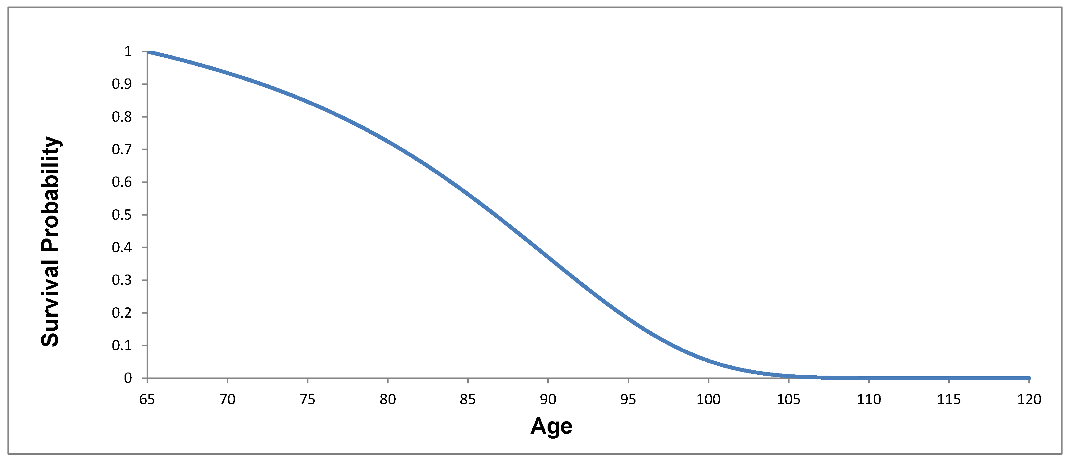
We use this annuity value as our value-based longevity index and construct it on a cohort basis. We make two assumptions to simplify the process of constructing the index. Firstly, we assume that the oldest age is 120. Secondly, starting from initiation, the unit income stream is paid to annuitants who are alive at the end of each year. Based on the model we developed for mortality, we forecast the survival probabilities up to the age of 120. We do not risk adjust our probabilities since we construct the index value based on a best-estimate mortality assumption without risk loadings. At initiation, the survival probability is 100%, and the projected survival curve is monotonically decreasing with age. We also simulate the term structure of interest rates with our interest rate model. Given the estimated number of survivors and discount factors, we calculate the PV as:
where
,
is the estimated expected number of survivors in the annuitant group at the end of year
i and
is the estimated discount factor.
is hence the initial value of the index.
The index value should be updated, and for hedging purposes, we assume this is done on a quarterly basis. Because mortality rates are only available annually, we use linear interpolation for initial mortality rates for fractional ages. The index provides the benchmark value for an immediate annuity for 65-year-olds. It can also be adapted to provide a benchmark value for a deferred annuity for younger ages.
Based on the index, for a group of 65-year-old annuitants today, the annuity provider would require
today if it could fully hedge the longevity risk and interest rate risk. To determine the index, we use the mortality model parameters for the age 65 cohort, age 60 cohort and age 55 cohort. These three cohorts are chosen because the index values we will use will be based on initial ages from 55–65 at five-year intervals. We also project interest rates with the calibrated parameters of the interest rate model. With the estimated survival probabilities and interest rates, we are able to calculate the PV for each index point.
Figure 9 shows the survival probabilities from the mortality model.
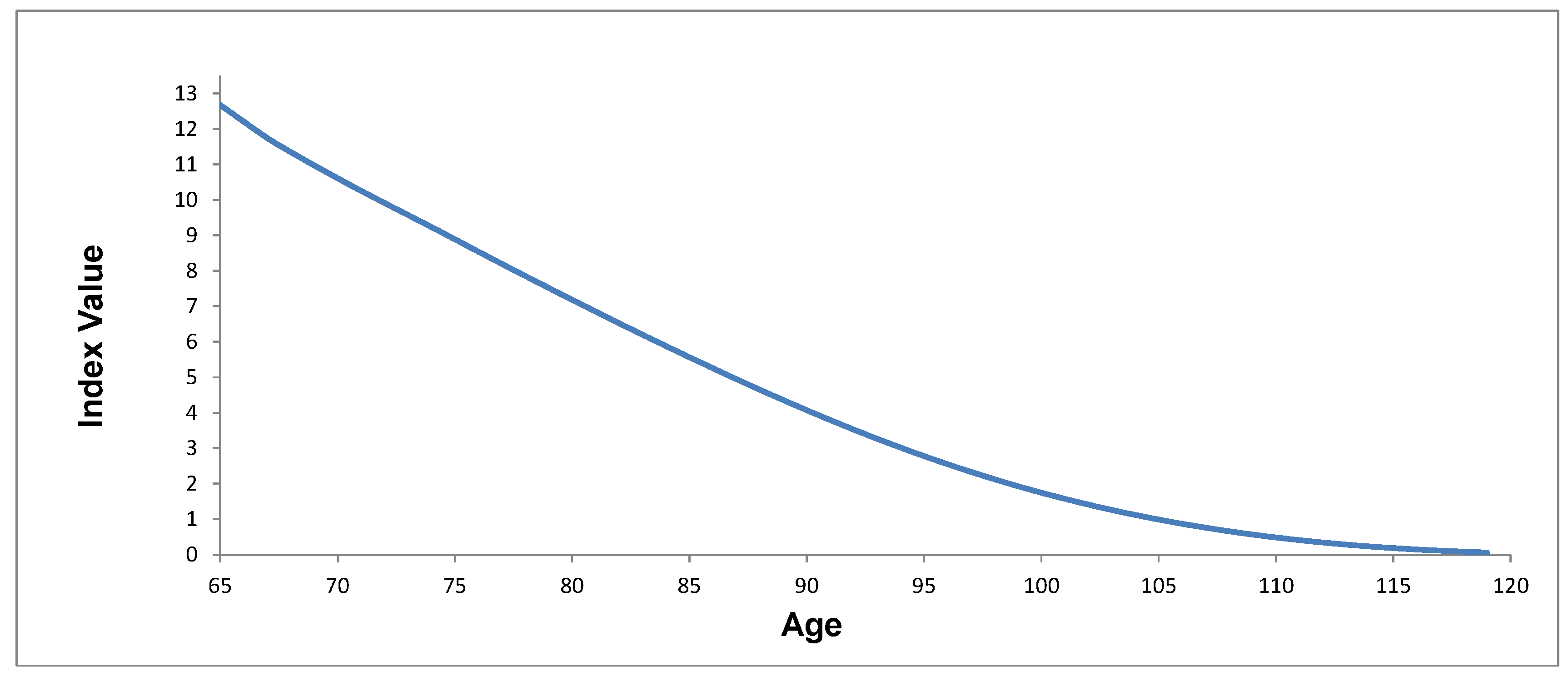
Figure 10 shows the value index.
In
Figure 10 is equal to 12.66. This means that for each individual of the annuity portfolio, the annuity provider needs to invest 12.66 today per unit of income. The index takes a humped shape because it initially increases, then decreases. This is expected because the initial interest rate (observed rate) of each index point firstly decreases, then increases; therefore, the estimated discount factors follow the opposite direction. Although interest rates will be well hedged with the interest rate swaps, the realized survival probabilities will differ from the estimates, so the index is not risk-free even with the interest rate risk hedged and will reflect mortality variations.
The value-based index could be modified to only reflect mortality variations. In theory, this would be achieved by hedging the interest rate risk using a series of interest rate swaps (IRS) with the notional amount adjusted each year to account for mortality. At the beginning of each year of the hedging horizon, an IRS is initiated with a pre-determined notional amount and fixed rate. In the IRS, the annuity provider receives the fixed rate and pays the floating rate. Fixed rates are determined from the projected interest rates. Because the notional amount is invested at floating rates, if the realized number of survivors is exactly the same as estimated, the hedger will have exactly zero cash flow position at the end of the hedging horizon. For the first IRS entered at Time 0, the notional amount is simply
. For the remaining hedging horizon, straightforward calculation shows that the notional amount at the beginning of year
i is:
where
.
is the actual number of deaths, and
is the fixed rate in the swap. This would produce an index that only fluctuated with mortality for the given cohort.
6.2. Hedge Efficiency
With the establishment of the value-based longevity index, we proceed to evaluate its efficiency in hedging value risk for a life annuity provider. We vary the size of a portfolio of annuitants who are Australian males aged 65 at present and evaluate the hedging effectiveness with the index level as the benchmark.
We consider two hedging instruments and compare their efficiencies. The first instrument is a swap in which the annuity provider pays the index value and receives the realized value. With such a swap, the annuity provider is able to transfer the systematic longevity risk and interest rate risk. However, the idiosyncratic longevity risk due to the differences between the portfolio and the population will remain.
The second hedging instrument is a survivor-forward (
LLMA 2010). In the survivor-forward, or s-forward, the annuity provider pays the estimated population survival rate of cohort 65 and receives the realized population survival rate. Hence, the s-forward is only able to hedge the systematic longevity risk, but not the interest rate risk and the idiosyncratic longevity risk. Therefore, the hedge efficiency of the swap with the value index as the underlying relationshould compare favourably to the s-forward.
Our hedging methodology is standard. In order to generate idiosyncratic longevity risk for the portfolio, we follow
Blackburn et al. (
2017) and determine the random death time for each individual in the portfolio for the first time the mortality hazard rate exceeds
, an exponential random variable with parameter one. For each simulation path
m, we keep track of the number of accumulated deaths
at the end of each year
i (
). If the initial number of annuitants of the portfolio is
, then the portfolio survival index at the end of each year
i is:
When evaluating hedge efficiency, the existing literature tends to assume interest rates are constant or deterministic. As a result, the hedge efficiency is likely to be overestimated because interest rate risk is ignored (e.g.,
Coughlan et al. 2011;
Blackburn and Sherris 2014). Suppose we want to hedge the value risk for a portfolio of male annuitants aged 65. We define the hedge efficiency as:
where
and
are respectively the standard deviation of the unexpected PV of the hedged position and the unhedged position.
If we simulate the mortality rates and interest rates with Monte Carlo, then for each path
m, the unexpected value (
) for the unhedged position is:
where
is the simulated PV of path
m for the annuity portfolio allowing for both random future mortality and interest rates. It quantifies the unhedged annuity portfolio variations. These rates capture both aggregate and idiosyncratic mortality. The mortality model generates future stochastic mortality rates, and then for each mortality rate, the random number of deaths is generated.
For the hedged position with the index swap, the annuity provider enters a swap for the annuitant portfolio, and we assume the swap is collateralized and not subject to default risk. In the index swap, the hedger pays the fixed index value
and receives the realized value based on the index. Then, for each path
m, the
is:
where
is the simulated PVof path
m, for the age 65 cohort simulated population survival index with the calibrated mortality model parameters, reflecting only systematic longevity risk. The interest rate risk is hedged by the index swap.
For the hedged position with the s-forward, the
of each simulation path
m is:
where
is the simulated PV at projected population survival probabilities with random interest rates. In general,
because in the s-forward, the interest rate risk is not hedged, only hedging the mortality rate.
Table 10 shows the hedge efficiencies for the two proposed hedging instruments. We vary portfolio size to identify the effect of idiosyncratic longevity risk.
We see that for both instruments, hedge efficiency increases as portfolio size increases. However, the hedge efficiency improvement is more for the index swap than for the s-forward. For a group of 10,000 annuitants, the hedge efficiency is more than 95% for the swap, while less than 70% for the s-forward. This shows that the index swap is the more effective hedging instrument than the s-forward, particularly for a reasonably large portfolio. As discussed earlier in this section, these results are expected because only idiosyncratic longevity risk is retained with the value-based longevity index, which can be reduced by increasing the portfolio size. On the other hand, both idiosyncratic longevity risk and interest rate risk remain with the s-forward, and the latter cannot be reduced with larger portfolios.


