Abstract
We apply spectral biclustering to mortality datasets in order to capture three relevant aspects: the period, the age and the cohort effects, as their knowledge is a key factor in understanding actuarial liabilities of private life insurance companies, pension funds as well as national pension systems. While standard techniques generally fail to capture the cohort effect, on the contrary, biclustering methods seem particularly suitable for this aim. We run an exploratory analysis on the mortality data of Italy, with ages representing genes, and years as conditions: by comparison between conventional hierarchical clustering and spectral biclustering, we observe that the latter offers more meaningful results.
1. Introduction
During the last decade, the analysis of mortality datasets has been deepened by actuaries and statisticians. The growing attention devoted to mortality investigation is due to the financial impact on actuarial liabilities of private life insurance companies, pension funds and national pension systems: as a matter of fact, monthly pension payments are generally based on remaining life expectancy at retirement; the accurate modeling and projection of mortality rates and life expectancy are therefore of growing interest to researchers. In this respect, it makes sense to monitor how much longevity improvements are sizeable: it has been noted that, in the past century survival, probabilities have increased for each age group, even though with some undeniable differences.
As mortality forecasts have become increasingly important, various parametric models have been proposed to describe mortality patterns and produce predictions: in the actuarial literature and practice, the well-known Lee-Carter (LC) model [1] extrapolates the trends of mortality and describes the secular change in longevity as a function of three determinants: the overall time trend, the age component, and the extent of change over time by age. Let us introduce the matrix M = {log mx,t} of log-mortality data for the age x at time t in more detail: x is an integer number in the range [0, 120], and t an integer representing the year of observation (to make an example: m58,2001 is the log-mortality rate recorded in 2001 for individuals 58 years old), so that M has 121 rows and a number of columns depending on the overall number of years for which log-mortality data are available. The model seeks to summarize an age-period surface of log–mortality rates in terms of the vectors a and b along the age dimension, and k along the time dimension: log mx,t = ax + bxkt + εx,t, for every x ∈ [0, 120], and for every t, with restrictions such that the “b”s are normalized to sum to one, the “k”s sum to zero, and the “a”s are average log rates. The vector a can be interpreted as an average age profile, tracking mortality changes over time; the vector b determines how much each age group changes when kt changes. Finally, the error term εx,t reflects age-period effects eventually not captured by the model. In the basic model, the fit to historical data is made through the Singular Value Decomposition (SVD) [2] of M, and then the time-varying parameter is modeled and forecasted as an ARIMA process using standard Box-Jenkins methodology.
As per [3], the diffusion of the LC model is mainly due to its capability to generate realistic life expectancy forecasts; moreover, many developments of the LC method have been suggested (see [4,5]). Furthermore, in the last decade, several authors have proposed approaches to mortality fitting based on smoothing procedures [6,7]; finally, [8] shows a version of the Lee–Carter methodology, the so-called Functional Demographic Model, based on the combination of smoothing techniques and functional data analysis.
More recently, authors have focused attention on mortality patterns of particular generations: increased focus on the size of pension-scheme deficits, in fact, led actuaries to know more about the possible trends in future life span [9]: to such aim, some studies compare the relative influence of both the year of birth and the year of observation, and [10] introduced a variation on the LC model in order to capture the so-called cohort effect, which occurs when a particular generation exhibits patterns of mortality improvements different to those of previous generations. The LC can model the age-period effects; nevertheless, it does not consider the cohort effects, as the analysis of UK data confirms [11]. As a matter of fact, the LC age-period model does not always fit empirical data well (see, for example, [12]), while incorporating the cohort effect into the model sensitively improves the results of the fitting, as well as the comprehension of the mortality evolution. Finally, in the most recent years, a different approach is being experimented to consider the instances and issues highlighted in previous rows; it is based on clustering techniques that are employed to improve the estimation of mortality rates and the cohort effect [13]; in addition, a few number of contributions applied fuzzy logic techniques in mortality projection [14,15]. In particular, [15] applied fuzzy logic to mortality datasets of different countries, capturing the main time effect of the Lee-Carter model for each country.
With respect to the cited literature, our work fits into different research streams, as it extends the application of biclustering techniques, already widely employed to classify gene expression matrices, to the problem of exploring mortality patterns, and it has contact points with the actuarial research strand focused on pattern recognition towards the path already opened by [13]. While, in general, the aim of clustering in genomics is to find gene similarities across all given conditions, in the mortality context, we may assume that the genes are represented by ages and the conditions by years. In the physical world, as with mortality datasets, however, a group of genes often shows similar behavior across just some of the conditions and different properties when looking at others; in these cases, the simple clustering approach is unsuitable for describing the specific patterns in the data. To overcome this limitation, biclustering approaches have been introduced to capture specific patterns in the data even if genes behave similarly over just a subset of conditions ([16,17,18], see also: [19] for a survey). Considering this, as well as the peculiar structure of mortality datasets, we follow the recent actuarial literature on pattern recognition and enhance the clustering approach with the novel introduction of biclustering to analyze mortality data.
In practice, while clusters correspond to disjoint strips in the data matrix, biclusters correspond to arbitrary subsets of rows and columns. To this extent, the notion of bicluster gives rise to a more flexible computational framework. A bicluster can be defined as a submatrix spanned by a set of genes and a set of samples or equivalently, in our case, as the corresponding age and year subsets. Given a mortality matrix, we can therefore characterize the features it embodies by a collection of biclusters, each representing a different type of joint behaviour of a set of ages in a corresponding set of years, without any a priori constraints on the organization of biclusters. The biclustering problem consists then in finding a set of significant biclusters in the data matrix.
Keeping in mind what was stated in previous rows, using biclustering on mortality data should make it possible to identify structural changes in the mortality trend, avoiding the estimation of terms specifically designed to incorporate cohort effects, but rather letting the features of data emerge from the analysis in quite a natural and intuitive way, as we will explain in the section of the paper devoted to describe the methodology. This, in turn, might help to develop more tailored models of mortality forecasting, providing a possibility to compare cohort effects among different countries or groups.
2. Methodological Aspects of Spectral Biclustering
2.1. Biclustering
The goal of clustering is to partition the elements into sets (clusters), while trying to both optimize groups homogeneity (i.e., elements of a cluster should be highly similar to each other), and group separation, which is to say: elements from different clusters should have low similarity to each other. Clustering may be a very powerful tool to automatically detect relevant sub–groups when one does not have prior knowledge about the hidden structure of these data. However, an important issue related to clustering techniques was firstly investigated in the past decade while identifying local patterns in gene expression data: it was highlighted that cluster analysis makes several a priori assumptions [16] that may not be perfectly adequate in all circumstances. As a matter of fact, clustering can be applied to either genes or samples, implicitly directing the analysis to a peculiar aspect of the system under study; in addition, clustering algorithms usually seek a disjoint cover of the set of elements, requiring that no gene or sample belongs to more than one cluster.
The notion of bicluster then gave rise to a more flexible computational framework. Given a gene expression matrix, we can characterize the biological phenomena that it embodies by a collection of biclusters, each representing a different type of joint behavior of a set of genes in a corresponding set of samples. Moreover, as clustering can be separately applied to either the rows or the columns of the data matrix; biclustering, on the other hand, performs clustering in these two dimensions simultaneously. This, in turn, means that while clustering derives a global model, biclustering produces a local model [19]: likewise, in genomics, this aspect is of importance within the mortality context because of the interest of actuaries for age-specific mortality patterns.
As already mentioned in Section 1, in fact, scholars are intended to capture three relevant aspects: the period, the age and the cohort effects, as their knowledge is a key factor in understanding actuarial liabilities of private life insurance companies, pension funds and national pension systems.
2.2. Spectral Biclustering
Following the work of [16], biclustering has quickly become popular in analyzing gene expression data and various biclustering algorithms have been proposed [17,18,19,20,21,22,23,24,25,26]. Since each algorithm focuses on identification of different bicluster patterns, it is a very challenging task to thoroughly evaluate these algorithms.
The rationale inside the spectral biclustering method [27] is that checkerboard structures may emerge in matrices of expression data once they have been properly arranged using a linear algebra approach, by means of the Singular Value Decomposition (SVD). Using SVD, the data matrix D of dimensions N × M can be decomposed as D = UΛVT, where Λ is a diagonal matrix with decreasing non-negative entries, and U and V are orthonormal column matrices with dimensions N × min(N,M) and M × min(N,M), respectively. If the data matrix has a block diagonal structure (with all elements outside the blocks equal to zero), then each block can be associated with a bicluster. Specifically, if the data matrix is of the form:
where Di (i = 1, . . . , k) are arbitrary matrices, then, for each Di, there will be a singular vector pair (ui, vi) such that a nonzero component of ui corresponds to rows occupied by Di, and a nonzero component of vi corresponds to columns occupied by Di.
In a less idealized case, when the elements outside the diagonal blocks are not necessarily zeros but the diagonal blocks still contain dominating values, the SVD can reveal the biclusters as dominating components in the singular vector pairs.
Box 1 illustrates the algorithmic details of the procedure, as reported in [27].
Box 1. Spectral biclustering: the algorithm.
U: conditions; V: genes
DN×M: gene expression matrix.
Compute R = diag(D·1M) and C = diag(1MT D)
Compute SVD of R−1/2 D C−1/2
Discard the pair of eigenvectors corresponding to the largest eigenvalue
For each pair of eigenvectors u,v of R−1DC−1DT and C−1DTR−1D with the same eigenvalue do:
Apply K-means to check the fit of u and v to stepwise vectors
Report the block structure for the p couples u, v with the best stepwise fit.
In our case, the choice of the biclustering method was suggested by the analogies existing between spectral biclustering and the Singular Value Decomposition on which the Lee–Carter method [1]—LCm—is based.
Furthermore, the starting point of the introduction of biclustering method in mortality context is to design a clustering approach suitable for the kind of data we are working on. Most biclustering algorithms, in fact, are apt to binary data only, and, therefore, they are not appropriate for mortality rates. Instead, spectral biclustering appears suitable for death rates matrix because it finds the checkerboard structure in data through the extraction of significant eigenvectors using the SVD associated to some normalization steps; this approach is also in line with the most used approach for fitting mortality data, the LCm, based on the SVD of the mortality matrix. Moreover, the normalization step reduces the effects of random differences in experimental conditions and levels of genes, and it is useful to highlight biclusters, if a structure exists. Finally, as a common practice in biclustering analysis is transforming the data by taking logarithms, we believe the log-normalization is appropriate in a mortality context because two or more ages are experiencing the same evolution if their mortality profiles are constantly proportional, and the log-transformation is not affected by an additive constant.
3. Discussion Case
The structural description of mortality table constitutes the base to understand mortality patterns and to derive an opportune mortality model to fit and project historical data; our research aims to identify every demographic feature in mortality data, capturing both the so-called period and age effects: the former is related to the evolution of life expectancy during the years, the latter to the differences of mortality across ages. Recently, demographers and actuaries have focused their attention on a third effect, the so-called cohort effect, looking for generations that show particular mortality patterns. Without an ex-ante investigation of the structure of data, the demographical models are often worsened with cohort parameters to capture generational effect, while the interaction of age–time effects in the data structure could be misunderstood and, for example, wrongly attributed to the cohort effect. For this reason, a preliminary investigation of data becomes useful to design a parsimonious mortality model.
While the microarray technology is a central tool in biological studies, it is an unexplored field in demographic context, where the identification of individuals with similar mortality patterns represents a key step in the analysis of life tables. However, traditional clustering algorithms, like the hierarchical one, organize the mortality matrix into submatrices assuming that all genes behave similarly in groups of conditions, but it would be unreasonable in the mortality context.
The biclustering methods are useful to find meaningful checkerboard patterns in matrices where data represent marker genes expressed under a particular set of conditions; they permit simultaneously clustering genes and conditions. In the mortality datasets, the genes are represented by ages and the conditions by years: we observe how the mortality for individuals aged differently has changed under different conditions, i.e., as time changes.
The aim of biclustering is therefore to highlight groups of mortality rates in which ages are clustered together if they exhibit similar patterns across years and, likewise, years are clustered together if they include ages whose mortality has shown a similar evolution. In this way, it is possible to discover homogeneous submatrices that are relevant for understanding mortality evolution in social and actuarial studies.
3.1. Demographical Settings and Notational Conventions
In the context of mortality data, demographers and actuaries work on life tables. A life table is a finite decreasing sequence l0, l1, ... , lω where lx refers to an integer age x and represents the estimated number of people alive at x in a given population composed by l 0 individuals aged 0 at inception; note that ω commonly indicates the so-called extreme age, representing the age at which it occurs: lω = 0: for sake of convenience, we can assume ω = 120. A cohort table is obtained if the sequence l0, l1, ... , lω is the longitudinal observation of the actual numbers of individuals alive at ages 1, 2, . . . , ω out of a given initial cohort of l0 newborns. If we consider an existing population and observe the frequency of death at different ages in a given period, for example, one year, then we obtain the period table. Finally, M = {log mij} is usually employed to denote the matrix of death rates of a particular population, where the data are organized in rows by age, and in columns by years, so that mi,j is the mortality rate at the age i (i = 0, . . . ,ω) in the year j.
3.2. Empirical Results
In our case study, we considered the death rates of the whole (male and female) Italian population; the data were downloaded from the Human Mortality Database 1 (HMD). The genes are represented by ages collected between 40 and 60, and the conditions by the years between 1950 and 2006. We focus on the ages in the range [40, 60] because those ages are the most important in pensions and actuarial product design.
We applied to data both the hierarchical Euclidean clustering (whose algorithm is provided in Appendix A, at the end of the paper) and the spectral biclustering, already explained in Box 1 of Section 2, and visualized the results through heatmaps.
The first step of our analysis consists in grouping the data through a Euclidean hierarchical cluster method; we applied the algorithm to the columns and rows of death rates matrix separately, and Figure 1 and Figure 2 show the corresponding heat maps.
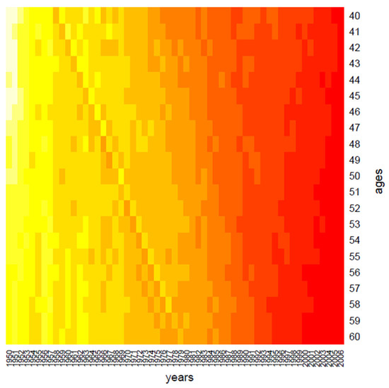
Figure 1.
Clustering: the period effect.
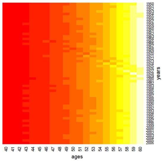
Figure 2.
Clustering: the age effect.
Clustering performs data in one dimension at a time, so each gene in a given gene cluster is defined using all the conditions, and, similarly, each condition in a condition cluster is characterized by the activity of all the genes that belong to it. From a graphical point of view, this produces vertical regions that appear in Figure 1 and Figure 2, where the period effect and the age effect become visible: moving from yellow regions to red regions, the mortality decreases during years and increases across ages. We also highlight the presence of the cohort effect, as some generations have experienced specific mortality patterns differently from others. If the cohort effect is present, a kind of “ladder” appears in the heatmap: genes aged x in t, x + 1 in t + 1, and so on are grouped in the same cluster and are represented with the same color shade in the heatmap.
In more detail, in Figure 1, we may observe a diagonal line, corresponding to the individuals aged 40 in 1958, i.e., the generation born in 1918; such graphical evidence suggests that this group has experienced a particular reduction in mortality during the years.
However, it is not reasonable that groups of genes behave similarly under all conditions; it could occur, for example, that group of ages show similar features just during some years, and they cluster differently during other years. To capture this detailed structure, we introduce the biclustering as a useful tool to find meaningful checkerboard patterns.
In the second step of our application, we have therefore randomly applied the spectral biclustering algorithm to the matrix of mortality rates, normalized through the log-transformation, thus obtaining 20 clusters: main results are visually summarized in Figure 3, Figure 4, Figure 5, Figure 6 and Figure 7. Above all, the heat map of Figure 3 shows not only vertical regions, but also rectangular areas produced by the interaction between age and period effects.
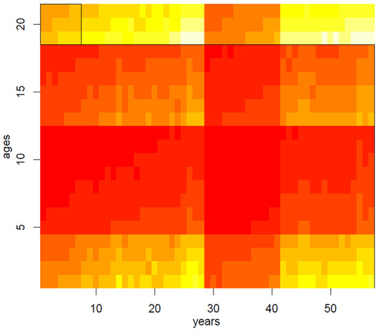
Figure 3.
Biclustering on the mortality dataset.
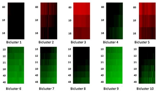
Figure 4.
Biclusters 1–10.
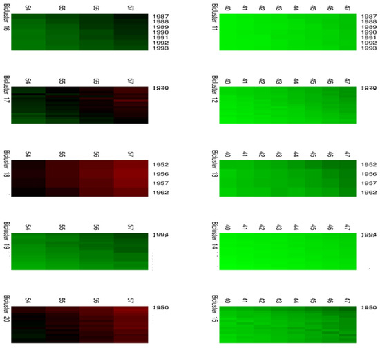
Figure 5.
Biclusters 11–20.
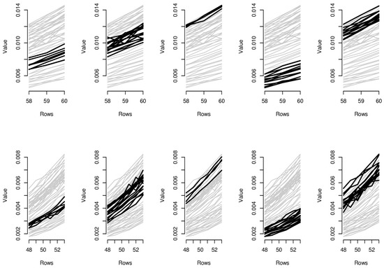
Figure 6.
Parallel coordinate graphs for biclusters 1–10.
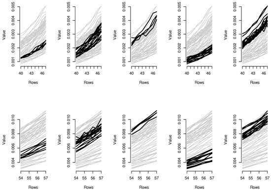
Figure 7.
Parallel coordinate graphs for biclusters 11–20.
Moreover, Figure 4 and Figure 5 highlight the composition of each bicluster, summarized in Table 1: four groups of ages (40–47, 48–53, 54–57, 58–60) are defined, each of them characterized by significant patterns across particular years. For example, the first bicluster contains ages 58–60 during the years 1987–1993; the same ages act differently during the years 1970–1986 and are grouped in the second bicluster, and so on.

Table 1.
The composition of biclusters.
In order to provide the reader with additional interpretative keys, in Figure 6 and Figure 7, we show parallel coordinate graphs for mortality levels.
Let us take a look, for instance, at the first two clusters including the levels of mortality between the ages 58 and 60 during the years 1987–1993 and 1987–1993. In the parallel coordinate graphs, the light gray lines represent the mortality for each year of the whole dataset, while the bold lines represent the level of mortality for each year included in the bicluster. By a mutual comparison of the lines in the first two boxes of Figure 7, we can note that the mortality between the ages 58–60 moving from the period 1970–1986 to the period 1987–1993 has sensitively decreased. In particular, we can note the effect of the reduction of mortality trend during the period 1950–2006, looking in sequence at box 5-2-1-4 of Figure 7. The years included in the third bicluster represent an exception to the general trend, probably due to accidental deviations in the mortality trend. In the actuarial practice, it is well known that the demographic risk can be split into two components: the insurance risk and the longevity risk. The former arises from accidental deviations of the number of deaths from its expected trend, while the latter derives from systematic improvements in the mortality trend. It is possible to improve mortality forecasts removing the accidental deviations from the dataset on which the fitting and forecasts are implemented and the bicluster method can be useful to this scope.
Similar considerations can be easily extended to the other biclusters; for instance, as it is clear from biclusters 4-9-14-19, in Figure 6 and Figure 7, all ages have experimented a reduction from the mortality trend during the last two decays.
We also checked the statistical significance and the stability of the applied biclustering technique. To this aim, F-statistics are calculated from the two-way ANOVA mode with the row and column effect; low p-values denote non-random selection of columns for a given bicluster. We have calculated the F-statistics for each cluster and have obtained p-values of almost zero for both row and column effects. Table 2 shows the p-values of the F-statistics corresponding to the row and column effects.
Table 2.
The p-values of the F-statistics from the two-way ANOVA.
Moreover, for each cluster, Constant and Additive Variances are calculated, as one can see in Table 3. They represent measures of how a bicluster is coherent, following [19], and return the corresponding variance of genes or conditions as the average of the sum of Euclidean distances between all rows and columns of the bicluster. The lower the values returned, the more constant or coherent the bicluster is. If the value returned is near 0, the bicluster is ideally constant or coherent. Usually, a value above 1–1.5 is enough to determine if the bicluster is not constant or coherent.
Table 3.
Constant and additive variance.
4. Conclusions
In this paper, we discussed the use of biclustering techniques to discover patterns in mortality data tables. This approach can be motivated by the attention devoted to mortality investigations: the accurate modeling and projection of mortality rates and life expectancy, in fact, are of growing interest to researchers because of their impact on actuarial liabilities of private life insurance companies, pension funds and national pension systems; in this respect, it makes sense to monitor the extent to which the longevity improvements is meaningful.
Our work therefore nests in at least two research strands. The first research vein deals with biclustering: to the best of our knowledge, this is a first-time application, with spectral biclustering applied to a classification problem where the role of genes is played by individuals’ ages, and the time to represent condition. Furthermore, we show that using spectral biclustering instead of standard clustering techniques presents several advantages, as in this way it is possible to capture demographical effects that are generally disregarded by other techniques. An example in such sense is offered by the so-called cohort effect that occurs when it is possible to identify generations exhibiting particular mortality patterns and where condition is represented by time: without proper ex ante investigations of the mortality data structure, the demographical models are often worsened with cohort parameters to capture generational effect, while the interaction of age–time effect in the data structure could be misunderstood and, for example, wrongly attributed to the cohort effect. In this respect, a preliminary investigation of data with biclustering methods becomes useful to design a parsimonious mortality model.
However, as biclustering algorithms are mostly apt to binary data, they are not always appropriate to deal with mortality rates. Nevertheless, the spectral biclustering appears suitable for a death rates matrix because it finds the checkerboard structure in data through the extraction of significant eigenvectors using the SVD associated with some normalization steps; this approach is also in line with the most used approach for fitting mortality data.
In our case study, we applied spectral biclustering to the death rates of the whole (male and female) Italian population, with genes represented by ages collected between 40 and 60, and the conditions by the years between 1950 and 2006. We applied both the hierarchical clustering and the spectral biclustering, and visualized the results through heat maps. By visual comparison of the results, we highlighted that the spectral biclustering was able both to capture effects lost in the case of standard clustering, and to correctly address the significance of existing patterns, as testified by the analysis of biclusters’ coherence.
However, we are aware that the scope of the clusterization and biclusterization technique is not to explain why certain patterns occur, but to identify patterns in the data. They are unsupervised learning methods: the results of clustering algorithms are data driven, and, for this reason, they explain better the underlying structure of the data. This represents an advantage, but also a drawback: without a possibility to tell the system what to do like in other supervised methods, it is often difficult to explain clustering results. Every method has advantages and drawbacks, and the choice of a particular one depends on the scope of the research. The biclusterization we have proposed could be useful for a preliminary investigation of the mortality dataset, before implementing a stochastic model for the mortality projections. In fact, the widely used stochastic mortality models, like the Lee–Carter model, are based on time series extrapolation, and the results are influenced by the historical series considered and the estimation window. Projections change considerably according to the age and years considered, and the biclusters could represent important preliminary information about how data have to be included in the projections.
We can therefore conclude that biclustering can offer a useful technique to run exploratory analysis of mortality datasets, as a prelude to the construction of an efficient and parsimonious model of mortality. Steps for future works include the possibility to fit some well-known mortality models separately on different biclusters and verify the potential improvements in the fitting with an opportune analysis of the residuals. The biclustering approach can also offer useful preliminary information for the segmentation of the pension and insurance market.
Acknowledgments
The authors would like to thank the reviewers for insightful comments and suggestions, which led to a much improved manuscript.
Author Contributions
Gabriella Piscopo and Marina Resta conceived and designed the paper; Marina Resta illustrated the algorithms; Gabriella Piscopo developed the application.
Conflicts of Interest
The authors declare no conflict of interest.
Appendix A: The Euclidean Hierarchical Clustering Method
We assume to have a set of N items to be clustered, and an N × N distance matrix whose components are calculated by evaluating the Euclidean distance between each couple of item. Then, the basic process of hierarchical clustering (as defined by [28]) works as follows:
- Assigning each item to a cluster, so that if you have N items, you now have N clusters, each containing just one item. The distances between the clusters are assumed to be the same as the distances (similarities) between the items they contain.
- Find the closest (i.e., the most similar) pair of clusters and merge them into a single cluster, hence reducing by one the original number of clusters, as defined in 1.
- Compute the distances between the new cluster and each of the old clusters.
- Repeat steps 2 and 3 until the items are clustered into the desired number k of clusters.
References
- D. Lee, and L. Carter. “Modeling and Forecasting U.S. Mortality.” J. Am. Stat. Assoc. 87 (1992): 659–671. [Google Scholar] [CrossRef]
- G. Golub, and C. Van Loan. Matrix Computations, 3rd ed. Baltimore MD, USA: Johns Hopkins University Press, 1996. [Google Scholar]
- H. Booth, R. Hyndman, and L. Tickle. “Lee-Carter mortality forecasting: A multi-country comparison of variants and extensions.” Demogr. Res. 15 (2006): 289–310. [Google Scholar] [CrossRef]
- H. Booth, J. Maindonald, and L. Smith. “Applying Lee-Carter under conditions of variable mortality decline.” Popul. Stud. 56 (2002): 325–336. [Google Scholar] [CrossRef] [PubMed]
- Z. Butt, S. Haberman, R. Verrall, and V. Wass. “Calculating compensation for loss of earnings: Estimating and using work life expectancy.” J. R. Stat. Soc. Ser. A 171 (2008): 763–805. [Google Scholar] [CrossRef]
- A. Delwarde, M. Denuit, and P. Eilers. “Smoothing the Lee-Carter and Poisson log-bilinear models for mortality forecasting. A penalized loglikelihood approach.” Stat. Model. 7 (2007): 29–48. [Google Scholar] [CrossRef]
- I. Currie, M. Durban, and P. Eilers. “Smoothing and forecasting mortality rates.” Stat. Model. 4 (2004): 279–298. [Google Scholar] [CrossRef]
- R. Hyndman, and S. Ullah. “Robust forecasting of mortality and fertility rates: A functional data approach.” Comput. Stat. Data Anal. 51 (2007): 4942–4956. [Google Scholar] [CrossRef]
- S. Richards. “Understanding Pensioner Longevity.” The Actuary Magazine, 26–27 May 2007. [Google Scholar]
- A. Renshaw, and S. Haberman. “A cohort-based extension to the Lee-Carter model for mortality reduction factors.” Insur. Math. Econ. 38 (2006): 556–570. [Google Scholar] [CrossRef]
- R. Willets. “The cohort effect: Insights and explanations.” Br. Actuar. J. 10 (2004): 833–877. [Google Scholar] [CrossRef]
- A. Renshaw, and S. Haberman. Lee-Carter Mortality Forecasting Incorporating Bivariate Time Series. Actuarial Research Paper 153; London, UK: Faculty of Actuarial Science Insurance, City University London, 2003. [Google Scholar]
- Y. Leong, and J. Yu. “A Spatial Cluster Modification of the Lee-Carter Model.” In Proceedings of the Longevity Risks 8, Cass Business School, London, UK, 7–8 September 2012. [Google Scholar]
- C. Skiadas, and C. Skiadas. “A Modeling Approach to Life Table Data Sets.” In Recent Advances in Stochastic Modeling and Data Analysis. Singapore, Singapore: World Scientific, 2007, pp. 350–359. [Google Scholar]
- P. Hatzopoulos, and S. Haberman. “Common mortality modelling and coherent forecasts. An empirical analysis of worldwide mortality data.” Insur. Math. Econ. 52 (2013): 320–337. [Google Scholar] [CrossRef]
- Y. Cheng, and G. Church. “Biclustering of expression data.” In Proceedings of the International Conference on Intelligent Systems for Molecular Biology, San Diego, CA, USA, 19–23 August 2000; Volume 8, pp. 93–103. [Google Scholar]
- J. Ihmels, G. Friedlander, S. Bergmann, O. Sarig, and Y. Ziv. “Revealing Modular Organization in the Yeast Transcriptional Network.” Nat. Genet. 31 (2002): 370–377. [Google Scholar] [CrossRef] [PubMed]
- T. Murali, and S. Kasif. “Extracting conserved gene expression motifs from gene expression data.” In Proceedings of the Pacific Symposium on Biocomputing, Kauai, HI, USA, 3–7 January 2003; Volume 8, pp. 77–88. [Google Scholar]
- S. Madeira, and A. Oliveira. “Biclustering algorithms for biological data analysis: A survey.” IEEE/ACM Trans. Comput. Biol. Bioinform. 1 (2004): 24–45. [Google Scholar] [CrossRef] [PubMed]
- E. Segal, B. Taskar, A. Gasch, N. Friedman, and D. Koller. “Rich probabilistic models for gene expression.” Bioinformatics 17 (2001): S243–S252. [Google Scholar] [CrossRef] [PubMed]
- A. Tanay, R. Sharan, and R. Shamir. “Discovering statistically significant biclusters in gene expression data.” Bioinformatics 18 (2002): 136–144. [Google Scholar] [CrossRef]
- H. Wang, W. Wang, J. Yang, and P. Yu. “Clustering by Pattern Similarity in Large Data Sets.” In Proceedings of the 2002 ACM SIGMOD International Conference on Management of Data, Madison, WI, USA, 3–6 June 2002; pp. 394–405. [Google Scholar]
- D. Jiang, J. Pei, and A. Zhang. “DHC: A density-based hierarchical clustering method for time series gene expression data.” In Proceedings of the IEEE International Symposium on Bioinformatics and Bioengineering, Bethesda, MD, USA, 12 March 2003; pp. 393–400. [Google Scholar]
- J. Liu, and W. Wang. “Op-cluster: Clustering by tendency in high dimensional space.” In Proceedings of the IEEE International Conference on Data Mining, Melbourne, FL, USA, 22 November 2003; p. 187. [Google Scholar]
- J. Gu, and J. Liu. “Bayesian biclustering of gene expression data.” BMC Genom. 9 (2008): S4. [Google Scholar] [CrossRef] [PubMed]
- G. Li, Q. Ma, H. Tang, A. Paterson, and Y. Xu. “QUBIC: A qualitative biclustering algorithm for analyses of gene expression data.” Nucleic Acids Res. 37 (2009): e1015. [Google Scholar] [CrossRef] [PubMed]
- Y. Kluger, R. Basri, J. Chang, and M. Gerstein. “Spectral biclustering of microarray data: Coclustering genes and conditions.” Genome Res. 13 (2003): 703–716. [Google Scholar] [CrossRef] [PubMed]
- S.C. Johnson. “Hierarchical clustering schemes.” Psychometrika 3 (1967): 241–254. [Google Scholar] [CrossRef]
© 2017 by the authors. Licensee MDPI, Basel, Switzerland. This article is an open access article distributed under the terms and conditions of the Creative Commons Attribution (CC BY) license ( http://creativecommons.org/licenses/by/4.0/).