Compositions of Conditional Risk Measures and Solvency Capital

Abstract

In this paper, we consider compositions of conditional risk measures in order to obtain time-consistent dynamic risk measures and determine the solvency capital of a life insurer selling pension liabilities or a pension fund with a single cash-flow at maturity. We first recall the notion of conditional, dynamic and time-consistent risk measures. We link the latter with its iterated property, which gives us a way to construct time-consistent dynamic risk measures from a backward iteration scheme with the composition of conditional risk measures. We then consider particular cases with the conditional version of the value at risk, tail value at risk and conditional expectation measures. We finally give an application of these measures with the determination of the solvency capital of a pension liability, which offers a fixed guaranteed rate without any intermediate cash-flow. We assume that the company is fully hedged against the mortality and underwriting risks.

1. Introduction

The determination of the economic capital of a life insurer or pension fund has become of paramount importance over the past decade due to the recent financial crisis in the banking sector. The management and measurement of risk is of great interest, as can be seen from the recent Basel II and III regulatory frameworks for banks and Solvency II for the European insurance sector. These new regulations are designed to be risk sensitive. The Solvency II regulation recognizes that the insurer faces different kinds of risks, like market and longevity risks, while the previous regulation (Solvency I) is factor based. These regulations use risk measures as introduced in [1,2,3] in order to quantify the riskiness of financial positions and to provide a criterion to determine their acceptability. For instance, the new Solvency II framework requires a value at risk (VaR) measure to determine the solvency capital requirement, while the Swiss Solvency Test uses the tail value at risk (TVaR) measure for its target capital. These measures consider a real-valued random variable describing a future financial value and measure its risk at the beginning of the time period. Under the Solvency II and the Swiss Solvency Test regulations, the length of the time period is equal to one year, i.e., these frameworks consider the evolution of their own funds of the insurance undertaking over one year. However, life insurers and pension funds hold also long-term products, such as pension liabilities, which are the topic of this paper.

In this paper, we consider pension liabilities, and we study risk measures that consider the long-term characteristic of these products. We focus here on the market risk, especially the equity risk. We also assume that the company is fully hedged against the mortality and underwriting risks.

An important drawback of the classic static risk measures is that they do not take into account the information disclosed through time. These measures only consider the end-points of the time period. If we deal with liabilities with a maturity of one year, then these risk measures are adapted as we work with a time horizon equal to the accounting horizon. Because we consider pension liabilities with a long-term horizon, this information could be meaningful in the computation of the solvency capital through time, especially on a yearly basis, as is the case for accounting purposes. That is why we consider dynamic risk measures as studied in [3,4,5,6]. The information is modeled by a filtration, and this filtration is incorporated in the computation of the capital each year.

A first example of a dynamic risk measure could be the recalculated version of the static risk measures. We could for instance recalculate the solvency capital each year according to a static risk measure by incorporating the information available. However, this approach only incorporates past information, and for well-known measures, such as the VaR or TVaR measures, this could lead to time inconsistency, i.e., a position that was acceptable could become undesirable in any scenario. Therefore, we require a particularly useful property for dynamic risk measures, which is called time consistency. This property tells us that if we prefer a position tomorrow in almost every state of the world, then we already prefer it today. It is well known that the recalculated versions of the VaR and TVaR measures are not time consistent (see [7,8]).

It has been proven that a time-consistent dynamic risk measure is closely linked to a backward iteration scheme [9]. We then consider this property to construct time-consistent risk measures through the iteration of conditional risk measures. This approach has been considered for the determination of the solvency capital of life insurance products in [10,11,12]. Nevertheless, it appears that the solvency capital obtained can be very expensive if we do not take care of the confidence level of each conditional VaR and TVaR measures involved in the iteration scheme. This is linked to a result obtained in [13], which tells us that, under certain hypotheses, if we consider a great number of iterations, the risk measure obtained is close to either the conditional expectation of the risk or its essential supremum.

In order to overcome this difficulty, we consider the iterations of different conditional risk measures with a yearly time step fitting the accounting point of view. We also build these measures in such a way that they are coherent with the Solvency II or Swiss Solvency Test frameworks, meaning that for the last year of the product, the measures we introduce here correspond to the one used in these frameworks.

This paper then introduces a new way to compute the solvency capital in life insurance, in order to take into account simultaneously the following three constraints

• to be in line with Solvency II on a one-year horizon;
• to be time consistent;
• to incorporate in the risk measurement the maturity of the product.

The paper is organized as follows. We set the mathematical framework in Section 2. Then, we recall the definition of conditional and dynamic risk measures in Section 3, of time consistency and iterated risk measures in Section 4 and present some compositions of conditional risk measures in order to determine the solvency capital in Section 5. We then compute the solvency capital in Section 6 and finally give a numerical illustration in Section 7.

2. Framework

Throughout the paper, we consider a complete atomless probability space $(\mathsf{\Omega },\mathcal{F},\mathbb{P})$. We write ${\mathbb{N}}^{*}=\mathbb{N}\backslash \left\{0\right\}$. We fix $T\in {\mathbb{N}}^{*}$ seen as the maturity of a pension liability and define $\mathbb{T}=\{0,\dots ,T-1\}$ as the set of intermediate dates. We also consider a filtration:

$$\mathbb{F}={\left({\mathcal{F}}_t\right)}_{t\in \mathbb{T}\cup \left\{T\right\}},$$

such that ${\mathcal{F}}_0=\{\varnothing ,\mathsf{\Omega }\}$ and ${\mathcal{F}}_T=\mathcal{F}$. All inequalities and equalities between random variables (r.v.’s) are meant to hold $\mathbb{P}$-almost surely ($\mathbb{P}$-a.s.) if not stated otherwise. Let $t\in \mathbb{T}\cup \left\{T\right\}$. We define ${\mathrm{L}}^1(\mathsf{\Omega },{\mathcal{F}}_t,\mathbb{P})$ as the space of all real-valued ${\mathcal{F}}_t$-measurable r.v.’s X, such that $\mathbb{E}\left[\right|X\left|\right]<+\infty$, where two r.v.’s are identified if they coincide a.s. We consider an equivalence class $X\in {\mathrm{L}}^1(\mathsf{\Omega },{\mathcal{F}}_t,\mathbb{P})$ as a r.v., and we understand X as a financial amount at date t of date t money. We also identify ${\mathrm{L}}^1(\mathsf{\Omega },{\mathcal{F}}_0,\mathbb{P})$ with $\mathbb{R}$.

3. Conditional and Dynamic Risk Measures

We consider dynamic risk measures in order to determine the solvency capital of a pension liability. The solvency capital is the amount the company has to put aside, in addition to the initial value of its portfolio, in order to be solvent. The idea behind dynamic risk measures is to consider the amount of information available through time. In our setting, this amount of information is modeled by the filtration $\mathbb{F}$.

Let $t\in \mathbb{T}$. We consider a reference instrument ${\iota }_{t,T}\in {\mathrm{L}}^1(\mathsf{\Omega },{\mathcal{F}}_T,\mathbb{P})$, as introduced in [1] in the static case. The amount ${\iota }_{t,T}$ is the value at time T of one unit of currency invested in this reference instrument between time t and T. The solvency capital computed at date t is then invested in this financial instrument ${\iota }_{t,T}$ from date t to the maturity T. We assume that ${\iota }_{t,T}\left(\omega \right)>0$ for all $\omega \in \mathsf{\Omega }$. This reference instrument could be a risk-free zero-coupon bond, and the value at time T would be:

$${\iota }_{t,T}=\frac{1}{P(t,T)},$$

where $P(t,T)$ is the price of a risk-free zero-coupon bond at time t with maturity T and paying one unit of currency.

We first recall the definition of a conditional risk measure. In the following, we understand $X\in {\mathrm{L}}^1(\mathsf{\Omega },{\mathcal{F}}_T,\mathbb{P})$ as a profit r.v., which means that if $X\left(\omega \right)<0$, then the company faces a loss at maturity T under scenario $\omega \in \mathsf{\Omega }$; otherwise, it makes a profit.

Definition 1.

A conditional risk measure ${\rho }_t$ on ${\mathrm{L}}^1(\mathsf{\Omega },{\mathcal{F}}_T,\mathbb{P})$ with a reference instrument ${\iota }_{t,T}$ is a function:

$${\rho }_t:{\mathrm{L}}^1(\mathsf{\Omega },{\mathcal{F}}_T,\mathbb{P})⟶{\mathrm{L}}^1(\mathsf{\Omega },{\mathcal{F}}_t,\mathbb{P}),$$

such that it satisfies the following properties, for $X,Y\in {\mathrm{L}}^1(\mathsf{\Omega },{\mathcal{F}}_T,\mathbb{P})$,

• (monotonicity) $X\le Y$ implies ${\rho }_t\left(X\right)\ge {\rho }_t\left(Y\right)$;
• (conditional cash invariance) for all $m_t\in {\mathrm{L}}^1(\mathsf{\Omega },{\mathcal{F}}_t,\mathbb{P})$,

  $${\rho }_t(X+m_t{\iota }_{t,T})={\rho }_t\left(X\right)-m_t;$$
• (normalization) ${\rho }_t\left(0\right)=0$.

We can also define convex and coherent conditional risk measures as in the classic static setting.

Definition 2.

A conditional risk measure ${\rho }_t$ on ${\mathrm{L}}^1(\mathsf{\Omega },{\mathcal{F}}_T,\mathbb{P})$ is called convex if for $X,Y\in {\mathrm{L}}^1(\mathsf{\Omega },{\mathcal{F}}_T,\mathbb{P})$ and $\lambda \in {\mathrm{L}}^1(\mathsf{\Omega },{\mathcal{F}}_t,\mathbb{P})$, $0\le \lambda \le 1$,

$${\rho }_t\left(\lambda X+(1-\lambda )Y\right)\le \lambda {\rho }_t\left(X\right)+(1-\lambda ){\rho }_t\left(Y\right).$$

Furthermore, ${\rho }_t$ is called coherent if it is convex and, for $X\in {\mathrm{L}}^1(\mathsf{\Omega },{\mathcal{F}}_T,\mathbb{P})$ and $\lambda \in {\mathrm{L}}^1(\mathsf{\Omega },{\mathcal{F}}_t,\mathbb{P})$, $\lambda \ge 0$,

$${\rho }_t\left(\lambda X\right)=\lambda {\rho }_t\left(X\right).$$

A dynamic risk measure is simply a sequence of conditional risk measures.

Definition 3.

A dynamic risk measure:

$$\rho ={\left({\rho }_t\right)}_{t\in \mathbb{T}}$$

on ${\mathrm{L}}^1(\mathsf{\Omega },{\mathcal{F}}_T,\mathbb{P})$ is a sequence of conditional risk measures ${\rho }_t$ on ${\mathrm{L}}^1(\mathsf{\Omega },{\mathcal{F}}_T,\mathbb{P})$ (with the reference instrument ${\iota }_{t,T}$), for $t\in \mathbb{T}$. It is called convex (resp.coherent) if ${\rho }_t$ is convex (resp. coherent) for all $t\in \mathbb{T}$.

Remark 1.

We refer the reader to [3,4,5,6] for a detailed study of this kind of measure.

For $X\in {\mathrm{L}}^1(\mathsf{\Omega },{\mathcal{F}}_T,\mathbb{P})$ seen as a final net worth at date T of a life insurer or pension fund and $t\in \mathbb{T}$, the amount ${\rho }_t\left(X\right)$ (which is an r.v.) can be seen as a solvency capital at date t of date t money for the final net worth X, which is invested in the reference instrument ${\iota }_{t,T}$ over the period $[t,T]$, i.e.,

$${\rho }_t\left(X+{\rho }_t\left(X\right){\iota }_{t,T}\right)=0,$$

by the conditional cash invariance property, where we recall that this equality holds in the $\mathbb{P}$-a.s. sense.

4. Time Consistency and Iterated Risk Measures

A time-consistent risk measure tells us that if we prefer a position tomorrow, in almost all states of nature, then we already prefer it today (see [4,5], for instance).

Definition 4.

A dynamic risk measure ρ on ${\mathrm{L}}^1(\mathsf{\Omega },{\mathcal{F}}_T,\mathbb{P})$ is called time consistent if:

$${\rho }_{t+1}\left(X\right)\le {\rho }_{t+1}\left(Y\right),$$

implies:

$${\rho }_t\left(X\right)\le {\rho }_t\left(Y\right),$$

for all $t\in \mathbb{T}$, $t\ne T-1$ and $X,Y\in {\mathrm{L}}^1(\mathsf{\Omega },{\mathcal{F}}_T,\mathbb{P})$.

Example 1.

In order to understand why this property is important, in particular in the field of a pension liability, we consider two r.v.’s X and Y described in Figure 1. While in Section 2, we consider an atomless probability space, we set here for the purpose of the example a discrete probability space $(\mathsf{\Omega },\mathcal{F},\mathbb{P})$.

The set of states of nature Ω is given by:

$$\mathsf{\Omega }=\{{\omega }_1,{\omega }_2,{\omega }_3,{\omega }_4\},$$

with the σ-algebra $\mathcal{F}$ given by:

$$\mathcal{F}=\mathcal{P}\left(\mathsf{\Omega }\right),$$

and a probability measure $\mathbb{P}$ given by:

$$\begin{array}{cc}\hfill \mathbb{P}\left[\left\{{\omega }_1\right\}\right]& =0.01\times 0.01=0.0001\hfill \\ \hfill \mathbb{P}\left[\left\{{\omega }_2\right\}\right]& =0.01\times 0.99=0.0099\hfill \\ \hfill \mathbb{P}\left[\left\{{\omega }_3\right\}\right]& =0.99\times 0.01=0.0099\hfill \\ \hfill \mathbb{P}\left[\left\{{\omega }_4\right\}\right]& =0.99\times 0.99=0.9801.\hfill \end{array}$$

We consider two periods, i.e., we set $T=2$. We then define a filtration $\mathbb{F}={\left({\mathcal{F}}_t\right)}_{t\in \{0,1,2\}}$ with:

$$\begin{array}{cc}\hfill {\mathcal{F}}_0& =\{\varnothing ,\mathsf{\Omega }\}\hfill \\ \hfill {\mathcal{F}}_1& =\sigma \left(\{{\omega }_1,{\omega }_2\},\{{\omega }_3,{\omega }_4\}\right)\hfill \\ \hfill {\mathcal{F}}_2& =\mathcal{F}.\hfill \end{array}$$

This filtration means that at time $t=1$, we know if we are at node $\{{\omega }_1,{\omega }_2\}$ or $\{{\omega }_3,{\omega }_4\}$, i.e., at time $t=1$, we know that two scenarios are possible, either ${\omega }_1$ and ${\omega }_2$ or ${\omega }_3$ and ${\omega }_4$. We also compute that:

$$\begin{array}{cc}\hfill \mathbb{P}\left[\left\{{\omega }_1\right\}\right|\{{\omega }_1,{\omega }_2\}]& =0.01\hfill \\ \hfill \mathbb{P}\left[\left\{{\omega }_2\right\}\right|\{{\omega }_1,{\omega }_2\}]& =0.99\hfill \\ \hfill \mathbb{P}\left[\left\{{\omega }_3\right\}\right|\{{\omega }_3,{\omega }_4\}]& =0.01\hfill \\ \hfill \mathbb{P}\left[\left\{{\omega }_4\right\}\right|\{{\omega }_3,{\omega }_4\}]& =0.99.\hfill \end{array}$$

We see X and Y as two possible outcomes (strategies) for our life insurer or pension fund at time $T=2$. For instance, if we follow the strategy of X, we see that at time $t=1$, if we are at node $\{{\omega }_1,{\omega }_2\}$, the probability of facing a loss of 250 is $1\%$. We emphasize that when X or Y are positive, the company faces a profit, while it faces a loss when X or Y are negative. That is why the amount of the loss is 250, while X takes as a value $-250$. We assume here that ${\iota }_{0,2}={\iota }_{1,2}=1$, so that we neglect the time value of money for this example.

We consider the VaR measure with a level of 99% in order to make a choice between X and Y. We first compute the VaR measure with a confidence level of 99% at time $t=0$ (see [1,3]),

$$\begin{array}{cc}\hfill {\mathrm{VaR}}_0^{0.99}\left(X\right)& =-inf\left\{x\in \mathbb{R}:\mathbb{P}\left[X\le x\right]>0.01\right\}\hfill \\ & =10,\hfill \end{array}$$

and:

$$\begin{array}{c}\hfill {\mathrm{VaR}}_0^{0.99}\left(Y\right)=5,\end{array}$$

which means that at time $t=0$, we prefer Y over X, because:

$$\begin{array}{c}\hfill {\mathrm{VaR}}_0^{0.99}\left(X\right)>{\mathrm{VaR}}_0^{0.99}\left(Y\right).\end{array}$$

However, at time $t=1$, we compute that, if we are at node $\{{\omega }_1,{\omega }_2\}$,

$$\begin{array}{cc}\hfill \left.{\mathrm{VaR}}_1^{0.99}\left(X\right)\right|\{{\omega }_1,{\omega }_2\}& =-inf\left\{x\in \mathbb{R}:\mathbb{P}\left[X\le x\left|\right\{{\omega }_1,{\omega }_2\}\right]>0.01\right\}\hfill \\ & =10,\hfill \end{array}$$

and:

$$\begin{array}{c}\hfill \left.{\mathrm{VaR}}_1^{0.99}\left(Y\right)\right|\{{\omega }_1,{\omega }_2\}=50;\end{array}$$

and, at node $\{{\omega }_3,{\omega }_4\}$,

$$\begin{array}{cc}\hfill \left.{\mathrm{VaR}}_1^{0.99}\left(X\right)\right|\{{\omega }_3,{\omega }_4\}& =-inf\left\{x\in \mathbb{R}:\mathbb{P}\left[X\le x\left|\right\{{\omega }_3,{\omega }_4\}\right]>0.01\right\}\hfill \\ & =-5,\hfill \end{array}$$

and:

$$\begin{array}{cc}\hfill \left.{\mathrm{VaR}}_1^{0.99}\left(Y\right)\right|\{{\omega }_3,{\omega }_4\}& =5,\hfill \end{array}$$

which means that at time $t=1$, we now prefer X over Y, because:

$${\mathrm{VaR}}_1^{0.99}\left(X\right)<Va{R}_1^{0.99}\left(Y\right),$$

while we chose Y at time $t=0$ (see Figure 2 for a summary). It is clear that at time $t=1$, the strategy Y appears riskier than strategy X. If the dynamic (recalculated) version of the VaR measure was time consistent, we would not have faced such an inconsistent behavior over time. That is why we believe that a time-consistent measure is needed.

For instance, let us consider the conditional expectation. We compute that:

$$\mathbb{E}[-X]=-3.29<5.2=\mathbb{E}[-Y],$$

so that we prefer X over Y at time $t=0$. Then, at time $t=1$, we compute that:

$$\mathbb{E}\left.\left[-X\right|\{{\omega }_1,{\omega }_2\}\right]=12.4<54.5=\mathbb{E}\left.\left[-Y\right|\{{\omega }_1,{\omega }_2\}\right],$$

and:

$$\mathbb{E}\left.\left[-X\right|\{{\omega }_3,{\omega }_4\}\right]=-3.45<4.7=\mathbb{E}\left.\left[-Y\right|\{{\omega }_3,{\omega }_4\}\right],$$

which means that at time $t=1$, we still prefer X over Y (see Figure 3 for a summary). According to this measure, the choice of X is constant over time, because this measure is time consistent.

Remark 2.

We also refer to [11] for another example and [8] for an example with an atomless probability space.

Time-consistent risk measures are closely-linked to iterated risk measures.

Definition 5.

A dynamic risk measure ρ on ${\mathrm{L}}^1(\mathsf{\Omega },{\mathcal{F}}_T,\mathbb{P})$ is called iterated if:

$${\rho }_t\left(X\right)={\rho }_t\left(-{\rho }_{t+1}\left(X\right){\iota }_{t+1,T}\right),$$

for $t\in \mathbb{T}$, $t\ne T-1$ and $X\in {\mathrm{L}}^1(\mathsf{\Omega },{\mathcal{F}}_T,\mathbb{P})$.

Theorem A1 of Appendix A tells us that time-consistent and iterated risk measures are equivalent and then that a time-consistent risk measure can be computed following a backward iteration scheme. Furthermore, it also gives us a way to construct time-consistent risk measures following this backward iteration scheme. This is formalized in Corollary 1. Section 5 aims at designing suitable time-consistent risk measures by means of this result.

Corollary 1.

Let γ be a dynamic risk measure on ${\mathrm{L}}^1(\mathsf{\Omega },{\mathcal{F}}_T,\mathbb{P})$ that is not time consistent. Then, the dynamic risk measure ρ on ${\mathrm{L}}^1(\mathsf{\Omega },{\mathcal{F}}_T,\mathbb{P})$ given by:

$${\rho }_{T-1}\left(X\right)={\gamma }_{T-1}\left(X\right),$$

and:

$${\rho }_t\left(X\right)={\gamma }_t\left(-{\rho }_{t+1}\left(X\right){\iota }_{t+1,T}\right),$$

for all $t\in \mathbb{T}$, $t\ne T-1$, is time consistent. Furthermore, if γ is convex (resp. coherent), then ρ is also convex (resp. coherent).

5. Compositions of Conditional Risk Measures

While classic static risk measures have been considered to determine the solvency capital of a financial institution (see, for instance, [1,3]), we would now like to consider dynamic risk measures and, more precisely, time-consistent dynamic risk measures in order to determine the solvency capital of a life insurer or pension fund. A first study of this approach can be found in [10,11,12], where they consider iterated versions of the conditional VaR or TVaR measures. However, it appears clear that the levels of the solvency capital are quite expensive (about equal to the present value of the liability for long maturities in some cases).

This observation is related to ([13] [Theorem 1.10]). Following this result, they assume a certain class of dynamic risk measures, i.e., law-invariant, and a great number of iterations, i.e., they consider $\mathbb{T}=\mathbb{N}$, which means that a countably infinite number of steps is considered. Then, under these hypotheses, the dynamic risk measure obtained is given by a sequence of conditional entropic risk measures. In particular, if the dynamic measure is assumed coherent, then the solvency capital would be given by either the expected value of the final net worth or its largest possible value, its essential supremum.

The difference between the approach of ([13] [Theorem 1.10]) and the one we present here lies in the number of iterations. We consider here T iterations, i.e., a finite number of steps $t\in \mathbb{T}$ (see Corollary 1), while in ([13] [Theorem 1.10]) they consider an infinite (but still countable) number of iterations, i.e., $t\in \mathbb{N}$. However, depending on the choice of the dynamic risk measure and on the actual final net worth considered, a great number of iterations T could converge towards ([13] [Theorem 1.10]), which is the case in [10,11,12].

The idea behind this section is to consider a yearly basis for the computation of the solvency capital and to be careful of the confidence level considered within each iteration. If we reduce the time step (for instance, with a weekly or daily basis, without considering its practicability), then we will tend toward the previous observation because, due to the long-term characteristic of our pension products (typically 45 years), we would obtain a great number of iterations (about 2340 with a weekly-step over 45 years). This yearly time step is based on an accounting point of view and allows us to develop some time-consistent risk measures that could fit the Solvency II or Swiss Solvency Test frameworks in the last year of the product.

In Section 5.1, we consider the composition of conditional VaR measures, while in Section 5.2, we consider the case with conditional TVaR measures. Finally, in Section 5.3, we construct a time-consistent measure from the composition of either a conditional VaR measure or a conditional TVaR measure and conditional expectations.

5.1. Composition of VaRs

We begin this section with the definition of a conditional VaR measure (see [3]).

Definition 6.

Let $t\in \mathbb{T}$ and $\alpha \in (0,1)$. The conditional VaR measure on ${\mathrm{L}}^1(\mathsf{\Omega },{\mathcal{F}}_T,\mathbb{P})$ with the confidence level α is defined by:

$$\begin{array}{c}\hfill {\mathrm{VaR}}_t^{\alpha }\left(X\right)=-ess\; inf\left\{V\in {\mathrm{L}}^1(\mathsf{\Omega },{\mathcal{F}}_t,\mathbb{P}):\mathbb{P}\left[X\le V{\iota }_{t,T}|{\mathcal{F}}_t\right]>1-\alpha \mathrm{a}.\mathrm{s}.\right\},\end{array}$$

for $X\in {\mathrm{L}}^1(\mathsf{\Omega },{\mathcal{F}}_T,\mathbb{P})$, where ess inf stands for the essential infimum as defined in [3].

We are now able to define the dynamic generalization of the classic static VaR measure, the recalculated VaR measure, which is simply the sequence of conditional VaR measures.

Definition 7.

The recalculated VaR measure on ${\mathrm{L}}^1(\mathsf{\Omega },{\mathcal{F}}_T,\mathbb{P})$ with a confidence level $\alpha \in (0,1)$ is defined by the sequence:

$${\mathrm{VaR}}^{\alpha }={\left({\mathrm{VaR}}_t^{\alpha }\right)}_{t\in \mathbb{T}}.$$

This dynamic risk measure does not fulfill the useful property of time consistency and is even not convex.

Proposition 1.

Let $\alpha \in (0,1)$. The dynamic risk measure ${\mathrm{VaR}}^{\alpha }$ on ${\mathrm{L}}^1(\mathsf{\Omega },{\mathcal{F}}_T,\mathbb{P})$ is neither convex nor time consistent.

Proof. 

For the convexity, take for instance $t=0$, and for the time consistency, see ([3] [Example 11.13]). ☐

Let $\mathit{\alpha }\in {(0,1)}^T$, i.e.,

$$\mathit{\alpha }=\left({\alpha }_1,\dots ,{\alpha }_T\right),$$

with ${\alpha }_i\in (0,1)$ for $i\in \{1,\dots ,T\}$. We define an iterated measure according to this vector, by means of conditional VaR measures. This vector is a vector of confidence levels, which could be different. The iterated measure is then a composition of different conditional (VaR) measures.

Definition 8.

Let $\mathit{\alpha }\in {(0,1)}^T$. For $X\in {\mathrm{L}}^1(\mathsf{\Omega },{\mathcal{F}}_T,\mathbb{P})$, the iterated VaR (IVaR) measure on ${\mathrm{L}}^1(\mathsf{\Omega },{\mathcal{F}}_T,\mathbb{P})$ is given by,

$$\begin{array}{c}\hfill {\mathrm{IVaR}}_{T-1}^{\mathit{\alpha }}\left(X\right)={\mathrm{VaR}}_{T-1}^{{\alpha }_1}\left(X\right),\end{array}$$

and:

$$\begin{array}{c}\hfill {\mathrm{IVaR}}_t^{\mathit{\alpha }}\left(X\right)={\mathrm{VaR}}_t^{{\alpha }_{T-t}}\left(-{\mathrm{IVaR}}_{t+1}^{\mathit{\alpha }}\left(X\right){\iota }_{t+1,T}\right),\end{array}$$

for $t\in \mathbb{T}$, $t\ne T-1$.

Remark 3.

It is clear that this measure is a dynamic risk measure that is time consistent, because the sequence:

$${\left({\mathrm{VaR}}_t^{{\alpha }_{T-t}}\right)}_{t\in \mathbb{T}}$$

defines a dynamic risk measure, and Corollary 1 allows us to conclude.

Remark 4.

For a given $\alpha \in (0,1)$ and ${\alpha }_i=\alpha$, for all $i\in \{1,\dots ,T\}$, this case has been considered in [8,12]. However, it appears in [12] that this dynamic measure gives expensive solvency capital. This is due to ([13] [Theorem 1.10]) and the observation made at the beginning of this section. Instead of considering the same α within each iteration, we propose here to make it dependent on the date $t\in \mathbb{T}$ of valuation.

Remark 5.

If we set ${\alpha }_1=99.5\%$, then this time-consistent dynamic risk measure is consistent with the Solvency II framework. For a product with a time to maturity of one year or, more generally, for the last year of a product, we get back the SIIframework, since we then only consider a VaR at a level of 99.5% over one year.

5.2. Composition of TVaRs

We can also consider the case of the iterated TVaR measure, which will give us a coherent and time-consistent risk measure. We recall the definition of the conditional TVaR measure (see ([3] [Proposition 11.9])).

Definition 9.

Let $t\in \mathbb{T}$ and $\alpha \in (0,1)$. For $X\in {\mathrm{L}}^1(\mathsf{\Omega },{\mathcal{F}}_T,\mathbb{P})$, the conditional TVaR measure on ${\mathrm{L}}^1(\mathsf{\Omega },{\mathcal{F}}_T,\mathbb{P})$ with the confidence level α is defined by,

$$\begin{array}{c}\hfill {\mathrm{TVaR}}_t^{\alpha }\left(X\right)={\mathrm{VaR}}_t^{\alpha }\left(X\right)+\frac{1}{1-\alpha }\mathbb{E}\left[\left.{\left(\frac{X}{{\iota }_{t,T}}+{\mathrm{VaR}}_t^{\alpha }\left(X\right)\right)}_{-}\right|{\mathcal{F}}_t\right],\end{array}$$

where ${(·)}_{-}=-min(·,0)$.

Its corresponding dynamic risk measure is not time consistent.

Definition 10.

The recalculated TVaR measure on ${\mathrm{L}}^1(\mathsf{\Omega },{\mathcal{F}}_T,\mathbb{P})$ with a confidence level $\alpha \in (0,1)$ is defined by the sequence:

$${\mathrm{TVaR}}^{\alpha }={\left({\mathrm{TVaR}}_t^{\alpha }\right)}_{t\in \mathbb{T}}.$$

Proposition 2.

Let $\alpha \in (0,1)$. The dynamic risk measure ${\mathrm{TVaR}}^{\alpha }$ on ${\mathrm{L}}^1(\mathsf{\Omega },{\mathcal{F}}_T,\mathbb{P})$ is coherent, but not time consistent.

Proof. 

It is clearly coherent from the classic properties of the conditional expectation. Concerning the time consistency, we refer to ([3] [Example 11.13]). ☐

Again, we consider Corollary 1 in order to construct a time-consistent version.

Definition 11.

Let $\mathit{\alpha }\in {(0,1)}^T$. The iterated TVaR (ITVaR) measure on ${\mathrm{L}}^1(\mathsf{\Omega },{\mathcal{F}}_T,\mathbb{P})$ is given by, for $X\in {\mathrm{L}}^1(\mathsf{\Omega },{\mathcal{F}}_T,\mathbb{P})$,

$$\begin{array}{c}\hfill {\mathrm{ITVaR}}_{T-1}^{\mathit{\alpha }}\left(X\right)={\mathrm{TVaR}}_{T-1}^{{\alpha }_1}\left(X\right),\end{array}$$

and:

$$\begin{array}{c}\hfill {\mathrm{ITVaR}}_t^{\mathit{\alpha }}\left(X\right)={\mathrm{TVaR}}_t^{{\alpha }_{T-t}}\left(-{\mathrm{ITVaR}}_{t+1}^{\mathit{\alpha }}\left(X\right){\iota }_{t+1,T}\right),\end{array}$$

for $t\in \mathbb{T}$, $t\ne T-1$.

Remark 6.

Following Remark 5, if we set ${\alpha }_1=99\%$, then this time-consistent dynamic risk measure is also consistent with the Swiss Solvency Test.

5.3. Composition with Conditional Expectations

In this section, we define a time-consistent dynamic measure as the composition of either a conditional VaR measure or a conditional TVaR measure and conditional expectations. We start by giving the definition of a conditional expectation measure.

Definition 12.

Let $t\in \mathbb{T}$. The conditional expectation measure ${\mathrm{E}}_t$ on ${\mathrm{L}}^1(\mathsf{\Omega },{\mathcal{F}}_T,\mathbb{P})$ is defined by,

$$\begin{array}{c}\hfill {\mathrm{E}}_t\left(X\right)=\mathbb{E}\left[\left.-\frac{X}{{\iota }_{t,T}}\right|{\mathcal{F}}_t\right],\end{array}$$

for $X\in {\mathrm{L}}^1(\mathsf{\Omega },{\mathcal{F}}_T,\mathbb{P})$.

We now give the definition of the composition of a conditional VaR measure and conditional expectation measures. We construct it by means of Corollary 1, and we call it the expected VaR measure. With the first iteration, we consider a usual conditional VaR measure, then through the following steps, we consider its expected value.

Definition 13.

Let $\alpha \in (0,1)$. The expected VaR (EVaR) measure ${\mathrm{EVaR}}^{\alpha }$ on ${\mathrm{L}}^1(\mathsf{\Omega },{\mathcal{F}}_T,\mathbb{P})$ with the confidence level α is given by:

$$\begin{array}{c}\hfill {\mathrm{EVaR}}_{T-1}^{\alpha }\left(X\right)={\mathrm{VaR}}_{T-1}^{\alpha }\left(X\right),\end{array}$$

and:

$$\begin{array}{c}\hfill {\mathrm{EVaR}}_t^{\alpha }\left(X\right)={\mathrm{E}}_t\left(-{\mathrm{EVaR}}_{t+1}^{\alpha }\left(X\right){\iota }_{t+1,T}\right),\end{array}$$

for $t\in \mathbb{T}$, $t\ne T-1$ and $X\in {\mathrm{L}}^1(\mathsf{\Omega },{\mathcal{F}}_T,\mathbb{P})$.

Remark 7.

Again, following Remark 5, if we set $\alpha =99.5\%$, this time consistent dynamic risk measure is consistent with the Solvency II framework. The first iteration is the same as with the IVaR measure. However, the difference between the IVaR and EVaR measures is in the following steps, where we consider now the conditional expected measure.

We also consider the expected TVaR measure.

Definition 14.

Let $\alpha \in (0,1)$. The expected TVaR (ETVaR) measure $\mathrm{E}{\mathrm{TVaR}}^{\alpha }$ on ${\mathrm{L}}^1(\mathsf{\Omega },{\mathcal{F}}_T,\mathbb{P})$ with the confidence level α is given by:

$$\begin{array}{c}\hfill {\mathrm{ETVaR}}_{T-1}^{\alpha }\left(X\right)={\mathrm{TVaR}}_{T-1}^{\alpha }\left(X\right),\end{array}$$

and:

$$\begin{array}{c}\hfill {\mathrm{ETVaR}}_t^{\alpha }\left(X\right)={\mathrm{E}}_t\left(-{\mathrm{ETVaR}}_{t+1}^{\alpha }\left(X\right){\iota }_{t+1,T}\right),\end{array}$$

for $t\in \mathbb{T}$, $t\ne T-1$ and $X\in {\mathrm{L}}^1(\mathsf{\Omega },{\mathcal{F}}_T,\mathbb{P})$.

We see that this definition is a particular case of Definition 11. If we consider the vector $\mathit{\alpha }\in {(0,1)}^T$ in Definition 11 with:

$${\alpha }_i=\left\{\begin{array}{cc}\alpha \hfill & \mathrm{if}i=1\hfill \\ 0\hfill & \mathrm{if}i>1\hfill \end{array}\right.,$$

then we get back Definition 14.

Remark 8.

We emphasize that the order considered in Definitions 13 and 14 is important. In the first step, we consider the conditional VaR or TVaR measure, and then, we use the conditional expectation for the subsequent steps. This means that for the last year of the product, or equivalently, when the time to maturity is equal to one, we get back the classic VaR or TVaR.

However, if we chose the conditional expectation for $t=1,\dots ,T-1$ and used the VaR or TVaR for $t=0$, then we would get a completely different time-consistent measure. For the last year of the product, the capital would be given by the conditional expectation only and not by a VaR or TVaR. This is due to the fact that each year t, when we recompute the solvency capital, we do not consider anymore the measure used at time $t-1$.

6. Solvency Computation

The purpose of this section is to study the impact of the equity risk on the solvency capital computed by means of the measures previously defined. The inclusion of the interest rate and longevity risks has been considered in [14] with static risk measures. However, the inclusion of these risks in our dynamic setting would require the use of numerical techniques in order to compute the solvency capital, while the framework that we consider here allows us to obtain closed-form formulae. For instance, considering a simple Vasicek model for the short-term interest rate would gives us differences between log-normally-distributed random variables.

In Section 6.1, we set the pension liability of the life insurer or pension fund. We define its assets in Section 6.2, its final net worth in Section 6.3 and consider its solvency capital in Section 6.4.

6.1. Liabilities

We consider a life insurer or pension fund that offers a fixed guaranteed rate $r_G\in \mathbb{R}$ over a time horizon $T\in {\mathbb{N}}^{*}$. We assume that the company is fully hedged against the mortality and underwriting risks. Then, the liability at maturity is given by:

$$L_T={\pi }_0{e}^{r_{G}T},$$

where ${\pi }_0\in \mathbb{R}$ is the initial unique contribution paid for the affiliate.

Remark 9.

This corresponds to a defined contribution with a minimum guaranteed rate or a cash-balance plan. However, we could have considered a defined benefit (DB) plan, as well. Results in Propositions 3, 4 and 5 are sufficiently general to allow easy adaptations when liabilities and interest rate are deterministic.

6.2. Assets

We assume a financial market modeled by a Black–Scholes–Merton model [15,16] with $r\in \mathbb{R}$ the constant risk-free interest rate, a bank account and a stock. The contribution ${\pi }_0$ is invested in a portfolio A over the period $[0,T]$ made up of these assets and which follows a constant proportion allocation strategy, i.e., its stochastic differential equation (SDE) is given by, for $t\in [0,T]$,

$$\mathrm{d}{A}_t=\left(\theta \mu +(1-\theta )r\right)A_t\mathrm{d}t+\theta \sigma A_t\mathrm{d}{W}_t,$$

where $\theta \in [0,1]$ is the deterministic proportion of the portfolio invested in the stock, W is a standard Brownian motion, $A_0={\pi }_0$, $\mu ,\sigma \in \mathbb{R}$ and $\sigma >0$. Therefore, at any time $t\in [0,T]$, a proportion θ of the portfolio $A_t$ is invested in the stock, and a proportion $1-\theta$ is invested in the bank account. We then have:

$$\begin{array}{c}\hfill A_t={\pi }_{0}exp\left[\left(\theta \mu +(1-\theta )r-\frac{{\theta }^2{\sigma }^2}{2}\right)t+\theta \sigma W_t\right],\end{array}$$

(1)

for all $t\in [0,T]$.

As the term structure is flat and known with certainty, the price at time $t\in [0,T]$ of a zero-coupon bond paying one unit of currency at maturity $s\in [0,T]$, $t\le s$, is given by:

$$P(t,s)=e^{-r(s-t)}.$$

6.3. Final Net Worth

The final net worth (at maturity T) of the pension liability is simply given by the difference between its final assets and liabilities, i.e., given by the r.v.:

$${\mathrm{FNW}}_T=A_T-{\mathrm{L}}_T.$$

For $\omega \in \mathsf{\Omega }$, the company faces a loss at maturity under scenario ω if:

$${\mathrm{FNW}}_T\left(\omega \right)<0,$$

otherwise, it is solvent.

6.4. Solvency Capital

We define the solvency capital as the amount the company has to put aside, in addition to the initial value of its portfolio, in order to be solvent at maturity according to a particular measure. This amount at time $t\in \mathbb{T}$ is invested in a product ${\iota }_{t,T}$ over the period $[t,T]$. We consider here:

$${\iota }_{t,T}=\frac{1}{P(t,T)},$$

which means that the solvency capital at time t is invested in a zero-coupon bond between dates t and T. This choice for the reference instrument can be considered as prudent. For instance, we could have decided to invest the solvency capital in the portfolio of assets, i.e.,

$${\iota }_{t,T}=\frac{A_T}{A_t},$$

which is clearly riskier. This approach has been considered in [12] where it is observed that the solvency capital computed according to this investment strategy is higher than the prudent approach of a risk-free zero-coupon bond.

The solvency capital given by the iterated VaR and TVaR measures (see Definitions 8 and 11) is computed as follows.

Proposition 3.

Let $\mathit{\alpha }\in {(0,1)}^T$. We compute that:

$$\begin{array}{c}{\mathrm{IVaR}}_t^{\mathit{\alpha }}\left({\mathrm{FNW}}_T\right)\hfill \\ \hfill =L_{T}P(t,T)-P(t,T)A_{t}exp\left[\left(\theta \mu +(1-\theta )r-\frac{{\theta }^2{\sigma }^2}{2}\right)(T-t)+\theta \sigma \sum _{i=1}^{T-t}{\mathsf{\Phi }}^{-1}\left(1-{\alpha }_i\right)\right],\end{array}$$

(2)

and:

$$\begin{array}{c}\hfill {\mathrm{ITVaR}}_t^{\mathit{\alpha }}\left({\mathrm{FNW}}_T\right)=L_{T}P(t,T)-P(t,T)A_{t}exp\left[\left(\theta \mu +(1-\theta )r\right)(T-t)\right]\prod _{i=1}^{T-t}\left[\frac{\mathsf{\Phi }\left({\mathsf{\Phi }}^{-1}\left(1-{\alpha }_i\right)-\theta \sigma \right)}{1-{\alpha }_i}\right],\end{array}$$

for $t\in \mathbb{T}$, where Φ denotes the cumulative distribution function of a standard normal r.v., i.e., for $y\in \mathbb{R}$,

$$\mathsf{\Phi }\left(y\right)=\frac{1}{\sqrt{2\pi }}{\int }_{-\infty }^y{e}^{-\frac{x^2}{2}}\mathrm{d}x,$$

and ${\mathsf{\Phi }}^{-1}$ its inverse.

Proof. 

See Appendix B. ☐

Remark 10.

For both the iterated VaR and TVaR measures, we observe that the solvency capital is a decreasing function of μ, while it is increasing with σ. Furthermore, for the iterated VaR, the first derivative with respect to μ is a decreasing function, meaning that the speed of decrease will increase with μ, while the first derivate with respect to σ is an increasing function.

We also consider the solvency capital given by the expected VaR and TVaR measures (see Definitions 13 and 14).

Proposition 4.

Let $\alpha \in (0,1)$. We compute that:

$$\begin{array}{c}\hfill {\mathrm{EVaR}}_t^{\alpha }\left({\mathrm{FNW}}_T\right)=L_{T}P(t,T)-P(t,T)A_{t}exp\left[\left(\theta \mu +(1-\theta )r\right)(T-t)-\frac{{\theta }^2{\sigma }^2}{2}+\theta \sigma {\mathsf{\Phi }}^{-1}\left(1-\alpha \right)\right],\end{array}$$

and:

$$\begin{array}{c}\hfill {\mathrm{ETVaR}}_t^{\alpha }\left({\mathrm{FNW}}_T\right)=L_{T}P(t,T)-P(t,T)A_{t}exp\left[\left(\theta \mu +(1-\theta )r\right)(T-t)\right]\frac{\mathsf{\Phi }\left({\mathsf{\Phi }}^{-1}\left(1-\alpha \right)-\theta \sigma \right)}{1-\alpha },\end{array}$$

for $t\in \mathbb{T}$.

Proof. 

Similar to the proof of Proposition 3. ☐

If we compare Propositions 3 and 4, we see that the iterated VaR (resp. TVaR) considers a sequence of bad events, while the expected VaR (resp. TVaR) only considers one bad event affecting the last year of the product (the first iteration). The expected VaR (resp. TVaR) incorporates a security margin in the first iteration, for the last year of the product. However, the iterated VaR (resp. TVaR) can incorporate a security margin in each iteration, according to the confidence level considered at each step. For instance, we could consider a linearly-decreasing margin when the number of iterations increases (see examples below). We could then consider the expected VaR or TVaR as a lower bound for the solvency capital.

Finally, we compare this solvency capital with that obtained by means of the recalculated risk measures.

Proposition 5.

Let $\alpha \in (0,1)$. We compute that:

$$\begin{array}{c}\hfill {\mathrm{VaR}}_0^{\alpha }\left({\mathrm{FNW}}_T\right)=L_{T}P(0,T)-P(0,T)A_{0}exp\left[\left(\theta \mu +(1-\theta )r-\frac{{\theta }^2{\sigma }^2}{2}\right)T+\theta \sigma \sqrt{T}{\mathsf{\Phi }}^{-1}\left(1-\alpha \right)\right],\end{array}$$

and:

$$\begin{array}{c}\hfill {\mathrm{TVaR}}_0^{\alpha }\left({\mathrm{FNW}}_T\right)=L_{T}P(0,T)-P(0,T)A_{0}exp\left[\left(\theta \mu +(1-\theta )r\right)T\right]\frac{\mathsf{\Phi }\left({\mathsf{\Phi }}^{-1}\left(1-\alpha \right)-\theta \sigma \sqrt{T}\right)}{1-\alpha }.\end{array}$$

Proof. 

We only consider one step in the proof of Proposition 3. ☐

7. Numerical Illustration

In this section, we consider different values for $\mathit{\alpha }\in {(0,1)}^T$ and $\alpha \in (0,1)$ in order to compute the solvency capital. We only compare the initial values of the solvency capital, i.e., $t=0$.

We assume that $T\in \{1,\dots ,45\}$, $\theta =40\%$, so that $40\%$ of the portfolio is invested in the stock, that the guaranteed interest rate is equal to the risk free rate, i.e., $r_G=r$, and that ${\pi }_0=1000$€. Concerning the financial market, the stock has been calibrated on daily log returns of the Belgian BEL20 index from 2 April 1991 to 31 December 2013 by means of the maximum likelihood estimation (MLE) method (see

Table 1. Parameters of the GBMobtained by the MLE method with the corresponding standard errors between brackets.

μ	σ
$0.05564$ ($0.03827$)	$0.18415$ ($0.00172$)

). We also set the constant interest rate to $1.5\%$.

In order to be consistent with either a Solvency II or a Swiss Solvency Test approach, we will consider:

$${\alpha }^{\left(\mathrm{SII}\right)}=0.995,$$

when working with VaR measures and:

$${\alpha }^{\left(\mathrm{SST}\right)}=0.99,$$

for TVaR measures.

We first define the confidence levels in the case of the recalculated measures of Proposition 5. We follow the maturity approach as introduced in [10] and set:

$${\alpha }^1={\left({\alpha }^{\left(\mathrm{SII}\right)}\right)}^T,$$

and:

$${\alpha }^2={\left({\alpha }^{\left(\mathrm{SST}\right)}\right)}^T.$$

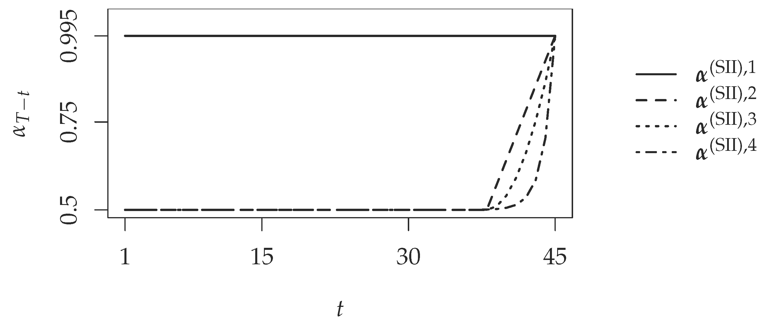
We also consider four definitions for the vector $\mathit{\alpha }\in {(0,1)}^T$ for the VaR and TVaR cases. We write for the j-th definition, $j\in \{1,\dots ,4\}$,

$${\mathit{\alpha }}^{\left(\mathrm{SII}\right),j}={\left({\alpha }_i^{\left(\mathrm{SII}\right),j}\right)}_{i\in \{1,\dots ,T\}},$$

when dealing with VaR measures and:

$${\mathit{\alpha }}^{\left(\mathrm{SST}\right),j}={\left({\alpha }_i^{\left(\mathrm{SST}\right),j}\right)}_{i\in \{1,\dots ,T\}},$$

for TVaR measures. We give an illustration of these definitions in Figure 4 for the SII case.

The first one is the constant case, which is also studied in [12],

$${\alpha }_i^{\left(\mathrm{SII}\right),1}={\alpha }^{\left(\mathrm{SII}\right)},$$

and:

$${\alpha }_i^{\left(\mathrm{SST}\right),1}={\alpha }^{\left(\mathrm{SST}\right)},$$

for $i\in \{1,\dots ,T\}$.

For the three others definitions, we consider an integer $K>0$. We see this parameter as the maturity after which we consider that a product is a long-term product, for instance $K=8$ years.

The second definition follows a linear increase when the time to maturity is decreasing, i.e., when i decreases,

$${\alpha }_i^{\left(\mathrm{SII}\right),2}=\left\{\begin{array}{cc}{\alpha }^{\left(\mathrm{SII}\right)}-\frac{{\alpha }^{\left(\mathrm{SII}\right)}-0.5}{K-1}(i-1)\hfill & \mathrm{if}i<K\hfill \\ 0.5\hfill & \mathrm{if}i\ge K\hfill \end{array}\right.,$$

and:

$${\alpha }_i^{\left(\mathrm{SST}\right),2}=\left\{\begin{array}{cc}{\alpha }^{\left(\mathrm{SST}\right)}-\frac{{\alpha }^{\left(\mathrm{SST}\right)}-1}{K-1}(i-1)\hfill & \mathrm{if}i<K\hfill \\ 0\hfill & \mathrm{if}i\ge K\hfill \end{array}\right.,$$

for $i\in \{1,\dots ,T\}$. We see that the confidence parameter decreases linearly towards either 50% or 0% within K years and afterwards stays constant. We chose 50% for the measures based on the VaR in order to obtain either the mean of the solvency capital if its distribution is symmetric or its median if not. With 0% for the measures based on the TVaR, we obtain directly the mean of the solvency capital. These choices are linked with the EVaR and ETVaR measures where the decrease is instantaneous ($K=1$). In other words, for a time to maturity greater than K years, the parameter stays constant while it starts increasing towards either 99.5% or 99% when the time to maturity decreases.

Now, instead of considering a linear increase in terms of time to maturity, we could consider a square or an exponential increase, which is the aim of the two others definitions. We then have, for the square increase,

$${\alpha }_i^{\left(\mathrm{SII}\right),3}=\left\{\begin{array}{cc}1-\frac{0.5-{\alpha }^{\left(\mathrm{SII}\right)}}{{(K-1)}^2}\left(i^2-2Ki+K^2+0.5\frac{{(K-1)}^2}{0.5-{\alpha }^{\left(\mathrm{SII}\right)}}\right)\hfill & \mathrm{if}i<K\hfill \\ 0.5\hfill & \mathrm{if}i\ge K\hfill \end{array}\right.,$$

$${\alpha }_i^{\left(\mathrm{SST}\right),3}=\left\{\begin{array}{cc}1+\frac{{\alpha }^{\left(\mathrm{SST}\right)}}{{(K-1)}^2}\left(i^2-2Ki+K^2-100\%\frac{{(K-1)}^2}{{\alpha }^{\left(\mathrm{SST}\right)}}\right)\hfill & \mathrm{if}i<K\hfill \\ 0\hfill & \mathrm{if}i\ge K\hfill \end{array}\right.,$$

and for the exponential increase,

$${\alpha }_i^{\left(\mathrm{SII}\right),4}=\left\{\begin{array}{cc}0.5+\left({\alpha }^{\left(\mathrm{SII}\right)-0.5}\right){\left(\frac{0.5-s^{\left(\mathrm{SII}\right)}}{{\alpha }^{\left(\mathrm{SII}\right)}-0.5}\right)}^{\frac{i-1}{K-1}}\hfill & \mathrm{if}i<K\hfill \\ 0.5\hfill & \mathrm{if}i\ge K\hfill \end{array}\right.,$$

$${\alpha }_i^{\left(\mathrm{SST}\right),4}=\left\{\begin{array}{cc}{\alpha }^{\left(\mathrm{SST}\right)}{\left(\frac{1-s^{\left(\mathrm{SST}\right)}}{{\alpha }^{\left(\mathrm{SST}\right)}}\right)}^{\frac{i-1}{K-1}}\hfill & \mathrm{if}i<K\hfill \\ 0\mathrm{if}i\ge K\hfill \end{array}\right.,$$

for $t\in \mathbb{T}$, where $0<s^{\left(\mathrm{SII}\right)}<{\alpha }^{\left(\mathrm{SII}\right)}$ and $0<s^{\left(\mathrm{SST}\right)}<{\alpha }^{\left(\mathrm{SST}\right)}$ are some adjustment parameter for the smoothness around K, typically $s^{\left(\mathrm{SII}\right)}$ close to ${\alpha }^{\left(\mathrm{SII}\right)}$ and $s^{\left(\mathrm{SST}\right)}$ close to ${\alpha }^{\left(\mathrm{SST}\right)}$.

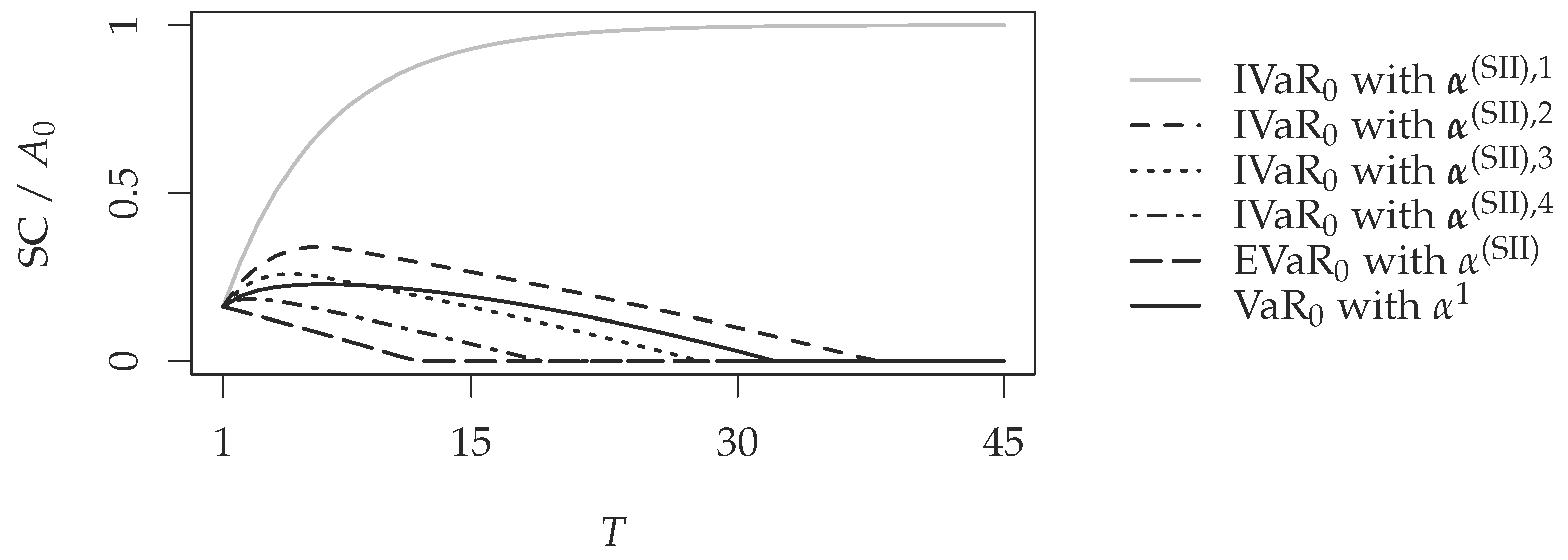
We now study the level of the initial solvency capital according to the previous definitions of the confidence vectors. In Figure 5, we consider the solvency capital at time $t=0$ given by Propositions 3, 4 and 5, for $T\in \{1,\dots ,45\}$ and $K=8$. We only consider the positive part. We observe that for the constant case, i.e., ${\mathit{\alpha }}^{\left(\mathrm{SII}\right),1}$ and ${\mathit{\alpha }}^{\left(\mathrm{SST}\right),1}$, the level of the solvency capital significantly increases with the maturity of the product. As already mentioned, it has been observed in [11,12]. The level of the solvency capital converges towards 100% of the initial value of the portfolio, i.e., towards the present value of the liability, which is here its supremum.

However, for the three others definitions of the confidence level, we remark that the solvency capital level increases for short maturities, while it decreases for long maturities. This decrease in the level is higher when the decrease of the confidence level increases as well, as expected. For instance, the solvency capital under the exponential function ${\mathit{\alpha }}^{\left(\mathrm{SII}\right),4}$ declines more quickly than the solvency capital under the square function ${\mathit{\alpha }}^{\left(\mathrm{SII}\right),3}$. We also observe a similar increasing and decreasing shape with the recalculated VaR and TVaR measures. This shape is very similar to the one given by the maturity approach of [10]. However, the main advantage is that the measure that we consider now is time consistent.

Concerning the EVaR measures, we see that we could consider it as the lower bound for the solvency capital level. This solvency capital is simply the expectation of the solvency capital needed for the last year of the product. It is the best estimate of the capital needed for the last year and does not include any security margin, except for the last year.

The difficulty we face now is the determination of a reasonable or relevant confidence level function. We could obtain any shape of the curve of the solvency capital with a particular choice of the confidence function. A way of solving this would be to consider an easy understandable function, such as the linear increase, e.g., starting K years before the maturity, we increase the confidence level from a fixed amount each year towards a classic level, such as the Solvency II or the Swiss Solvency Test levels.

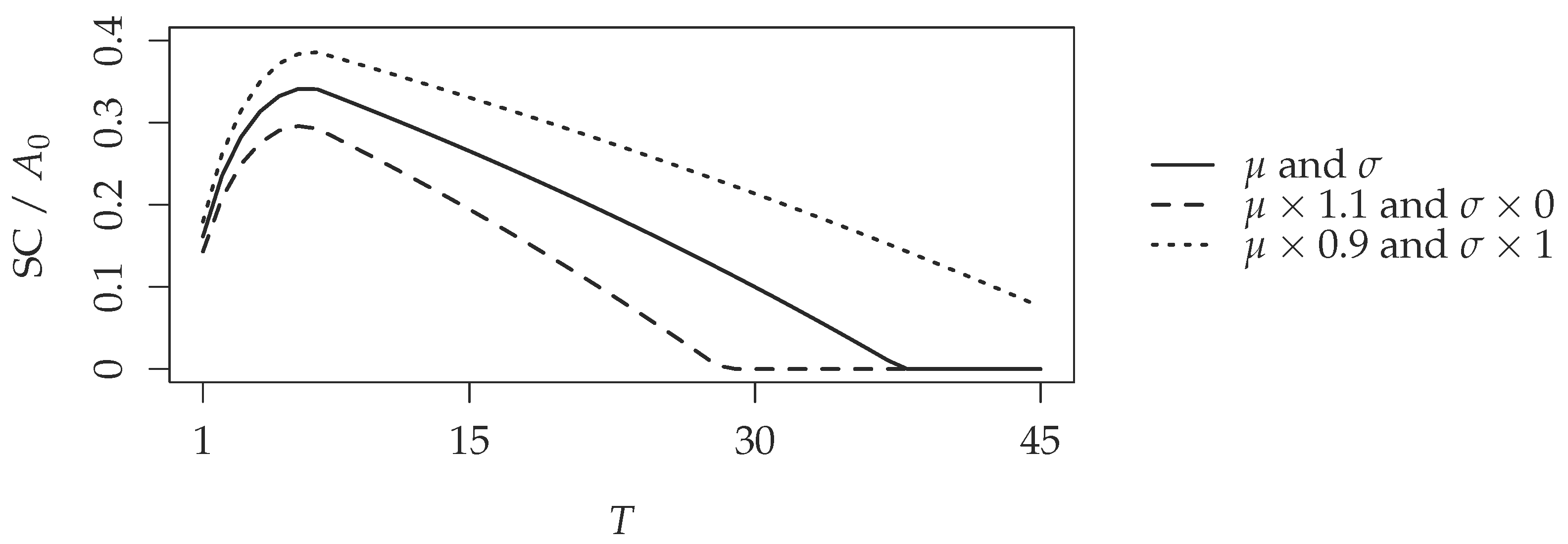
Finally, according to Remark 10, we also observe in Figure 6 that the solvency capital increases when μ decreases and σ increases, while it decreases when μ increases and σ decreases.

8. Conclusions

In this paper, we presented different constructions of time-consistent dynamic risk measures in order to determine the solvency capital of a life insurer or pension fund by taking into account the information disclosed through time. These dynamic risk measures are built such that they are coherent with the Solvency II or Swiss Solvency Test regulatory frameworks in the last year of the product.

We saw that according to the choice of the conditional risk measures considered for the iteration scheme and, in particular, according to the choice of the confidence levels for each iteration, different shapes for the solvency capital can be obtained. Several confidence levels that seem convenient have been proposed in order to benefit from the long-term characteristic of these products.

We also introduced a time-consistent measure where the first iteration is a VaR or TVaR measure, and the subsequent iterations make use of the conditional expectation. This measure is a kind of best estimate of the capital needed for the last year of the product and is particularly intuitive and elegant.

Finally, an important step forward will be to consider the case of multiple cash flows and to include more risks, such as the interest rate and mortality risks.