1. Introduction
The largely unanticipated dynamics of mortality experienced in the latest decades suggests developing new mortality models and to further explore those already known. A critical aspect that we focus on in this paper is understanding how the heterogeneity of the population with respect to mortality does impact on the liabilities of a life annuity provider.
Heterogeneity with respect to mortality can result from observable or non-observable risk factors. While models accounting for observable risk factors generally adopt pragmatic solutions to represent differential mortality (namely, additive or multiplicative adjustments to the average mortality rate), the modeling of heterogeneity due to unobservable risk factors has found an elegant and rigorous solution in the concept of frailty, described already by [
1], but formally defined by [
2]. To some extent, also heterogeneity due to observable risk factors might be represented with a frailty model, via parameter calibration. This could be useful, for instance, when some observable risk factors cannot be adopted as rating factors, as is the case of gender in the EU. In this paper, heterogeneity is addressed via a frailty model. For a short review of models accounting for observable risk factors, see, for example, [
3,
4], as well as the references therein.
Apart from [
1,
2], the impact of heterogeneity on the age-pattern of mortality has been discussed through frailty models by [
5,
6,
7,
8,
9,
10] and many others.
The works in [
1,
2] express the non-observable heterogeneity in terms of a fixed individual frailty level, assuming that the individual frailty is due to genetic factors. Other assumptions have been discussed. The model proposed by [
11] relies on the concept of a frailty that stochastically changes with age, that is throughout the individual life, viz. because of physiological changes and environmental influences. The two approaches are compared by [
12]. Markov aging models, which generalize Le Bras’s assumption, have been adopted by [
13,
14,
15,
16].
The work in [
17] shows that changing frailty models cannot be distinguished from a fixed frailty model. The fixed frailty model is more convenient, especially under the traditional Gompertz-Gamma assumption (see
Section 2). Further, such a model fits satisfactorily a feature observed empirically, but hardly replicated by other models: it provides an analytical justification of the deceleration in the mortality increase at very old ages, observed in many populations.
While frailty models are well known in demography, their application to insurance risk management is not common. Significant research work in the actuarial field is anyhow available. The works in [
18,
19] calibrate (alternatively) two families of frailty models (namely, a Gompertz-Gamma and a Gompertz–Gaussian-inverse model) to insurance-based mortality data, finding evidence of frailty in insured populations. The work in [
20] calibrates the Gompertz-Gamma model to Canadian pensioners’ mortality, finding strong support for the assumption. The work in [
21] analyzes the impact of heterogeneity and frailty on the actuarial values of both standard life annuities and underwritten annuities (i.e., “special rate” life annuities). Conversely, the impact of heterogeneity on tail risk and solvency capital is investigated by [
3,
16].
In this paper, we focus on a potential application of the frailty model, which can be helpful to design a rating system for life annuities arranged in several risk classes.
Risk classification in the area of voluntary life annuities has recently been adopted to stimulate the demand. Indeed, the market is still underdeveloped, as the product is mainly underwritten by healthy people. In order to expand their portfolio, in recent years, some insurers have started offering special annuity rates to those whose health conditions are poor or critical; a useful description of the more common classes of special rate annuities is provided by [
22]. Risk classes can then be identified within a life annuity portfolio, showing different levels of mortality. Adopting models used to represent differential mortality arising from observable risk factors, in common actuarial practice, the higher or lower mortality level of a risk group is represented by applying adjustment coefficients to the population mortality rates. Such coefficients are chosen empirically, calibrated on the average ratio (possibly measured for age groups) between the annuitants’ and the population mortality; conversely, a model formally justifying such a difference is not adopted.
Within a frailty model, lower or higher mortality rates can be explained by lower or higher frailty levels. We then suggest to adopt a frailty model for risk classification. We identify risk groups (or classes) within the population by assigning specific ranges of values to the frailty within each group. Conditional probability distributions for the frailty are obtained for each risk class, which allow us to describe the different levels of mortality of the various groups. Different values for the annuity rate then derive from the different assumptions about the frailty level of the specific risk class.
We also investigate the following issue. When accepting substandard risks, the insurer may increase its portfolio size, but also the heterogeneity of the portfolio. While a larger size implies an improved pooling effect, a higher risk profile follows from the increased heterogeneity. We investigate the result of this trade-off, by assessing the probability distribution of the present value of future benefits. Portfolios with only the standard risk class and with also special rate risk classes are compared, so to measure the trade-off between portfolio size and heterogeneity. We disregard systematic longevity risk, as heterogeneity mainly affects process risk (at least, so long as we can accept that the possible underlying mortality trend is common to all risk groups). We also disregard financial risk, as we mainly focus on the design of a risk classification structure with respect to mortality (and we can exclude a correlation between financial and mortality risk).
The remainder of the paper is arranged as follows. The main features of the traditional frailty model are recalled in
Section 2. In
Section 3, we design a risk classification arrangement for a life annuity portfolio based on a frailty model. In
Section 4, we calibrate the model to Italian projected life tables. In
Section 5, we investigate the probability distribution of the liabilities of life annuity portfolios with different compositions and sizes. Finally,
Section 6 concludes with some further remarks.
2. Lifetime and Frailty: The Gompertz-Gamma Model
The heterogeneity of a population with respect to mortality arises from differences among the individuals. In their seminal paper, [
2] define the frailty as a non-negative quantity whose level expresses the unobservable (and, possibly, some observable) risk factors affecting individual mortality. The underlying idea is that the expected lifetime of individuals with a higher frailty is lower than others. Several models can be developed in this framework; in what follows, we describe the traditional setting. All of the results that are commented on in this section are well known. We then skip the details, which can be found in the references already provided; see, for example, [
2,
19] or [
3].
Refer to a heterogeneous cohort (defined at age 0 and closed to new entrants); in the following, we will use the term population, understanding that it consists of one cohort only. A non-negative, unknown variable called frailty is assigned to each individual, expressing mortality risk factors. The individual frailty level does not change in time, while keeping unknown. Conversely, because of deaths, the average frailty level in the whole population changes with age, and it is expected to decline, given that people with lower frailty are expected to live longer.
Let
denote the force of mortality for an individual current age
x and frailty level
z. The work in [
2] suggests a multiplicative model:
where
, namely the force of mortality for an individual with frailty level
, is called the standard force of mortality (note, however, that in the insurance application,
does not necessarily represent the force of mortality of standard risks; indeed, the class of standard risks can be identified with a frailty interval
, where
can be lower than one, as we discuss in
Section 3.1 and
Section 4). Since the frailty level
z takes the value in
, for the individual force of mortality, we have
. It is worth noting that in (
1), the coefficient
z could be interpreted as a multiplicative adjustment coefficient (with respect to the standard force of mortality), and then,
would represent an adjusted force of mortality. This is to say that Model (
1) resembles the pragmatic approach to differential mortality. However,
z is unknown in (
1), while fixed (and known) adjustment coefficients are adopted in the pragmatic approach. See also the end of
Section 3.1 for a further comment with respect to this comparison.
Denote with
the cumulative standard force of mortality in the age-interval
, i.e.:
The survival function for an individual (newborn) with frailty
z is:
Let
denote the random value of the frailty, whose probability distribution is assessed on the population at age
x and
its probability density function. The average frailty level in the population at age
x is:
while the expected force of mortality of the population at age
x and frailty level
is:
Thanks to the multiplicative assumption (
1), the probability density function of
can easily be derived from
. We find:
where
is the average survival function of the population or the expected share of individuals alive at age
x out of the initial newborns, which can be assessed as follows:
It is interesting to note that only if , and that ; then, the average force of mortality increases less rapidly than the standard one. This is why heterogeneity could explain why the age-pattern of mortality rates shows a deceleration in the increase at the highest ages.
The work in [
2] suggests a Gamma distribution for
, due to its nice features. Then, let
. It can be shown that also
,
, holds a Gamma distribution, with updated parameters; in particular,
. To shorten the notation, we set
, with
; then
for
.
For the average frailty level in the population, we find:
while the variance of
is given by:
Parameters are commonly chosen so that
; thus,
. After noting that the coefficient of variation of
is given by:
we understand that the parameter
δ is chosen considering the degree of heterogeneity of the population. Higher values of
δ corresponds to lower levels of heterogeneity; in particular, the population can be considered (almost) homogeneous when
. Note that, in this model, whilst the expected value of the frailty reduces with age, its relative variability keeps constant.
For the average survival function of the population, we find:
Now, still following [
2], we assume a Gompertz law for the standard force of mortality, namely:
Plugging (
12) and (
8) into (
1), we find the following expression for the average force of mortality of the population:
where:
and
. Equation (
13) shows that the average force of mortality in the population is Perks-type, namely the first Perks law with parameter
; see [
23]. The law (
13) has been proposed also by [
1]; in (
13), the parameters
and
depend on the parameters
of the frailty distribution. We note that (
13) is in the logistic class; such models imply a deceleration in the increasing age-pattern of mortality, which in the current setting is a consequence of the presence of frailty in the population. For a formal approach and more details, see, for example, [
3,
24].
4. Model Calibration
The model described in
Section 3 is general, as it can be applied to any type of life insurance business. In this paper, we discuss the case of immediate life annuities. We refer to a (closed) cohort of males initial age
. We assume that, while group
collects standard risks, higher groups collect preferred risks, i.e. risks with a lower expected lifetime.
The Gompertz-Gamma model is calibrated on Italian projected life tables. In particular, we address the life table TG62, which refers to the general population, and the life table A62I, which is adopted for voluntary immediate life annuities. The projection producing the life table TG62 is performed with the standard Lee–Carter model (see [
25,
26,
27]). Mortality rates for the highest ages (precisely, ages higher than 95) are not based on observed data, but on a parametric model (see [
28]). The life table A62I is obtained by applying reduction coefficients to the mortality rates of the life table TG62. Such coefficients are chosen according to U.K. data and express the self-selection observed in pools of voluntary immediate life annuities (see [
27]). The maximum attainable age in such life tables is
, which we assume also for the Gompertz-Gamma model.
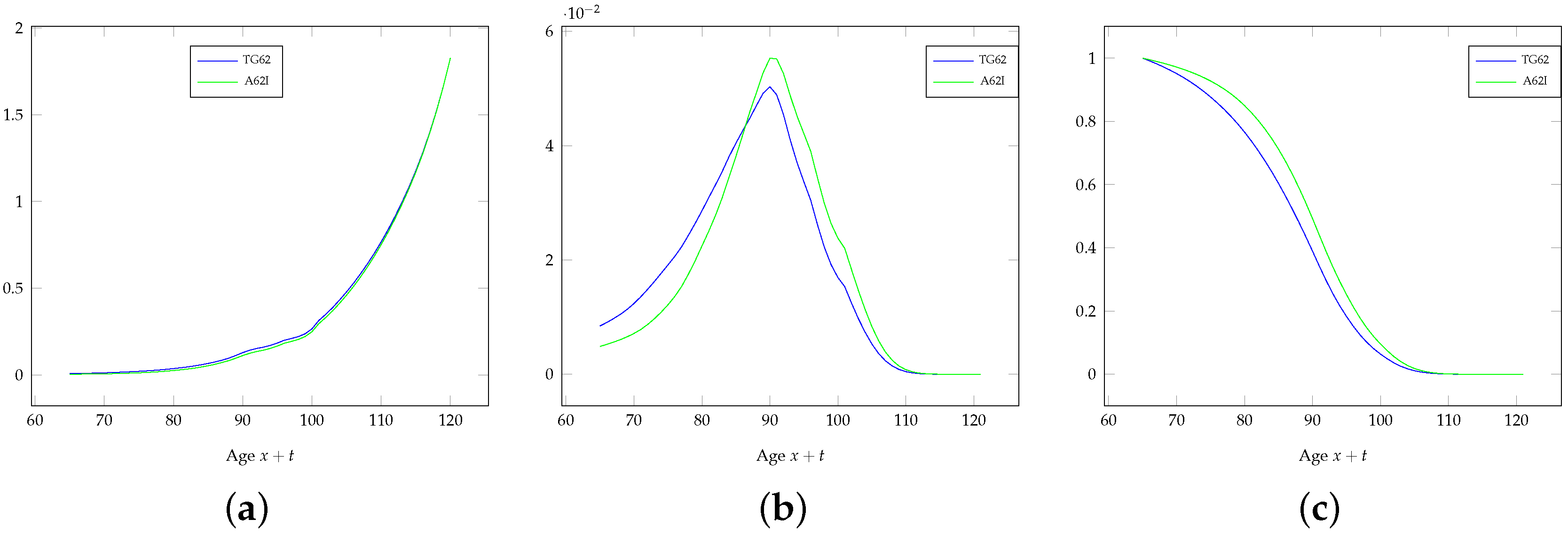
A comparison between the life tables TG62 and A62I is performed in
Figure 1, where the force of mortality, the probability density function of
(i.e., the remaining lifetime at age 65) and the survival function are plotted (the life tables TG62 and A62I list mortality rates and the survival function for integer ages; the force of mortality and the probability density function
have been obtained through standard numerical approximations). The assumed impact of the self-selection of those underwriting a voluntary annuity emerges.
Parameters for the Gompertz-Gamma model are assessed considering only the range of ages
. Higher ages have been disregarded in order to avoid the smoothing effects embedded in the data used for the projection (see above). We perform the following steps.
We first calibrate the mortality model for the general population, based on the life table TG62. As it is common in the literature, we set
; then, we need to set three parameters (namely,
), and we assume the following requirements:
Then, we calibrate the lifetime for standard risks, i.e., individuals in group . We now need to set one parameter (namely, ), and we choose it so to minimize the MSE between the force of mortality under the Gompertz-Gamma model for individuals in group and the table A62I, in the range of ages . Similarly to the life table TG62, the force of mortality for the life table A62I has been approximated numerically. For the Gompertz-Gamma model, the force of mortality for group can be obtained through its definition, as . For simplicity, we omit writing its expression, which cannot be simplified nicely.
Finally, we calibrate the probability distribution of the lifetime for two additional groups, and , characterized by higher average frailty levels; we set a (reasonable) benchmark for the reduced expected lifetime in these groups, with respect to the value for standard risks. Such benchmarks are commented on below.
Table 1 quotes the parameters of the Gompertz-Gamma model for the general population, initial age
. We recall that, since
, we have
, and then,
for
. We note that the heterogeneity measured in the general population is expressed by
. This outcome, which clearly drives the risk classification that we perform, could partially be affected by the modeling assumptions underlying the life table TG62. On the other hand, TG62 is the starting point of the rating of voluntary life annuities in the Italian insurance industry, so we prefer this reference to other choices of the dataset.
Table 2 quotes the summary statistics of the probability distribution of the lifetime
at age 65 for the life table TG62 and for the Gompertz-Gamma model with parameters as in
Table 1. With
, we denote the
ε-percentile of the probability distribution of the lifetime, defined in the usual way;
then denotes the interquartile range, usually meant as a measure of dispersion. There are only small differences between the summary statistics of the probability distribution of
under the life table TG62 and the Gompertz-Gamma model.
Table 3 lists the expected value of the frailty at various ages, as well as the coefficient of variation of the frailty at age
x, which is constant with respect to age (see (
10)).
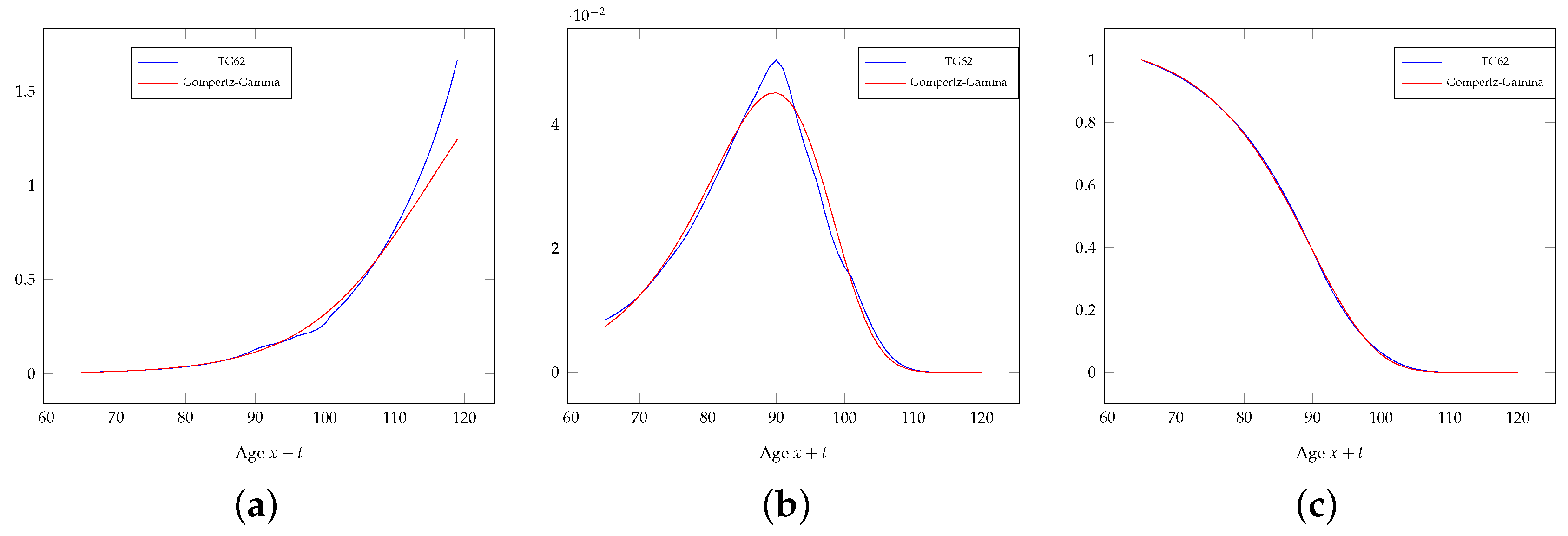
Figure 2 shows the force of mortality, the probability density function of
and the survival function of life table TG62 compared to the Gompertz-Gamma model applied to the general population. The differences between the forces of mortality at the highest ages are due to the different modeling assumptions for this range of ages. Some differences emerge also in the probability density function
; however, when considering the scale of the
y-axis of this plot with respect to the other two, these differences look small.
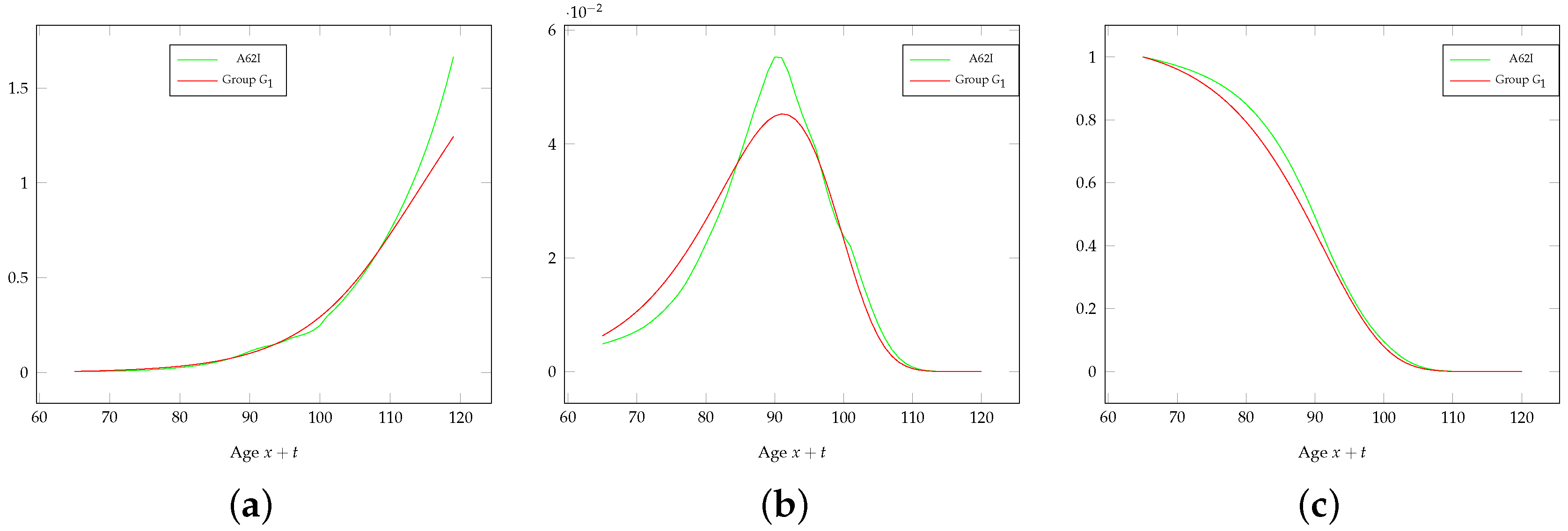
Figure 3 shows the force of mortality, the probability density function of
and the survival function of the life table A62I compared to the Gompertz-Gamma model referring to group
. In this case, some differences are visible also in the survival function; this is due to the very different modeling assumptions about the self-selection backing the life table A62I and the Gompertz-Gamma model. This is confirmed by the comparison between the summary statistics of the probability distribution of
for the life table A62I and the Gompertz-Gamma model for group
, which are quoted in
Table 4. While the method adopted in practice is very pragmatic, the Gompertz-Gamma model leads to a rigorous analytical solution. It is in particular interesting to note that the coefficient of variation of
suggests a wider dispersion of the lifetime for life table A62I than TG62. This is against the idea that the mortality described by A62I refers to a group less heterogeneous than for TG62.
We note here that for setting the parameter , rather than minimizing the MSE between the forces of mortality, we could adopt a requirement involving the expected lifetime (for instance: the same value under A62I and the Gompertz-Gamma model). However, this would lead to unconvincing results about the composition of the population. On the other hand, the life table A62I has been derived from TG62 adjusting the mortality rates; this is also why we set a requirement with respect to the force of mortality.
Table 5 quotes the summary statistics of the frailty at age 65 for the three groups that we identify. The relative size of each group at age 65 refers to the general population; the real composition of the insurer’s portfolio depends on the number of people actually underwriting the contract. Note that each risk class shows a reduced coefficient of variation of the frailty (and then, less heterogeneity) with respect to the general population, as well as a lower (namely, group
) or higher (namely, groups
and
) average frailty level. Note also that we have assumed that the expected lifetime of those in group
is 12% higher than those in group
and roughly 22% higher than those in group
. We think that these assumptions are reasonable with respect to the available data. Of course, different choices are possible. One could decide to set just one additional risk class for special rate annuities or more than two classes; further, different values for the lower expected lifetime for those in higher classes could be set. The final choice depends on what is classified as a critical health condition, how the health status can be ascertained, as well as on market issues.
6. Some Remarks to Conclude
This paper is mainly motivated by the need to model differential mortality for life annuities, following the introduction of special rate annuities. The solution adopted in current actuarial practice is pragmatic and straightforward to implement, but is not completely satisfactory, as it is not backed by a rigorous model. The Gompertz-Gamma model that we adopt in this paper is simple, but is convenient, in particular in view of practical applications. We show how it could be implemented to realize a rigorous rating system arranged in risk classes. In any case, it can be adopted for estimating the potential composition of a heterogeneous portfolio.
Further, we investigate the impact on the insurer’s liabilities of the increased portfolio heterogeneity following the introduction of special rate annuities. As is known, higher degrees of heterogeneity imply a higher risk profile for the provider. However, if matched by a larger portfolio size, the risk profile of the insurer can benefit from a portfolio diversification (clearly, if appropriate annuity rates are adopted). Indeed, the higher volatility incurred because of the portfolio heterogeneity is more than compensated by the stronger pooling effect resulting from the larger size. The specific choice of the rating structure seems to have a significant impact on the expected value of insurer’s liabilities, rather than on its risk profile.
Various directions for future research can be conceived. First, we note that adverse-selection could emerge as a result of the rating structure, and its possible impact should be addressed, possibly through a modeling of the demand, which represents a possible topic for future research.
A further aspect that is interesting to investigate is the impact on insurer’s liabilities of an incorrect allocation of risks to the various risk classes. Since the frailty is unobservable and the risk classification is based on observable proxies, a misspecification of the risk class is always possible. This would result in an unfair annuity rate applied to some individuals and then in an increased (or reduced) probability of loss for the insurer. In this regard, the research task concerns in particular the modeling of the incorrect specification of the risk class.
In the paper, we have assumed that insurer’s liabilities are only affected by the volatility caused by random fluctuations in mortality and frailty. However, a major risk for a life annuity provider is the aggregate longevity risk, namely the risk of unanticipated mortality improvements. It is reasonable, in particular, to assume that the several risk groups follow different mortality trends, anyhow correlated (in particular because of the underlying frailty distribution). While the joint modeling of the frailty and the stochastic mortality dynamics is controversial, this is a research topic that should be further developed.


