Nested MC-Based Risk Measurement of Complex Portfolios: Acceleration and Energy Efficiency

Abstract

Risk analysis and management currently have a strong presence in financial institutions, where high performance and energy efficiency are key requirements for acceleration systems, especially when it comes to intraday analysis. In this regard, we approach the estimation of the widely-employed portfolio risk metrics value-at-risk (VaR) and conditional value-at-risk (cVaR) by means of nested Monte Carlo (MC) simulations. We do so by combining theory and software/hardware implementation. This allows us for the first time to investigate their performance on heterogeneous compute systems and across different compute platforms, namely central processing unit (CPU), many integrated core (MIC) architecture XeonPhi, graphics processing unit (GPU), and field-programmable gate array (FPGA). To this end, the OpenCL framework is employed to generate portable code, and the size of the simulations is scaled in order to evaluate variations in performance. Furthermore, we assess different parallelization schemes, and the targeted platforms are evaluated and compared in terms of runtime and energy efficiency. Our implementation also allowed us to derive a new algorithmic optimization regarding the generation of the required random number sequences. Moreover, we provide specific guidelines on how to properly handle these sequences in portable code, and on how to efficiently implement nested MC-based VaR and cVaR simulations on heterogeneous compute systems.

1. Introduction

Risk metrics are traditionally computed overnight on large compute clusters, due to the extended runtime and complexity, which highlights the need for efficient acceleration. The importance of those metrics in practice is for instance underlined by JPmMorgan’s famous technical document [1], which is still in use today. When it comes to large portfolios including complex path-dependent nonlinear derivatives, the most appropriate method for the calculation of risk measures such as the value-at-risk (VaR) and the conditional value-at-risk (cVaR) is Monte Carlo (MC) simulation (compare, e.g., [2]). A major reason for this is that analytical approximations such as the delta-gamma method are often too inaccurate in such a setting.

In this paper, we focus on the efficient computation of the VaR and cVaR of a stylized portfolio containing derivatives with nonlinear payoffs that require MC simulation for the pricing of the derivative (the so-called inner simulation) and for the calculation of the empirical distribution function in order to determine the quantile of the loss distribution based on risk factors (the so called outer simulation). The MC evaluation of such complex portfolios thus leads to nested simulations, which have been extensively studied by Gordy and Juneja in [3] from a mathematical point of view. In particular, they show that these nested schemes involve a serious computational burden.

These computationally-intense problems in finance face a serious interest in high-performance computing, especially on heterogeneous compute clusters composed of different processing units, such as central processing unit (CPU), graphics processor unit (GPU), and field programmable gate array (FPGA). This is reflected by a large amount of corresponding literature. For instance, in the context of credit risk, Rees and Walkenhorst have achieved around 90× runtime acceleration on a GPU [4], while Thomas and Luk have shown a 60–100× runtime acceleration on a FPGA [5], both compared to a CPU. Concerning interest rate theory, Albanese has shown in [6] the usefulness of parallel GPU architectures for the pricing of complex interest rate derivatives.

Closer to the analysis of this paper, there is a strand of literature focusing on the hardware efficient computation of a portfolio-based VaR. Dixon et al. have implemented a MC-based delta-gamma VaR approximation on GPUs, focusing on three different perspectives: task-, numerical-, and data-centric [7]. In this way, they have shown up to 169× runtime acceleration compared to a baseline GPU implementation, all programmed in Compute Unified Device Architecture (CUDA) [8]. Zhang et al. have also evaluated the delta-gamma approach for the computation of the VaR with GPUs using Open Compute Language (OpenCL) [9]. However, in both cases, the MC-approach is only used for the outer simulation, whereas the pricing within the inner simulation was performed using a delta-gamma approximation of the loss function. On architecturally diverse systems, Singla et al. have proposed different mappings of the MC-based portfolio VaR, achieving a 74× speedup relative to an eight-core CPU processor [10]. Their results show two winning solutions for the mapping of the MC simulation: a full GPU implementation, and the pair FPGA–CPU and GPU working in parallel, for which they hint at the design complexity. Nevertheless, their work only targeted a simple stock-based portfolio using the Black-Scholes (BS) model, thus preventing nested simulations.

Our work focuses on nested MC simulations, as in [3] in order to determine a VaR as well as a cVaR on portfolio level, further expanding our preliminary results in [11]. This approach allows for the implementation of mathematical models with a high complexity and for the pricing of derivatives with a highly nonlinear payoff. For that sake, we have defined a representative portfolio consisting of cash, stocks, bonds, options, and foreign currency with a corresponding set of market parameters, and the derived results are valid within the framework of these selected parameters.

The nested MC simulations are an ideal candidate for hardware acceleration, and as such, we target in particular heterogeneous compute systems, including CPU, XeonPhi, GPU, and FPGA platforms. Although generic and well-known benchmarks (such as 3DMark [12]) could be used to profile the performance of the targeted hardware, here we demonstrate and assess how to efficiently map these nested MC simulations onto such heterogenous compute systems. In this regard, we solve the design complexity by exploiting the portability offered by OpenCL, which enables us to quickly deploy the code to multiple platforms, increasing productivity. Furthermore, we analyze the portability of our work, and we also highlight key aspects that the programmer must bear in mind when moving the project between platforms.

The nested VaR and cVaR calculation can also be parallelized. To this end, we assess the pros and cons of three different parallelization schemes, and we highlight the most suitable one for the given platforms. One aspect that we cover is the proper handling of the random number (RN) sequences, especially within portable code. In our case we employ the Mersenne twister (MT) pseudo random number generator (PRNG). Not only the correct setup of the generators is important, but the code should also carefully access the RN sequences in the same order on different platforms. At system level, we present an algorithmic optimization, namely the external generation of the RN sequences, and we evaluate its effect on the speedup experienced on every platform, including an assessment of the asymptotic time and space complexity. We also provide extensive simulations and data for a detailed comparison of all four platforms in terms of runtime and energy consumption, and comment on the achieved performances.

2. Basics of Market Risk Quantification: VaR and cVaR

When quantifying market risks, we are particularly interested in the potential losses of the total value of the portfolio over a future time period. The appropriate concepts for measuring the risk of such a portfolio of financial assets are those of the loss function and of risk measures. We will be quite brief on these basics and refer to the corresponding sections of [13] and [14] for more details.

We denote the value at time s of the portfolio under consideration by $V\left(s\right)$ and assume that the random variable $V\left(s\right)$ is observable at time s. Further, we assume that the composition of the portfolio does not change over the period we are looking at.

For a time horizon of Δ, the portfolio loss over the period $[s,s+\Delta ]$ is given by

$$\begin{array}{c}\hfill L_{[s,s+\Delta ]}\triangleq -\left(V(s+\Delta )-V\left(s\right)\right).\end{array}$$

As $L_{[s,s+\Delta ]}$ is not known at time s, it is considered to be a random variable. Its distribution is called the (portfolio) loss distribution.

As in [13], we will work in units of the fixed time horizon Δ, introduce the notation $V_t\triangleq V(t\Delta )$, and rewrite the loss function as

$$\begin{array}{c}\hfill L_{t+1}\triangleq L_{[t\Delta ,(t+1)\Delta ]}=-(V_{t+1}-V_t).\end{array}$$

(1)

Fixing the time t, the distribution of the loss function $L\triangleq L_{t+1}$ for $\ell \in \mathbb{R}$ (conditional on time t) is introduced using a simplified notation as

$$\begin{array}{c}\hfill F_L\left(\ell \right)\triangleq P(L\le \ell ).\end{array}$$

We now introduce a risk measure ρ as a real-valued mapping defined on the space of random variables which correspond to the risks that are faced.

There exists a huge amount of different risk measures which all have certain advantages and drawbacks, but the most popular example of a risk measure which is mainly used in banks (and which has become an industry standard) is still the value-at-risk (VaR). It is defined as follows:

The value-at-risk of level α ($Va{R}_{\alpha }$) is the α-quantile of the loss distribution of the portfolio; i.e.,

$$\begin{array}{c}\hfill Va{R}_{\alpha }\left(L\right)\triangleq \underset{\ell \in \mathbb{R}}{inf}\left\{P(L>\ell )\le 1-\alpha \right\}=\underset{\ell \in \mathbb{R}}{inf}\left\{F_L\left(\ell \right)\ge \alpha \right\},\end{array}$$

where α is a high percentage, such as $95\%$, $99\%$, or $99.5\%$.

By its nature as a quantile, the values of $Va{R}_{\alpha }$ have an understandable meaning, a fact that makes it very popular in a wide range of applications, mainly for the measurement of market risks. The value-at-risk is not necessarily sub-additive; i.e., it is possible that $Va{R}_{\alpha }(X+Y)>Va{R}_{\alpha }\left(X\right)+Va{R}_{\alpha }\left(Y\right)$ for two different risks $X,Y$. This drawback is the basis for most of the criticism of using value-at-risk as a risk measure. Furthermore, as a quantile, $Va{R}_{\alpha }$ does not say anything about the actual losses above it.

A risk measure that does not suffer from these two drawbacks—and which is therefore also popular in applications—is the conditional value-at-risk (cVaR), and is defined as

$$\begin{array}{c}\hfill cVa{R}_{\alpha }\left(L\right)\triangleq \frac{1}{1-\alpha }{\int }_{\alpha }^{1}Va{R}_{\gamma }\left(L\right)\mathrm{d}\gamma .\end{array}$$

If the probability distribution of L has no atoms, then the $cVa{R}_{\alpha }$ has the interpretation as the expected losses above the value-at-risk; i.e., it then coincides with the expected shortfall or tail conditional expectation defined by

$$\begin{array}{c}\hfill TC{E}_{\alpha }\left(L\right)\triangleq \mathbb{E}\left(L|L\le Va{R}_{\alpha }\left(L\right)\right).\end{array}$$

As the conditional value-at-risk is the value at risk integrated w.r.t. the confidence level, both notions do not differ greatly from the computational point of view. In particular, once we have the loss distribution, the VaR and cVaR computation is straight-forward, which is also underlined by our numerical investigations.

However, as typically the portfolio value V (and thus by (1) the loss function L) depend on a d-dimensional vector of market prices for a very large dimension d, the loss function will depend on the market prices of maybe thousands of different derivative securities.

The first step to making a large portfolio tractable is to introduce risk factors that can explain (most of) the variations of the loss function, and ideally reduce the dimension of the problem. These risk factors can be, for instance, log-returns of stocks, indices, or economic indicators, or a combination of them. A classical method for performing such a model reduction and for finding risk factors is a principal component analysis of the returns of the underlying positions.

We do not go further here, but simply assume that the portfolio value is modeled by a risk mapping; i.e., for a d-dimensional random vector ${\mathbf{Z}}_t\triangleq {(Z_{t,1},\dots ,Z_{t,d})}^{\prime }$ of risk factors, we have the representation

$$\begin{array}{c}\hfill V_t=f(t,{\mathbf{Z}}_t)\end{array}$$

(2)

for some measurable function $f:{\mathbb{R}}_{+}\times {\mathbb{R}}^d\to \mathbb{R}$. By introducing the risk factor changes ${\left({\mathbf{X}}_t\right)}_{t\in \mathbb{N}}$ by ${\mathbf{X}}_t\triangleq {\mathbf{Z}}_t-{\mathbf{Z}}_{t-1}$, the portfolio loss can be written as

$$\begin{array}{ccc}\hfill L_{t+1}\left(X_{t+1}\right)& =& -\left(f(t+1,{\mathbf{Z}}_t+{\mathbf{X}}_{t+1})-f(t,{\mathbf{Z}}_t)\right)\hfill \end{array}$$

(3)

highlighting that the loss is completely determined by the risk factor changes.

With the representations (2) and (3), we are now able to detail how the MC method is used for the quantification of market risks.

2.1. The MC Method

The MC method assumes a certain distribution of the future risk factor changes; e.g., we can suppose but are not limited to a Black–Scholes model or a Heston model, as we do it for the upcoming analysis. Once the choice of this distribution has been made, the MC method simulates independent identically distributed random future risk factor changes ${\tilde{\mathbf{X}}}_{t+1}^{\left(1\right)},\dots ,{\tilde{\mathbf{X}}}_{t+1}^{\left(M\right)}$, and then computes the corresponding portfolio losses

$$\begin{array}{c}\hfill \left\{{\tilde{L}}_{t+1}({\tilde{\mathbf{X}}}_{t+1}^{\left(i\right)}):i=1,\dots ,M\right\}.\end{array}$$

(4)

Based on these simulated loss data, one now estimates the value-at-risk by the corresponding empirical quantile; i.e., the quantile of the obtained simulated empirical loss distribution:

The MC estimator for the value-at-risk is given by

$$\begin{array}{c}\hfill Va{R}_{\alpha }({\tilde{L}}_{t+1})\triangleq \underset{\ell \in \mathbb{R}}{inf}\left\{{\tilde{F}}_{t+1}\left(\ell \right)\ge \alpha \right\},\end{array}$$

where the empirical distribution function ${\tilde{F}}_{t+1}\left(\ell \right)$ is given by

$$\begin{array}{c}\hfill {\tilde{F}}_{t+1}\left(\ell \right)\triangleq \frac{1}{M}\sum _{i=1}^M{I}_{\{{\tilde{L}}_{t+1}({\tilde{\mathbf{X}}}_{t+1}^{\left(i\right)})\le \ell \}}.\end{array}$$

The MC estimator for the conditional value-at-risk is given by its empirical counterpart

$$\begin{array}{c}\hfill cVa{R}_{\alpha }({\tilde{L}}_{t+1})\triangleq \frac{1}{1-\alpha }{\int }_{\alpha }^{1}Va{R}_{\gamma }({\tilde{L}}_{t+1})\mathrm{d}\gamma .\end{array}$$

The above simulation to generate the risk factor changes is often named the outer simulation. Depending on the complexity of the derivatives included in the portfolio, we will need an inner simulation in order to evaluate the loss function of the risk factor changes.

More precisely, whenever our portfolio contains derivatives that do not admit a closed-form pricing formula, we have to calculate their prices by a numerical method. In our case, we choose MC simulation as this method. Thus, we have to perform MC simulations to calculate the future values of options in each run of the outer simulation.

2.2. The MC Method: Nested Simulations

As already pointed out, in the MC method we have to evaluate the portfolio in its full complexity. This computational challenge is carried to extremes when the portfolio contains derivatives without a closed-form price representation. We then need the announced inner MC simulation in addition to the outer one to compute each realized loss value.

To formalize this, assume for notational convenience that the time horizon Δ is fixed, that time $t+1$ corresponds to time $t+\Delta$, and that the risk mapping $f:{\mathbb{R}}_{+}\times {\mathbb{R}}^d\to \mathbb{R}$ corresponds to a portfolio of derivatives with payoff functions $H_1,\dots ,H_K$ with maturities $T_1,\dots ,T_K$. Thus, with $\tilde{\mathbb{E}}(.)$ denoting the expectation under the risk neutral measure Q, the risk mapping f at time $t+\Delta$ is given by

$$\begin{array}{c}\hfill f(t+\Delta ,{\mathbf{Z}}_t+{\tilde{\mathbf{X}}}_{t+\Delta }^{\left(i\right)})=\sum _{k=1}^K\tilde{\mathbb{E}}\left[e^{-r(T_k-(t+\Delta ))}{H}_k|{\tilde{\mathbf{X}}}_{t+\Delta }^{\left(i\right)}\right];\end{array}$$

(5)

i.e.,

$$\begin{array}{c}\hfill {\tilde{L}}_{t+\Delta }({\tilde{\mathbf{X}}}_{t+\Delta }^{\left(i\right)})\triangleq -\left(\sum _{k=1}^K\tilde{\mathbb{E}}\left[e^{-r(T_k-(t+\Delta ))}{H}_k|{\tilde{\mathbf{X}}}_{t+\Delta }^{\left(i\right)}\right]-f(t,{\mathbf{Z}}_t)\right).\end{array}$$

(6)

For standard derivatives like European calls or puts, the conditional expectations can be computed in closed-form. For complex derivatives, however, they have to be determined via MC simulation. The algorithm that describes the inner MC simulation for complex derivatives in the portfolio is given by:

• Generate $N$ independent realizations $H_k^{\left(1\right)},\dots ,H_k^{\left(N\right)}$ of the $k=1,\dots ,K$ (complex) payoffs given ${\tilde{\mathbf{X}}}_{t+\Delta }^{\left(i\right)}$.
• Estimate the discounted conditional expectation of the payoff functions by

  $$\begin{array}{c}\hfill \tilde{\mathbb{E}}\left[e^{-r(T_k-(t+\Delta ))}{H}_k|{\tilde{\mathbf{X}}}_{t+\Delta }^{\left(i\right)}\right]\approx \frac{e^{-r(T_k-(t+\Delta ))}}{N}\sum _{j=1}^N{H}_k^{\left(j\right)}({\tilde{\mathbf{X}}}_{t+\Delta }^{\left(i\right)})\end{array}$$

  for $k=1,\dots ,K$.

It is important to understand correctly that $H_k^{\left(j\right)}({\tilde{\mathbf{X}}}_{t+\Delta }^{\left(i\right)})$ denotes a realization of the payoff of the $k^{th}$ derivative conditioned on the input value ${\tilde{\mathbf{X}}}_{t+\Delta }^{\left(i\right)}$. An example of that can be the payoff of a call option on $X_{t+2\Delta }$, conditioned on the X-value of ${\tilde{\mathbf{X}}}_{t+\Delta }^{\left(i\right)}$ at time $t+\Delta$.

Thus, the MC estimator for the value-at-risk of a complex portfolio is given by

$$\begin{array}{c}\hfill Va{R}_{\alpha }({\tilde{L}}_{t+1})\triangleq inf\{x\in \mathbb{R}|{\tilde{F}}_{t+1}\left(x\right)\ge \alpha \},\end{array}$$

(7)

where the empirical distribution function ${\tilde{F}}_{t+1}\left(x\right)$ is given by

$$\begin{array}{c}\hfill {\tilde{F}}_{t+1}\left(x\right)\triangleq \frac{1}{M}\sum _{i=1}^M{I}_{\{{\tilde{L}}_{t+1}({\tilde{\mathbf{X}}}_{t+1}^{\left(i\right)})\le x\}},\end{array}$$

(8)

and the portfolio losses are given by

$$\begin{array}{c}\hfill {\tilde{L}}_{t+1}({\tilde{\mathbf{X}}}_{t+1}^{\left(i\right)})\triangleq -\left(\sum _{k=1}^K\left(\frac{e^{-r(T_k-(t+1))}}{N}\sum _{j=1}^N{H}_k^{\left(j\right)}({\tilde{\mathbf{X}}}_{t+1}^{\left(i\right)})\right)-f(t,{\mathbf{Z}}_t)\right).\end{array}$$

(9)

Again, the MC estimator for the conditional value-at-risk is given by its empirical counterpart

$$\begin{array}{c}\hfill cVa{R}_{\alpha }({\tilde{L}}_{t+1})\triangleq \frac{1}{1-\alpha }{\int }_{\alpha }^{1}Va{R}_{\gamma }({\tilde{L}}_{t+1})\mathrm{d}\gamma .\end{array}$$

(10)

The amount of simulation work in the presence of the need for an inner simulation is enormous, as the inner simulations have to be redone for each run of the outer simulation. Given a finite computation time, balancing the load between inner and outer simulation while computing the VaR resp. cVaR with an adequate accuracy is a serious issue. Highly accurate derivative prices in the inner simulation lead to an accurate evaluation of the loss function. On the other hand, they cause a big computational effort, which then results in the possibility of performing only a few outer simulation runs. This then leads to a poor estimate of the VaR/cVaR value. A high number of outer simulation runs, however, only allows for a very rough estimation of the derivative prices on the inner run; again, a non-desirable effect. Therefore, it is essential to balance the number of inner and outer simulations. For further details on this computational challenge, we refer the reader to [15].

This behavior is also illustrated in Figure 1, where we consider a very simple portfolio consisting of just one option maturing at the end of the year. The figure shows three simulations under the subjective measure P of the outer paths, resulting in the three values of the underlying stock price at (for example) mid-February. To obtain the resulting portfolio value (i.e., the option price) at mid-February given the just-simulated stock price, one then has to simulate a large number of stock price paths until the end of the year under Q, of course each one starting at the mid-February price.

3. Portfolio Risk Setup

The composition of a portfolio is tailor-made to the investment strategy of the financial institution or even to the individual requirements of each client. Financial products typically found in portfolios are, for example, stocks, bonds, options, foreign currency, or cash (to keep a certain liquidity level). From a computational point of view, pricing the complete portfolio is a highly heterogeneous problem, since each product has its own pricing algorithm with its own associated complexity.

For our stylized exemplary portfolio, we assume from now on that the risk mapping (3) has been predetermined. We also assume that all parameters of the models used for the simulation of the risk factor changes (outer simulation) and for the simulation of the dynamics of the complex derivatives (inner simulation) have been predetermined. For this paper, we focus on the speed-up when considering nested simulations (see Section 2.2) that arise when the MC approach is used for both the outer and the inner simulation. Both simulations are performed either with the BS or the Heston model. In this test-case, this applies to the correlated stocks and the European style options.

The chosen representative portfolio composition is presented in

Table 1. Portfolio composition.

Products		Portfolio	Maturity	Characteristics	Simulation
Group	Description	Weight	(Years)
Stocks	Stock A	15%	-	long position	MC
	Stock B	15%	-	long position	MC
Bonds	Corporate Bond	30%	10.0	annual coupons	MC
Options	European Asian	5%	1.0	on stock 1	MC
	European Barrier	5%	1.0	on stock 2	MC
	American Vanilla	5%	1.0	on stock 1	BT
Cash	Dollar	10%	-	-	-
Cross Currency	Euro/Dollar	15%	-	long position	MC

, which shows the potential of the nested MC simulation, in particular for complex derivatives. The latter have been selected according to their computational complexity, as a representative sample of commonly traded options. American option pricing is a computationally intensive problem, which can be solved, for example, by applying a Binomial Tree (BT) method [16], or the MC-based Longstaff-Schwartz (LS) algorithm in particular for the multi-dimensional case [17,18]. Since in our test-case portfolio we deal with the one-dimensional case, the former is chosen due to its simplicity and lower runtime. Barrier options are frequently traded and require (at least) fine-grained steps to cope with the computational complexity close to the barrier [19]. Asian options are less computationally intensive, but still require a MC approach [19].

The VaR and cVaR on portfolio level are calculated using Equations (7)–(10) by aggregating the loss functions of the different portfolio ingredients, as given in Table 1. This means in particular that we directly calculate the VaR of the total loss and do not aggregate the VaR of the single positions. Thus, we do not need the questionable assumption of additivity of the VaR of single positions (compare Section 2).

3.1. Nested MC-Based VaR and cVaR Setup

Below, we list the main parameters that are used throughout the coming sections if not stated otherwise:

• VaR/cVaR days       : 1
• VaR/cVaR prob.      : 0.99 (${\alpha }_{quantile}=0.01$)
• pathsMCext          : 32k (where $1k\triangleq 1024$)
• pathsMCint          : 32k (where $1k\triangleq 1024$)
• stepsMCext          : 1 for BS, 4 for Heston
• Options Maturity   : 1 year (assuming 252 trading days)
• stepsMCint          : 252 for European Asian, 1008 (= 252*4) for European Barrier
• stepsTree             : 252 (= pathsMCint)

The number of MC paths, both external (pathsMCext) and internal (pathsMCint), is thereby chosen as 32k. This prevents us from facing the problem of too few simulations, while keeping the numerical complexity tractable.

3.2. Computational Complexity

Figure 2 shows the (preliminary) runtime percentages of a full VaR/VaR computation for the portfolio given in Table 1, coded in Matlab (optimized). From these results, it is evident that the major part of the computational complexity originates when highly non-linear derivatives have to be priced within the inner MC simulation. Note that in the case of high-dimensional options, the BT method becomes impractical for the American Vanilla (both in terms of runtime and implementation), in which case the LS algorithm is preferred. In such a case, the computational complexity of this kernel becomes relevant. For example, if our portfolio included an American 2D Max call option, the runtime distribution would be: European Barrier: $64\%$, American 2D Max: $22\%$, and European Asian $13\%$ approximately [11].

3.3. Hardware Setup

The hardware setup of our high-performance workstation is detailed below:

• SuperMicro Superserver 7048GR-TR (with a dual-socket X10DRG-Q motherboard, 2000 W Titanium level high-efficiency redundant power supplies, and the required cooling kit MCP-320-74701-0N-KIT) [22,23].
• (2×) Intel Xeon Processor E5-2670V3 (Haswell architecture, 12 cores (24 threads) @ 2.3 GHz base frequency, (8×) 8 GB DDR4). Technology node: 22 nm [24].
• (1×) Intel Xeon Phi Coprocessor 7120P (61 cores @ 1.238 GHz base frequency, 16 GB, passive cooling). Technology node: 22 nm [25].
• (×1) Nvidia Tesla K80 GPU Accelerator (with dual GK210 GPU, (2×) 2596 CUDA Cores @ 560 MHz base frequency, (2×) 12 GB, passive cooling). Technology node: 28 nm [26,27].
• (×1) Alpha Data ADM-PCIE-7V3 (with Xilinx Virtex-7 FPGA model XC7VX690T-2 (FFG1157C), 200 MHz SDAccel frequency, 16 GB, active cooling (small fan). Technology node: 28 nm [28].

Our workstation operates with Linux RedHat 6.6 (Linux 2.6.32-504.el6.x86_64), and all individual OpenCL drivers and additional software were installed from scratch.

Four Host+Accelerator combinations are evaluated in this work: CPU+CPU (exploiting the dual-socket X10DRG-Q motherboard), CPU+XeonPhi, CPU+GPU, and CPU+FPGA.

The FPGA card has also been installed and measured used on a much smaller system setup (PC) with an MSI B85M-E45 motherboard [20], Intel Core I7-4970 (Technology node: 22 nm) [21], 16 GB DDR3 memory, running CentOS 6.7 (2.6.32-573.18.1.el6.x86_64).

Throughout this work, the room temperature is controlled at ∼23 ${}^{\circ }$C.

Notes on Technology Node Differences

In the above description of our main workstation, the term technology node refers to the minimum size of features in the underlying semiconductor technology. Ideally, platforms should be compared at the same technology node, since smaller (newer) ones confer (in general terms) higher performance and energy efficiency (for details on the effects of technology scaling, refer to [29]). However, this is not always possible, since it is vendor dependent. Therefore, we can still compare the four platforms, as long as these differences are accounted for.

3.4. Relevant Platform Characteristics: CPU, XeonPhi, GPU, and FPGA

A summary of the most relevant characteristics for this work are detailed below:

• CPU: The most general and versatile platform. It is usually preferred to add an accelerator device to offload time-consuming computations. The Intel Xeon processor is mainly designed to have a good performance per single core/thread, while offering a moderate number of parallel cores [30,31].
• XeonPhi: It is a many integrated core (MIC) architecture offered by Intel for acceleration purposes. Each core includes a 512-bit vector arithmetic unit capable of executing wide single instruction multiple data (SIMD) instructions [31,32]. Code that runs on Xeon processors should be slightly modified to run on these devices, and Intel provides development environments for that purpose (in our case, we focus on portable OpenCL). One detail to always bear in mind when using the XeonPhi is that there is no barrier synchronization support in hardware for the work items in the same work group, which is currently simulated in software [32]. After extensive tests, the ideal work group size turned out to be around 16 work items, exploiting the implicit vectorization module. Several tests we have carried out have shown that it is possible to avoid hardware synchronization completely when using a work group size equal to the size of the vectorization module, a finding that is exploited in the rest of our work.
• GPU: This device was originally designed for image rendering purposes, offloading these tasks from the CPU. Over time, GPUs have become widely used for general purpose computations and have evolved into extremely efficient devices. They rely on executing many parallel threads (work items in OpenCL) on many processor cores. These cores are simple but highly optimized for data-parallel computations among groups of threads [33]. As a general rule, the larger the work group size (currently around 1024 work items) and the larger the number of work groups, the better the device is exploited; i.e., for light workloads, it will be underutilized.
• FPGA: Besides the details mentioned in Section 4.2, the key strengths of FPGAs can be summarized in four points:

  -

  Pipelining: The for-loops that are pipelined resemble an assembly line in a manufacturing company, where products go from one station to the next, each performing a set of specific operations. Assembly lines are optimized so that multiple items are on the line simultaneously, and no station is idle at any point in time. Similarly, for-loops that are pipelined can start processing a new input (or iteration) before the output for the current input (iteration) is ready. The most efficient for-loops are those whose initiation interval—the time needed between two consecutive inputs—is just one clock cycle.

  -

  Infinite bit-level parallelism: Being a customized architecture, parallelism can be widely exploited, even at bit level.

  -

  Customized precision: FPGAs are not restricted to fixed data types, which means that custom precision data types can be exploited (although not in this work).

  -

  Customized memory hierarchy: Because of the available on-device random access memory (RAM), accessed faster than external global memory, the architecture can efficiently exploit a tailor-made memory hierarchy.

The key with FPGAs is to obtain a pipelined architecture with an initiation interval of one clock cycle. After a certain latency, the first output will be available, and from that point onward there will be an output value in every consecutive clock cycle. Furthermore, these pipelines usually need to be wide, computing as many numbers in parallel as possible, and expanding the architecture to use as many FPGA resources as possible.

4. OpenCL

No single platform can efficiently cope with all classes of workloads, and most applications include a variety of workload characteristics. Therefore, systems are designed today based on heterogeneous compute systems. This provides the programmer with enough flexibility to choose the best architecture for the given task, or to select the task that optimally exploits the given platform. However, this flexibility comes at the expense of an increased programming complexity [34].

OpenCL is an open, royalty-free standard for general purpose parallel programming that can be ported to multiple platforms, including CPUs, GPUs, and FPGAs. OpenCL is managed by the Khronos Group, a nonprofit technology consortium. It basically utilizes a subset of ISO C99 with extensions for parallelism, and it supports both data- and task-based parallel programming models [35]. The main idea behind this framework is to allow the development of portable code across different platforms, reducing the programming effort when it comes to heterogeneous systems.

There are, however, three key aspects that need to be highlighted. First, although OpenCL code is portable, its performance is not necessarily so, which means that the same code still needs to be optimized for the targeted platform in order to achieve a high efficiency. Second, a somewhat higher performance should be expected from platform-specific programming frameworks, such as CUDA on GPUs (see as examples [11,36]). Third, the implementation of the OpenCL standard to date is not even among all members of the consortium (e.g., Intel, Nvidia, Xilinx, etc). Therefore, we have taken care of generating portable code for all tested platforms.

4.1. Main OpenCL Concepts

An OpenCL architecture assumes the existence of a host (usually a CPU) and a device connected to it, traditionally via Peripheral Component Interconnect Express (PCIe) (see Figure 3 as a reference). In general terms, the device is assumed to be composed of compute units, each of them subdivided into processing elements. The host code handles the interface with the user, it runs all OpenCL setup steps, and enqueues the work to the device; whereas the device code (also called kernel) specifies the operations to be performed by a single thread of computation (work item).

All kernels are enqueued by the host, either as a task (basically a single-threaded kernel), or as an N-Dimensional Range (NDRange) with a defined number of work items grouped into work-groups. The latter grouping is necessary in order to fully exploit the granularity of the given architecture (compute units/processing elements).

The device also has its own memory hierarchy. Basically, a global memory can be accessed by all compute units, local memory is visible to all work items in the same work group, and private memory is only visible to the work item. The host only has access to the global device memory, where all data transfers between host and device take place.

The concepts mentioned before are necessary throughout the coming sections. For more details on OpenCL, please refer to the specifications [35], the suggested bibliography [34], and available examples, such as [37,38].

4.2. Xilinx SDAccel

Special tools are required to be able to use OpenCL on FPGAs. Whereas devices like CPUs, Intel’s XeonPhi, and GPUs have a fixed architecture on top of which a program is run (the compiled OpenCL code); FPGAs as such do not run any code. In turn, they offer a wide set of unconnected resources that can be configured and interconnected based on the desired architecture. The configuration of FPGAs is achieved via a specific file called bitstream.

In essence, the mentioned tools need to translate (map) the OpenCL code into the configuration (bitstream) file. In our case, we use SDAccel, a development environment offered by Xilinx that enables the use of OpenCL on their FPGA devices [39]. At the moment of carrying out this work, the latest version is 2015.4.

4.3. Basic Coding Considerations

When it comes to parallel programming, the programmer should bear several basic concepts in mind. The literature on this topic is quite extensive and explicative, such as [34,40].

Below, we list a subset of important concepts that will be referenced in the following sections:

• Coalesced memory access: In general terms, memory controllers read/write from/to memory in bursts (chunks of physically contiguous data), in order to increase efficiency. Therefore, when work items in a work group need to read/write data from/to memory, they should preferably do so on consecutive elements (e.g., consecutive elements of an array). This is called coalesced memory access. (More precisely, the requests should also be aligned to a certain number of bytes). In any case, it suffices for now to emphasize that uncoalesced memory access can severely reduce a kernel’s performance.
• Divergent branches: Work items in a work group will be sub-grouped depending on the target platform. The (sub)grouped work items execute the same line of code simultaneously. This means that conditionals statements (e.g., if sentences) can negatively impact performance if the work items take different branches (e.g., when the condition depends on input data). When this happens, all branches of the conditional statement need to be computed, which slows down the (sub)group. Therefore, divergent branches should be avoided, or at least minimized.
• Parallel reduction techniques: MC-based pricing algorithms, for example, require at one point the average of a vector (e.g., a cash flow), which implies the accumulation of all vector elements. When the work items in a work group cooperate inside the same pricing process, the programmer should employ the specific reduction techniques suggested in the given literature.
• Barrier synchronization: There are circumstances where it may become necessary to synchronize all work items in a work group (inside a kernel); e.g., in the previously mentioned parallel reduction technique. Synchronization may also be required when the work items prefetch data from global memory, placing it in local memory, that all work items (in the same work group) will then share. In this case, synchronization may be used to guarantee that the shared vector has been written to completely, before the work items start reading from it. In order to avoid any performance degradation, the programmer should always research beforehand how this barrier synchronization is physically handled by the target platform.
• Constant operations: Whenever possible, all constant operations should be taken away from the kernels and placed on the host side. This suggestion applies not only to parallel code, but also to sequential code.

The main concepts listed above, as well as other subtle considerations mentioned in the literature, have been taken into account in this work. Furthermore, in order the increase the overall performance, the compiler optimization flag -03 has been used in our implementation [41].

5. Architecture Part 1: Implementation Basics

Following the OpenCL approach, we assume a host CPU processor with at least one accelerator connected via PCIe. The host takes care of all general computations, the communication with the accelerator, and the synchronization of all operations at system level. Conversely, the accelerator is in charge of performing the heavy workload of the nested MC simulations. For the purposes of this work, and in order to compare among different platforms, we use only one device at a time.

The complete architecture executes a sequence of steps, as described below and graphically presented in Figure 4:

• The host processor reads all inputs and parameters, and pre-computes all constant operations in order to reduce the workload for the accelerator. Today’s value of the portfolio is computed by the host as well. Since it is only computed once, there is no real need for acceleration.
• The host follows all basic OpenCL steps that will allow the communication with the given accelerator:

  • It searches for the target platform, and the target device in that platform,
  • it creates a context for that device in that platform,
  • then a command queue is created in that context (for the chosen device and platform),
  • it also allocates all buffers in device global memory (used for data transfers host–device),
  • it builds (at runtime) the program that will run on the device,
  • it also creates each OpenCL kernel and sets its arguments,
  • each kernel is sent to the command queue (external kernels first, internal ones afterward).
• The external simulation takes place. Each kernel is launched on the device (enqueued one at a time), writing all results in a designated buffer (vector) in device global memory. These buffers are represented with green rectangles in Figure 4.
• The internal simulation follows. In the case of options, they read the simulated initial stock values (the underlyings) from global device memory, and they also write back each option price in a designated buffer (vector, also represented with green rectangles in Figure 4).
• The loss vector is also computed on the device and stored in device global memory, which is represented with a red rectangle in Figure 4.
• Once all kernels have finished their operation (a synchronization host–device takes place here), the mentioned vector is requested by the host. The host sorts in ascending order the loss vector, and yields the requested α-quantile (${VaR}_{\alpha }$ and ${cVaR}_{\alpha }$). Essentially, this α-quantile is the loss value at a specific position in the sorted loss vector, whereas the cVaR is the mean of the loss values from index 0 to the α-quantile. A simple bubble-sort operation is sufficient in most cases, since the sorting process can be stopped as soon as the α-quantile has been found (which is usually located close to one of the extremes of the vector).

The steps mentioned above also aim at reducing the data transfers between host and device, avoiding any memory bottleneck. When multiple devices are simultaneously used for the same project, there is also the possibility of reducing data transfers by recomputing part of the data. For instance, in the case of options, each of them computed in different devices, one can opt for to recompute the underlying (in this case the stock values) on each device.

5.1. Parallelization Schemes

Referring to the nested MC simulations presented in Figure 1 and our portfolio in Table 1, there are two sets of kernels that need to be computed:

• External simulations: Stocks, Bond, Foreign Currency, and Loss.
• Internal simulations: All options (European Asian, European Barrier, and American Vanilla).

The external simulations are straightforward to implement, since each path is independent from the rest, and these kernels are also independent from each other. Besides, in the case of the two correlated stocks, only the corresponding correlated paths are related to each other.

For the internal simulations, however, each option price can be computed by following the parallelization schemes that we present in Figure 5. These schemes are derived from the application point of view. However, we also need to take into account the hardware-level parallelism offered by each platform, as detailed in Section 3.4. Therefore, we proceed to evaluate each scheme from Figure 5 against the four target platforms:

P1: All (global) work items contribute to the same internal simulation. The internal paths are distributed equally among the work items. Once this option price is ready, the kernel moves to the following option price (starting from the following simulated value of the underlying).

• Advantage: It is a straightforward implementation.
• Disadvantage: This is a naive scheme that suffers from a serious problem regarding work items synchronization (see Section 4.3). In fact, the MC approach requires the average of the cash flow among all internal paths. To do so, all paths have to be synchronized at one point. However, in OpenCL, only the work items inside each work group can be synchronized (by means of a synchronization barrier), whereas among work groups it can only be achieved externally from the host, causing a severe runtime overhead. A similar issue is present with the BT method moving from one time step to the next. This scheme is limited to a single work group, which does not represent enough workload to fully exploit GPUs, Xeon Phi, and the Xeon processor. On FPGAs, this depends on whether a single work group can fully utilize all the available hardware resources.

Therefore, this scheme is not recommended for our target platforms, especially when it comes to portable code.

P2: Each work group handles the computation of a different internal simulation. All work items in a work group contribute to one internal simulation (option price) at the same time, distributing the internal paths equally among them. Moreover, the work groups are given an equal amount of internal simulations (option prices). Ideally, there should be as many work groups as external paths (there is one internal simulation per external path). This approach maximizes the global amount of work items.

• Advantage: It is particularly appropriate for GPUs, potentially allowing high utilization of the device, even at a relatively low number of external and internal paths. GPUs also support barrier synchronization at hardware level, which is an added advantage [42].
• Disadvantage: Intel’s XeonPhi accelerators do not natively support barrier synchronization in hardware, which is rather simulated in software [32], causing a severe increase in runtime. Although this scheme can be used on FPGAs, it is preferred to have completely independent work items, in order to increase implementation efficiency (explained next). Unfortunately, this parallelization scheme reduces the portability of the complete project. In later chapters, we will also consider a second disadvantage of this scheme in terms of accessing an external RN sequence.

This scheme is not the best (portable) choice in our case.

P3: Each single work item computes all internal paths for one option price. In this scheme, each work item is independent of the others, and the grouping into work groups does not hinder the implementation efficiency (on the contrary, this will yield an additional advantage in later chapters regarding the access to an external RN sequence). Here the number of global work items is set equal to the number of external paths (or, conversely, equal to the number of internal simulations).

• Advantage: This is the most portable scheme for our portfolio project, since it can be mapped on GPU, XeonPhi, CPU, and FPGA. Because the work items are independent, there are no data dependencies between them, each running its own simulation. This offers several advantages regarding implementation. For instance, the BT used for the American option becomes more efficient, with no idle work items at any time (an issue that arises in the previous two schemes), because each work item runs its own tree. We can also accumulate the cash flow across the MC paths on the fly (as soon as each path reaches maturity), avoiding any parallel reduction technique. On FPGAs, this is particularly useful, because the accumulation can be efficiently placed inside the main pipelined for-loop, avoiding unnecessary runtime overheads.
• Disadvantage: There are, however, two points that need to be mentioned. First, if the number of external paths is low, then there might not be enough work items to fully utilize a large device. This is particularly noticeable on GPUs. Second, in the case of the American option, the size of the BT (in other words, the maximum number of steps it can support) can become limited by the available (private) memory resources for each work item.

Thus, the chosen scheme is P3, based on portability and the added advantages regarding efficient implementation.

Load Balancing in the Parallelization Schemes

Following the sequence of steps in the nested MC simulation (Figure 4) and the parallelization schemes shown in Figure 5, we detail here how the workload is balanced among the work items.

First, each kernel of the external part (Stocks, Bond, and Foreign Currency) simulates a number of external paths determined by pathsMCext, and its results (one per path) are stored in an output vector (see Figure 4 and Section 5). As long as the global number of work items is set equal to pathsMCext (or a submultiple), the workload will be equally distributed among them.

Second, each kernel in the internal section simulates per external path of the given underlying asset, a number of internal paths determined by pathsMCint. Then, its option values (one per external path) are stored in an output vector (see Figure 4 and Section 5). Depending on the parallelization schemes, the workload will be equally balanced among the work items for the MC-based kernels (European options), provided that:

• scheme P1 (although not recommended, see Section 5.1): the global number of work items is set equal to pathsMCint (or a submultiple),
• scheme P2 (although not recommended, see Section 5.1): the local number of work items is set equal to pathsMCint (or a submultiple), and the number of work groups is set equal to pathsMCext (or a submultiple),
• scheme P3: the global number of work items is set equal to pathsMCext (or a submultiple).

In our setup, the American Vanilla kernel makes use of a BT, and it simulates one new tree per external path of the underlying asset. The use of schemes P1 or P2 has a disadvantage: as we move from one time step to the next (backward) along the three, an increasing number of work items become idle. At the initial node, only one work item can determine the option value. On the contrary, scheme P3 perfectly fits the computation via BT, since each work item computes its own tree. Then, setting the global number of work items equal to pathsMCext (or a submultiple) offers an equally balanced workload.

Third, the loss kernel takes the output vector of each simulated financial product (all with a length equal to pathsMCext), and outputs a vector (with the same length) containing the simulated losses. Therefore, the workload can be equally distributed, provided the number of work items is set equal to pathsMCext (or a submultiple).

Although different kernels have different computational complexities (see Figure 2), it is important to highlight that inside each kernel, all paths have the same computational cost. Therefore, it is sufficient to equally distribute the number of paths among the work items, in order to achieve a uniform load. This load balancing has been taken into account in the following sections, where global and local work group sizes (globalSize and localSize) are specified accordingly.

5.2. Local Random Number Generation

Once we have defined the parallelization scheme, we need to take care of the normally distributed RNs which are required by the models used in the MC simulation. In our case, we make use of the MT algorithm [43] (with uniform distribution), as well as the Box–Muller (BM) algorithm to convert from uniform to normal distribution [44]. This choice is justified as follows:

The MT enables each work item to be assigned its own internal PRNG, provided that each of them receives a different seed, and that the Dynamic Creation (DC) scheme is used [45] (to ensure that the sequences are highly independent). This makes it particularly useful for parallel architectures, where the number of works items in a work group can vary depending on the platform, and where this number exceeds the maximum number of work items that can concurrently share a single MT.

When it comes to the conversion from uniform to normal random numbers, the most appropriate approach for our purposes is the BM algorithm, due to its simplicity and ease of implementation on different platforms. Furthermore, other methods typically consist of cutting off the range of the normal random numbers, a fact that we do not favor. So, another reason for using the BM algorithm is the ability to obtain very large normally distributed random numbers. The only drawback in our case is the cost of the mathematical operations involved; namely: sin, cos, log, sqrt, which are computationally intensive in all of the targeted platforms: CPU, XeonPhi, GPU, and FPGA. Other possibilities, such as the inverse cumulative distribution function (ICDF), have proven to be more resource- and energy-efficient [46,47] in specific architectures. However, we are interested in a portable project that we can deploy to fairly compare all targeted platforms.

MT Period

The length of the period in the MT can also be adjusted (minimized) to the problem size, meaning that the exponent can be adjusted. In our case, we are dealing with four products in the external simulation (two of which are stocks), and two options in the internal simulation that require RNs. The largest number of RNs in our setup is required by the European Barrier. Even when taking a relatively large number of internal paths ($128*1024=131,072$), 252 time steps in a 1 year maturity, and four times more steps in order to increase the granularity close to the barrier, this adds up to $131072*(252*4)=1.32e^8$ RNs. This is also the maximum amount of numbers required for a single PRNG in the extreme case where we were to launch a single work item. As it turns out, choosing the exponent $p=521$ in the DC scheme gives a period of $2^p-1=6.86e^{156}$, which is far larger than the sequence length required in our setup. This is important when the MT is placed inside each work item, as it reduces the number of states in the generators, which reduces the private memory requirements. In the coming sections, we will revise the generation of the random sequence and how it can (and should) be reused.

5.3. Kernel Implementation for CPU, XeonPhi, and GPU

All kernels have been designed following the coding guidelines and optimizations detailed in Section 4.3. Particular details of each kernel are explained below:

• Stocks (MC): This kernel requires two random number generators in the case of the BS model, and two pairs for the Heston model. There are two nested for-loops: the external one goes over the assigned external paths, and the internal one iterates over all steps. Furthermore, the corresponding random number sequences between stocks are correlated.
• Bond (MC): This kernel is straightforward to implement. It has an external for-loop that goes over the assigned external paths per work item (usually one path), and an internal one that iterates over the number of coupons. We have chosen the implementation presented in [48].
• Foreign Currency (MC): It follows the same approach as Stocks, without the need for correlation. The exchange rate is modeled as a geometric Brownian motion without drift.
• European Asian (MC): Being a kernel that operates in the internal part of the nested MC simulation, it needs three nested for-loops: the upper one iterates over all assigned internal simulations (in our case one per work item), the middle one over all internal number of paths, and the inner one iterates over all time steps. This implementation avoids the storage of internal paths (either as a matrix or as a vector), avoiding any effect of memory bottlenecks. It also allows each work item to compute the accumulation of the underlying (used later to obtain the average) alongside the simulation of the evolution of the underlying. The cash flow is directly accumulated as soon as each internal path reaches maturity, and is finally divided by the number of internal paths to obtain the average (option price) per external path.
• European Barrier (MC): Our implementation uses a MC approach with finer step size than that in the case of the European Asian kernel. (Basically, we use four times more steps than in the latter). This kernel also requires three nested for-loops (as in the European Asian) and allows each work item to assess the crossing of the barrier alongside the simulation of the underlying. The payoff is evaluated for each internal path reaching maturity, which allows the cash flow to be accumulated accordingly.
• American Vanilla (BT): The binomial tree itself is physically a one-dimensional vector with size equal to the number of steps plus one, initialized with the values of the underlying at maturity [49]. As the computation moves backward, the corresponding values of this vector are adjusted to the target step. The cash flow is initialized at maturity (with the appropriate discount factor) and updated backward step by step until the initial day. There are three nested for-loops in this kernel: the upper one corresponds to the number of assigned external paths (in our case, one per work item), while the inner two correspond to the tree, as in [49].
• Loss: As the easiest kernel to implement, it first reads the values of all simulated prices per external path from device global memory, in order to compute the simulated value of the portfolio. It then subtracts the value of the portfolio today. The final result is a vector of values that correspond to the potential loss of the given portfolio.

5.4. Kernels Implementation for FPGA in Xilinx SDAccel

The FPGA implementation follows the same basic guidelines as the ones used for the other platforms (see Section 5.3), but with some necessary modifications that are related to the special characteristics of FPGAs (discussed in Section 4.2 and Section 3.4).

In our project, all kernels have pipelined the for-loops. Furthermore, those for-loops where the kernel spends most of the time (the inner loop of nested ones) are optimized to achieve an initiation interval of one clock cycle. This is made possible by exploiting customized on-chip memory and by carefully recoding the kernels, so that two consecutive input values to the pipelined loop are independent of each other:

• Stocks (MC), Bond (MC): The nested loops are inverted, where now the inner one iterates over all assigned external paths.
• Foreign Currency (MC): No additional modification.
• European Asian (MC), European Barrier (MC): The external loop still goes over all assigned external paths, but the middle one now iterates over all steps, while the inner loop does so over all internal paths. This implies the use of a one-dimensional vector with a length equal to the maximum number of internal paths. Such a vector is implemented with on-chip memory.
• American Vanilla (BT): The ordering of the for-loops remains unchanged.
• Loss: The suggested implementation on FPGA is (currently) to copy all the simulated values of one simulated financial instrument at a time from device global memory to the internal memory on the FPGA, and to add it to a vector (also on FPGA) containing the partial values of the simulated portfolio. Once all instruments are accounted for, the kernel proceeds as in Section 5.3.

As mentioned in Section 4.1, kernels can be launched as a Task or as an NDRange. We have designed all kernels to be launched as tasks, in a way that can also be easily ported as NDRanges. (The specific reason behind such a choice is not detailed here, since it involves our confidential reports to Xilinx). In any case, since a task is basically a kernel with a single work item, we have modified the code of all kernels equally, in order to obtain wide pipelines. This means that multiple values can be processed in parallel in the same clock cycle, and it also guarantees that we use as many available FPGA resources as possible.

5.5. Runtime with Local Regeneration of RNs

Table 2. Runtime breakdown (s) with internal random number (RN) sequences — (pathsMCext/pathsMCint) = ($32k/32k$).

BS
Description:	CPU ${}^1$	PHI ${}^1$	GPU ${}^1$	FPGA ${}^2$
Kernels:
–Stocks (x2) (MC)	915 us	1121 us	622 us	3.198 ms
–Bond (MC)	663 us	908 us	416 us	1.712 ms
–Currency (MC)	493 us	694 us	334 us	1.600 ms
–European Asian (MC)	79.580 s	55.137 s	53.426 s	87.302 s
–European Barrier (MC)	367.238 s	242.930 s	211.381 s	341.308 s
–American Vanilla (BT)	10.766 ms	19.666 ms	125.758 ms	104.382 ms
–Loss	50 us	787 us	28 us	17.339 ms
All Kernels	446.835 s	298.135 s	264.932 s	432.170 s
Heston
Description:	CPU ${}^1$	PHI ${}^1$	GPU ${}^1$	FPGA ${}^2$
Kernels:
–Stocks (x2) (MC)	1.870 ms	2.982 ms	1.137 ms	3.431 ms
–Bond (MC)	663 us	908 us	416 us	1.712 ms
–Currency (MC)	493 us	694 us	334 us	1.600 ms
–European Asian (MC)	145.354 s	133.101 s	98.244 s	174.534 s
–European Barrier (MC)	599.308 s	546.026 s	390.582 s	682.547 s
–American Vanilla (BT)	10.766 ms	19.666 ms	125.758 ms	104.382 ms
–Loss	50 us	787 us	28 us	17.339 ms
All Kernels	744.685 s	679.212 s	488.948 s	860.795 s

${}^1$ Global work group size (globalSize) = $\mathrm{32,768}$ for all kernels. Local work group size (localSize) for all kernels: CPU, PHI = 16, GPU = 1024 (refer to Section 3.4).; ${}^2$ FPGA pipelined for-loop width: Stocks (BS/Heston) = ($8/4)$; Bond = 16; Currency = 16; European Asian, Barrier (BS/Heston) = $(16/8)$; American Vanilla BT = 64; Loss = 32 (refer to Section 3.4). BS: Black–Scholes model; FPGA: Field Programmable Gate Array; GPU: Graphics; Processor Unit; PHI: XeonPhi.

presents the kernels runtime for each platform in the given setup, when the pair MT+BM is included in every work item. As mentioned in Section 3.3, four Host+Accelerator combinations are evaluated here: CPU+CPU, CPU+XeonPhi, CPU+GPU, and CPU+FPGA. For kernels with a runtime below one second, the time shown is averaged over 1000 repetitions. The BS and Heston models apply to the correlated stocks and both European style options. Only one of the two GPU devices on the Nvidia K80 card is used.

It should be noted that for FPGAs, there is a difference between the accumulated runtime of all kernels and the total runtime shown. This is due to three factors: First, launching a kernel on FPGA implies a reconfiguration, which has been measured at approximately $200\mathrm{m}s$ for each of our kernels (a total of approximately $1.4\mathrm{s}$). Second, there is an additional overhead when loading and building the binary file that contains the kernel design. Third, the host needs to wait until this kernel has finished in order to start processing the next one (note: building and loading the file for the other three platforms can be executed before launching all kernels, and it will be shown as an OpenCL overhead in later sections). This first set of results is presented here as the base for further comparisons.

5.6. Analysis of the Implementation Basics

Table 2 shows that (at least for the given setup) the GPU implementation provides the best performance in terms of runtime, followed by the XeonPhi and CPU. On the other hand, the FPGA shows the highest runtime—a fact that will be addressed in later sections.

In the case of the American Vanilla kernel (which is implemented with a BT), there is a peculiar difference in runtime among the platforms, where the CPU shows the best performance (i.e., the lowest runtime). However, in Figure 6, we show that as we increase the number of steps in the tree, the XeonPhi performs better than the Xeon processor (CPU). Besides, the chosen parallelization scheme P3 implies that each work item generates its own tree, which translates in a private memory allocation of two vectors: the tree itself and the cash flow (refer to Section 5.3). However, the mapping of private memory onto the hardware is platform/vendor dependent. In the case of the targeted GPUs, this type of memory is assigned to registers, although the compiler is allowed to decide whether to place large structures on local memory, reducing the performance [42]. In the case of the FPGA, its performance is slightly higher than the GPU, and for larger trees (above 1024 steps) the projection of Figure 6 predicts better performance than CPU, but less than the XeonPhi.

Even though several detailed comparisons at kernel-level could be drawn, the main focus at this point is placed on system-level performance. In fact, if we were to simulate 10k portfolios with similar characteristics on a daily basis (e.g., in scenario analysis), even the GPU implementation fully using the Nvidia K80 card (2× GPU devices) would require around 370 work-hours. This would either make the task infeasible, or it would imply the deployment of several compute nodes to process the simulations in parallel.

The solution, then, is to first search for possible optimization opportunities at system-level.

6. Revising the RN Sequence Generation: Optimization Opportunity

Implementing the complete project brought up a new insight regarding RN sequence generation. Here, combining the BT (to price the American Vanilla option) with the MC approach proved to be a key starting point for our analysis. In fact, for the same set of parameters, and for the same $S_0$ value of the (external) simulation of the underlying, the BT yields the same option price.

With MC simulations, this behavior is obtained if, and only if, the same sequence of RNs is used for each internal simulation of the same product. This means that all prices of the European Asian, for example, should be obtained from the same sequence of normally distributed RNs. Indeed, the minimum length of such a sequence should be $L_{min}=pathsMCint·stepsMCint$.

Besides, nothing prevents us from using the same sequence for all products in the internal simulation. This is actually desired, and it constitutes the common numbers technique for variance reduction. Of course, this raises the question of whether the common random numbers technique is applicable for the inner and the outer simulation. The answer to this question is twofold:

• In reality, all payments in the inner simulation loop depend on exactly the same capital market scenario. Therefore, the use of the same underlying set of RNs for each derivative for the same inner run is not only justified, it seems even mandatory. In particular, the total wealth of the whole portfolio is one RN, which is made up of a sum of RNs.
• Concerning the outer simulation, one has to realize that the use of MC methods in the inner run is just one numerical method to obtain the expected payoffs given the current input generated in the outer run. Actually, we could also use tree methods (as in our setup for the American option) or partial differential equation (PDE) methods for the inner run, as only the starting values for these methods are provided by the outer run. Thus, it is also valid to use the same set of RNs for the calculation of the expected values in the inner run, as long as we have no dependence between the RNs generated for the outer run and for the inner run, as well as a sufficiently high number of inner runs (which has been taken care of in our implementation).

The number of necessary independent RN sequences in our application is determined by the two correlated stocks, each driven by an independent Brownian motion. Therefore, we need two RN sequences within the BS model, and four RN sequences within the Heston model.

6.1. External Generation of the RN Sequences

Following the idea that the RNs can be reused, it makes sense to move their generation outside the kernels. As a result, the kernels’ runtime would be reduced. If the speedup they experience could compensate the time required to externally generate the RN sequences, the complete project could experience a speedup.

Before going into the details of how to efficiently implement this new approach, a warning is given on the proper handling of random numbers.

6.2. Beware of RNs in Portable Code

On one hand, each work item in the basic implementation from Section 5 is assigned its own random number generator (RNG), and each of them is correctly initialized (see Section 5.2). On the other hand, the optimal number of work items per work group is different for different platforms (e.g., GPU vs. XeonPhi). This can cause major problems: If, for example, the work items were assigned different workloads, or even if they simulated paths in different order due to the work items’ granularity, then it would be fairly easy to (unintentionally) simulate the same path (on different devices) with a different sequence of random numbers. This means that the pricing processes could yield different results on different devices, therefore influencing the final results.

Under the common random numbers technique, the RN sequences are generated externally (see Section 6.1). If each kernel accesses the same RNs but in a different order—for instance, when they are executed on different devices—the mentioned problem of different results could appear. Figure 7 exemplifies what occurs under such a condition for the VaR, and that it is more noticeable when the number of MC paths is low. However, we cannot exactly trace back its reason to the different RN sequences orders, and this delicate issue is left for a more detailed examination in the future. This is of course a consequence of the intrinsic variance of the MC error, which then is still high. Although this effect vanishes asymptotically, it is advisable to avoid it, given the usual slow convergence of MC methods.

7. Architecture Part 2: Optimized Implementation

Potential optimizations now arise from generating the RN sequences externally. Independent of whether this is done by the host or by another kernel, the sequences will be finally stored in (or transferred to) the device’s global memory, and all pricing kernels have to read from there. Therefore, the highest priority at this point is the minimization of the overall memory accesses (by all work items) of each kernel, in order to prevent a memory bottleneck.

7.1. Minimizing Device Global Memory Accesses

Recall the three parallelization schemes analyzed in Section 5.1 and Figure 5. For the external simulation, each RN is read only once per kernel, and there is no optimization possible. However, in the case of the internal simulation (where the project spends most of the time), the same RN is read several times per kernel. We now evaluate which parallelization scheme minimizes these accesses:

• P1: All (global) work items contribute to the same internal simulation. This is the worst case. All RNs are read once per internal simulation; that is, $pathsMCint*stepsMCint$ reads. Then, the process is repeated for all internal simulations ($pathsMCext$). Therefore,

  $$\begin{array}{c}\hfill N_{accesses,P1}=pathsMCext*(pathsMCint*stepsMCint).\end{array}$$
• P2: Each work group handles the computation of a different internal simulation. This is the same case as P1, because different work items in the same work group read different RNs, and as a work group they read all RNs once per internal simulation. Besides, work groups cannot cooperate with each other in this sense, so they all execute the reading process independently. Therefore,

  $$\begin{array}{c}\hfill N_{accesses,P2}=N_{accesses,P1}.\end{array}$$
• P3: Each single work item computes all internal paths for one option price. Referring to Figure 5, each work item is assigned its own internal simulation. Paying close attention, it is evident that all work items have to go through the same set of ($pathsMCint$) paths, and in our new approach, all internal simulations use the same RN sequence. However, it also happens that OpenCL groups the work items into work groups, and this comes as an advantage. In fact, inside each group, the work items can cooperate reading (from global device memory) a subset of the sequence (consecutive elements, in a coalesce way), and then share the subset among them. This reduces the overall memory accesses. Effectively, we now have

  $$\begin{array}{c}\hfill N_{accesses,P3}=N_{accesses,P1}/localSize,\end{array}$$

  localSize being the number of work items in a work group.

Clearly, parallelization scheme P3 remains the best choice. Now, the optimal localSize has been partially suggested in Section 3.4, but it is summarized here: $localSiz{e}_{CPU,XeonPhi}=16$, $localSiz{e}_{GPU}=1024$, $localSiz{e}_{FPGA}=32/16$. The latter refers to the achieved width of the pipeline for BS/Heston.

7.2. How to Handle Work Items Synchronization on Different Platforms

The idea is quite simple. The work items inside each work group cooperate in reading a subset of the RN sequence at a time, each of them reading (at least) one RN. To have coalesced access, the elements must be physically contiguous in memory. This subset is stored in local memory (visible to all work items in the work group), from where the work items will start reading. Once the subset has been fully utilized, the process is repeated.

The work items must be synchronized every time a new subset of the RN sequence is required, and this is accomplished on CPU and GPU with a barrier synchronization.

On XeonPhi, the story is a bit different, because (as mentioned before) the barrier synchronization is simulated in software, which is slow (see Section 3.4). However, we can exploit the fact that the implicit vectorization module is grouping the work items, and, conversely, they are being implicitly synchronized. Therefore, as long as the localSize equals the width of the vectorization module, the barrier synchronization can be omitted in the OpenCL code. In this work, we have noticed around a 2× reduction in runtime by following this approach, while keeping the integrity of the final results.

On FPGA, there is no need for such explicit synchronization (at least in our implementation), because launching the kernels as a task is equivalent to having a kernel with one single work item. Therefore, the wide pipelined for-loop takes one RN at a time and uses it for all the paths that can be simulated in parallel. Certainly, pre-fetching a subset of the RN sequence is also possible, and it is required in the external simulation.

7.3. Accessing the RN Sequence in the Same Order

The kernels have to guarantee that the RN sequences are accessed in the same order, irrespective of the work items’ granularity, as mentioned in Section 6.2. In the case of the FPGA, this is easily guaranteed, based on the implementation details given in the previous section.

For CPU, XeonPhi, and GPU, it is important to remember how the kernels are implemented (see Section 5.3). Within the nested for-loops, the inner one is (in general terms) related to the steps in the MC simulation. Therefore, it is only necessary to use the RN sequences step-wise, meaning that physically consecutive elements in memory are regarded as consecutive steps of the same path. As a result, independent of the work item granularity, the paths will be generated with the same subsequence of RNs (irrespective of the platforms it is being executed on).

7.4. Runtime with External Generation of RNs

Table 3. Runtime breakdown (s) with external RN sequences—(pathsMCext/pathsMCint) = ($32k/32k$).

BS
Description:	CPU ${}^1$	PHI ${}^1$	GPU ${}^1$	FPGA ${}^2$
Kernels:
–Stocks (x2) (MC)	47 us	660 us	27 us	7.604 ms
–Bond (MC)	185 us	587 us	60 us	24.130 ms
–Currency (MC)	47 us	474 us	26 us	3.813 ms
–European Asian (MC)	23.922 s	7.534 s	7.819 s	50.630 s
–European Barrier (MC)	123.725 s	33.851	38.091 s	198.826 s
–American Vanilla (BT)	10.852 ms	19.695 ms	125.713 ms	104.382 ms
–Loss	50   us	782   us	28   us	17.324 ms
All Kernels	147.661 s	41.484 s	46.035 s	253.266 s
RNG (Host)	4.130 s
Heston
Description:	CPU ${}^1$	PHI ${}^1$	GPU ${}^1$	FPGA ${}^2$
Kernels:
–Stocks (x2) (MC)	67 us	743 us	42 us	19.649 ms
–Bond (MC)	185 us	587 us	60 us	24.130 ms
–Currency (MC)	47 us	474 us	26 us	3.813 ms
–European Asian (MC)	32.130 s	14.015 s	11.877 s	95.273 s
–European Barrier (MC)	155.350 s	54.932 s	52.191 s	377.472 s
–American Vanilla (BT)	10.852 ms	19.695 ms	125.713 ms	104.382 ms
–Loss	50 us	782 us	28 us	17.324 ms
All Kernels	187.495 s	69.054 s	64.193 s	476.659 s
RNG (Host)	8.147 s

${}^1$ Global work group size (globalSize) = 32768 for all kernels. Local work group size (localSize) for all kernels: CPU, PHI = 16, GPU = 1024 (refer to Section 3.4); ${}^2$ FPGA pipelined for-loop width: Stocks (BS/Heston) = ($32/8)$; Bond = 32; Currency = 128; European Asian, Barrier (BS/Heston) = $(32/16)$; American Vanilla BT = 64; Loss = 32 (refer to Section 3.4). RNG: Random Number Generator.

presents the kernels’ runtime for each platform in the given setup, with the RN sequences being generated outside the kernels. The elapsed time to generate these sequences on the host (without parallelization) is also shown.

The same specification from Section 5.5 and Table 2 are applied here. For kernels with a runtime below one second, the time shown is the average of 1000 repetitions. The BS and Heston models apply to the correlated stocks, and both European style options.

At this point, emphasis is put on comparing Table 3 with Table 2, in order to show the speedup achieved by the proposed algorithmic optimization. The comparison between platforms is carried out in Section 8.

7.5. Runtime Speedup with External Generation of RNs

Table 4. Kernels’ speedup between external and internal RN sequences (Table 3 vs. Table 2).

BS
Description:	CPU	PHI	GPU	FPGA
Internal Regeneration	446.835 s	298.135 s	264.932 s	432.170 s
External Generation ${}^1$	151.871 s	45.694 s	50.245 s	257.476 s
Speedup	2.94×	6.52×	5.27×	1.68×
Heston
Description:	CPU	PHI	GPU	FPGA
Internal Regeneration	744.685 s	679.212 s	488.948 s	860.795 s
External Generation ${}^1$	195.722 s	77.281 s	72.420 s	484.886 s
Speedup	3.80×	8.79×	6.75×	1.78×

${}^1$ Including the elapsed time to transfer the externally-generated RN sequences from host to device global memory, measured at $20\mathrm{m}s$ (averaged) per sequence (in the given setup).

summarizes the kernel speedup achieved on each platform, when the generation of the RN sequences is moved outside the kernels. In essence, we are comparing Table 3 with Table 2.

Overall, these speedups are possible because the accesses to device global memory have been carefully minimized (see Section 7.1).

Nevertheless, each platform experiences the optimization in different ways. As a first order approximation, we can consider each MC-based kernel as split into two parts: RNG and RN usage. Consequently, the RNG process (MT+BM) would be responsible for $50\%$ of the kernels’ runtime. In reality, the BM is computationally expensive (see Section 5.2), so the contribution to the overall runtime is slightly higher. This effect can be seen on the CPU in Table 4, when the RNG process is moved outside the kernels.

On the XeonPhi, we have also explicitly avoided the barrier synchronization (under the conditions explained in Section 7.2), which provides an additional 2×.

Barrier synchronization is supported on the GPU, so the speedup is caused mainly by the algorithmic optimization itself.

On the FPGA, other effects take place. Removing the RNG process frees FPGA resources that can be used to widen the single-work-item pipeline (see Section 5.4). However, the percentage of freed resources is (on average) around $50\%$ of the available amount, so we would expect a 2× reduction in runtime. Table 4 shows a speedup slightly less than that, because the FPGA now needs to additionally read the RNs from memory (in the first implementation, this was not required), and the associated line of code needs to be placed in between the nested for-loops. Since it is physically outside the pipelined loop, there is an additional overhead in every upper-loop iteration that slightly reduces the speedup. This shows that, in general, FPGAs are more efficient when they keep all the data/information inside the device, avoiding external memory accesses.

What is common in all four platforms is a higher speedup in the Heston model than in BS. This is due to the fact that the former requires $2\times$ more RN sequences than the latter, so the internal RNG process associated with Heston is more expensive. When the generation is moved away from the MC-based kernels, the speedup is higher.

7.6. Algorithmic Correctness of the Common Numbers Technique

Besides the speedup seen in Table 4, we also evaluate the algorithmic correctness [50] of the simulation results under the common numbers technique. To this end,

Table 5. Mean and std of VaR and cVaR with external and internal RN sequences.

Model	Approach	VaR (%)		cVaR (%)
		Mean	std	Mean	std
BS	RNin	6.44	0.06	7.60	0.08
	RNout	6.43	0.09	7.59	0.11
Heston	RNin	6.68	0.06	7.84	0.08
	RNout	6.63	0.10	7.80	0.11

shows the mean and standard deviation (std) of 100 runs of the complete simulation (under the given setup1), with 100 different sets of seeds. These results indicate that for both the BS and Heston model, the confidence intervals of the VaR and the cVaR using the internal and the external generation of random numbers overlap. Thus, the introduction of the common random numbers technique does not significantly change the outcome of the simulations. Besides, the standard deviation is of small magnitude compared to the mean itself, which furthermore suggests that the chosen number of paths (i.e., 32k/32k, see Section 3.1) for the nested MC simulation is large enough for our stylized portfolio.

7.7. Time and Space Complexity

Now we evaluate, in general terms, the asymptotic time and space complexity [50] of all kernels both with and without the common numbers technique, considering a single-threaded implementation. Besides, we link this complexity to the runtime speedup seen in Table 4.

7.7.1. Time Complexity of the Nested MC Simulation

Inside the kernels linked to the external MC simulations (Stocks, Bond, and Foreign Currency), we find two nested for-loops: the external loop over all external paths, and an internal one that iterates N times ($N=stepsMCext$ for Stocks, $N=numCoupons$ for the Bond, $N=1$ for the Foreign Currency). Inside this internal loop, one RN is generated in every iteration, and it is used to compute the corresponding asset. Additional operations can take place, including writing the final results in the output vector. Since there is a fixed number of operations inside the inner loop, the asymptotic time complexity of the nested for-loops is just $O\left(pathsMCext·N\right)$, and there is an associated constant which depends on the runtime $\left(T_{rng}+T_{pricing}\right)$.

Following the same analysis, the MC-based kernels in the internal simulation (in our case the European options) have an asymptotic time complexity equal to $O\left(pathsMCext·pathsMCint·stepsMCint\right)$, where the associated constant depends on the runtime $\left(T_{rng}+T_{pricing}\right)$. The American Vanilla is computed in our case with the BT, and is therefore independent of the proposed common numbers technique. However, if the LS algorithm was used (especially in the case of high-dimensional options), the mentioned technique would still significantly reduce the paths generation step, without altering the runtime of the backward induction step.

The important message to highlight is the following result. Because the initialization of the MT states takes a fixed number instructions, and one MT state can be updated every time a RN is generated inside the inner loops, both time complexities are $O\left(1\right)$. If the generation of the RN sequences is moved outside the kernels, the asymptotic time complexity of these kernels does not change. However, the associated constant is now reduced to $\left(T_{read}+T_{pricing}\right)$, where $T_{read}<<T_{rng}$ on platforms optimized for high memory bandwidth (at least in our setup, and under the implementation guidelines from Section 7). In this case, the complete RN sequences are generated once, and the runtime is amortized during the complete simulation of the kernels. This explains the runtime speedup shown in Table 4.

7.7.2. Time Complexity of VaR and cVaR

The complexity of the loss kernel is $O\left(pathsMCext\right)$, whereas the bubble sort algorithm used by the host (see Section 5) reaches $O\left(pathsMCex{t}^2\right)$. Nevertheless, the latter could be reduced to $O\left(\alpha ·pathsMCex{t}^2\right)$ by stopping the sorting process once the α-quantile was reached.

The VaR is obtained by reading the value of the sorted Loss vector at $indexVaR=\alpha ·pathsMCext$, with $O\left(1\right)$. In the case of cVaR, the mean of the loss values from index 0 to $indexVaR$ yields a time complexity of $O\left(\alpha ·pathsMCext\right)$. Therefore, the time required to compute VaR and cVaR is insignificant compared to the sorting process, even if the latter was stopped at the α-quantile.

7.7.3. Time–Space Complexity Tradeoff with the Common Numbers Technique

On one hand, the MT states vector has a fixed length (independent of the parameters that define the size of the nested MC simulations), and its asymptotic space complexity is $O\left(1\right)$. However, in a parallel implementation, each work item requires its own set of seeds and some specific MT parameters. In our chosen P3 scheme, we should have (at most) as many work items as pathsMCext, which sets the asymptotic space complexity equal to $O\left(pathsMCext\right)$. This is the complexity when the RN sequences are regenerated inside each kernel.

On the other hand, moving the generation outside of the kernels requires the storage of the RN sequences, with a length defined by $L=max\left(pathsMCext·stepsMCext,pathsMCint·stepsMCint\right)$. Therefore, the asymptotic space complexity with the common numbers technique is $O\left(L\right)$.

Even though the speedup seen in Table 4 comes at the cost of increasing the asymptotic space complexity, the common numbers technique is beneficial in terms of runtime to platforms designed for high memory bandwidth (and with a considerable memory capacity).

8. Platform Comparison: Runtime and Energy Consumption

In this section, we compare the performance of our optimized project (Section 7) on the four target platforms, in terms of runtime and energy consumption.

8.1. Runtime Analysis: Scaling pathsMCext and pathsMCint

In order to assess the performance of all platforms under different workloads, the MC simulations are scaled in terms of the external and internal paths. The following results are presented for the BS model only, but the conclusions drawn from it also apply to the Heston model, since the runtime increases proportionally for all targeted platforms. Following our parallelization scheme P3 (see Section 5.1 and Section 7.1), the host issues as many work items (globalSize) as the number of paths in the external simulation (pathsMCext). The scaling ranges from $1k$ to $128k$. Since all platforms usually favor a number of work items in powers of two, we define $1k\triangleq 1024$.

Table 6. Kernels runtime (s) scaling in the BS model.

pathsMCext ${}^1$	pathsMCint ${}^1$
	1k	2k	4k	8k	16k	32k	64k	128k
CPU
1k	0.197	0.346	0.662	1.307	2.591	5.166	10.313	20.598
2k	0.348	0.676	1.307	2.592	5.168	10.305	20.601	41.567
4k	0.666	1.295	2.602	5.161	10.227	20.577	40.926	76.852
8k	1.200	2.416	4.765	9.463	19.708	37.762	75.540	151.981
16k	2.333	4.639	9.307	18.815	37.671	75.333	151.360	303.347
32k	4.635	9.337	19.334	38.617	73.976	153.908	295.214	591.627
64k	9.249	19.207	36.969	73.721	147.586	295.116	590.589	1180.315
128k	18.388	36.827	74.135	146.997	295.599	593.966	1178.057	2352.650
PHI
1k	0.134	0.244	0.498	0.963	1.864	3.646	7.221	14.343
2k	0.190	0.332	0.586	1.081	2.083	4.106	8.100	16.111
4k	0.317	0.561	1.048	2.014	3.949	7.883	15.584	31.007
8k	0.505	0.953	1.751	3.411	6.755	13.896	26.580	53.052
16k	1.127	1.530	2.971	5.838	11.591	23.092	45.228	92.063
32k	1.390	3.040	5.271	10.444	20.780	41.488	82.857	165.601
64k	2.563	5.356	9.915	19.674	39.206	78.300	156.430	312.702
128k	5.050	9.921	19.703	39.245	78.320	156.454	312.745	625.373
GPU
1k	0.623	1.073	2.013	3.849	7.558	14.989	29.860	59.705
2k	0.597	1.077	2.026	3.824	7.629	15.113	30.064	59.973
4k	0.643	1.093	2.057	3.964	7.807	15.473	30.797	61.439
8k	0.616	1.117	2.062	3.969	7.798	15.492	30.802	61.457
16k	0.872	1.620	3.088	5.987	11.831	23.531	47.064	92.814
32k	1.694	3.089	5.946	11.572	23.205	46.190	92.104	184.083
64k	2.513	4.665	8.978	17.653	35.014	69.475	139.096	278.564
128k	4.221	7.905	15.265	29.613	59.295	118.257	236.412	472.409
FPGA
1k	5.210	6.621	9.421	15.096	26.394	48.971	94.146	184.527
2k	5.431	7.054	10.319	16.830	29.837	55.879	107.985	212.370
4k	5.821	7.848	11.910	19.944	36.074	68.337	132.857	261.917
8k	6.659	9.493	15.158	26.496	49.173	94.528	185.238	366.655
16k	8.335	12.818	21.791	39.732	75.620	147.391	290.946	578.035
32k	11.694	19.487	35.071	66.244	130.626	253.342	502.799	1001.686
64k	18.404	32.794	61.624	119.252	234.510	465.038	926.070	1848.085
128k	31.861	59.425	114.678	225.086	445.961	887.705	1771.903	3538.531

${}^1$ pathsMCext/pathsMCint values are given in multiples of 1024, starting at $1k=1024$ and ending at $128k=\mathrm{131,072}$, since platforms usually favor a number of work items in powers of two.

shows the runtimes at different scaling combinations, and for all platforms. Because the values cover a large range (from a few hundred ms up to several minutes), the comparisons are best carried out in relative terms. From Figure 8, Figure 9, Figure 10 and Figure 11 we plot the runtime ratio of platform X vs. platform Y, as $ratio=runtim{e}_X/runtim{e}_Y$, including a grid in red color at $ratio=1$. Over this grid, platform X needs a larger runtime than platform Y, and vice versa.

PHI vs. CPU (Figure 8): The performance of the XeonPhi dominates the CPU performance across all combinations of external and internal paths. This is the expected behavior based on the difference in the number of cores between both platforms. Furthermore, the performance of the XeonPhi is enhanced as the number of work items (globalSize) is increased.

GPU vs. CPU: In Figure 9 (left), when the host issues less work items than the available number of cores (more precisely: computational pipelines) in GPU, the device is clearly underutilized. These devices are designed for heavy workload; therefore, its performance increases when the globalSize increases (in our case, it means when pathsMCext increases).

The Nvidia K80 GPU actually has two devices available on the same PCIe card. We have observed that when two projects are launched simultaneously on the K80, the combined runtime is almost equal to the runtime of each project separately. This gives a total speedup of almost 2×, as illustrated in Figure 9 (right). There is actually a small overhead (at least in our project) of less than $3\%$ at $(pathsMCext/pathsMCint)=(32k/32k)$, which can be explained by observing that the K80 has one single PCIe connection that is shared by both devices.

GPU vs. PHI: Figure 10 (left) is a combination of the previously analyzed plots (Figure 8 and Figure 9); whereas the XeonPhi has enough work items at $pathsMCext=1k$, the GPU requires a heavier workload to increase its performance.

However, care must be exercised when drawing conclusions from this plot. A first point to remember is that our MC-based kernels can avoid the barrier synchronization on the XeonPhi (providing an additional speedup), but on the GPU, this synchronization is required (see Section 7.2). The second point is an observation on the chosen parallelization scheme P3. In particular, GPUs are also suitable for the P2 scheme. In the latter scheme, the host can issue a number of work groups equal to pathsMCext, which means that the global number of work items is far larger, providing much larger workload at the lower extreme of the plot. As a result, the plot for the GPU becomes flatter, with the device being fully utilized almost independently of the scaling. However, it should be remembered that the P2 scheme increases the memory access (see Section 7.1). The real problem, however, arises when trying to mix P2 and P3 schemes depending on the target platform. Doing so does not guarantee that the accesses of the RN sequences will be done in the same order (see Section 7.3) on different platforms, while at the same time keeping coalesced accesses to memory. Uncoalesced memory accesses severely affect the overall runtime. A possible way to overcome this issue is by rearranging the RN sequences in memory, but it is certainly not efficient. As within the comparison to the CPU, the Nvidia K80 can make use of both devices simultaneously on the same PCIe card, as shown in Figure 10 (right). The message to extract from this part of the analysis is that both platforms are powerful accelerators, and that their relative performances also dependon the implementation and the estimated workload of the project.

FPGA vs. CPU: This comparison is intentionally analyzed last. Figure 11 (left) shows that the larger the number of pathsMCext, the more efficient the FPGA implementation becomes, basically because the kernels spend more time inside the pipelined for-loop. At a low number of pathsMCext and pathsMCint, the FPGA configuration time becomes larger than the computation of the kernels, as shown in Figure 11 (right).

Somehow surprising is the high runtime ratio compared to CPU, even though our target PCIe board uses a large FPGA, and our implementation is fully optimized (where all main for-loops are pipelined with an initiation interval of one clock cycle). However, not only is the operating frequency on FPGAs much lower than on the other platforms (see Section 3.3), we also need to consider the effective number of available resources. What happens is that the PCIe interface module (which is automatically provided by the tool) is implemented on the FPGA, occupying approximately $1/3$ (one-third) of the available resources (the exact percentage is so far not disclosed by the manufacturer, but it can be explored by a trial-and-error approach). The remaining $2/3$ is dedicated to the reconfigurable area, called the OCL region in [51]. Inside this area we scale our kernels, in order to make the pipelined for-loop as wide as possible (see Section 5.4). However, we have found that the widening process (while still trying to achieve an initiation interval of one clock cycle) is possible only when the number of parallel paths is a power of two (without going into too much detail, this has to do with the partitioning of the internal arrays used in each kernel). This power of two limits the widening granularity. In any case, we have incrementally scaled the widening process by trial-and-error, until we achieved the maximum possible width. As a result, our kernels use (on average) around 70%–75% of the mentioned 2/3 of the total number of resources, which is equivalent to approximately $50\%$ (half) the maximum amount.

Perhaps more surprising is the fact that even if we could theoretically use $100\%$ of the available resources, the possible 2× speedup would still not be sufficient to justify (from a runtime point of view) the use of FPGAs vs. a powerful CPU, not to mention against XeonPhi or GPU. In fact, the chosen FPGA belongs to the powerful Xilinx Virtex-7 family, and is among the highest speed grades (see Section 3.3). Since this application requires extensive use of floating point data and operations, we are unable to exploit the advantages of FPGAs in terms of bit-level parallelism and custom precision, even though our code on FPGA has been modified to fit its internal architecture (see Section 5.4). These results indicate that the mapping from OpenCL code onto the hardware resources (which is done automatically by the tool chain) should be improved.

8.2. Power and Energy Consumption

The second evaluation is carried out in terms of energy consumption, which is obtained by integrating the measured power consumption over the full system runtime. The latter is detailed in

Table 7. Full runtime breakdown (s) with external RN sequences—(pathsMCext/pathsMCint) = ($32k/32k$).

BS
Description:	CPU	PHI	GPU	FPGA
All Kernels ${}^1$	147.661 s	41.484 s	46.035 s	253.266 s
RNG (Host)	4.130 s
Portfolio Today (Host)	3.516 s
Sorting ${}^2$+ VaR/cVaR ${}^2$ (Host)	1.797 s
All Computations ${}^3$	157.103 s	50.926 s	55.477 s	262.708 s
Full System ${}^3$	164.162 s	58.586 s	61.488 s	264.789 s
Heston
Description:	CPU	PHI	GPU	FPGA
All Kernels ${}^1$	187.495  s	69.054  s	64.193  s	476.659  s
RNG (Host)	8.147 s
Portfolio Today (Host)	6.480 s
Sorting ${}^2$+ VaR/cVaR ${}^2$ (Host)	1.797 s
All Computations ${}^3$	203.919 s	85.478 s	80.617 s	493.083 s
Full System ${}^3$	211.388 s	94.109 s	86.590 s	495.385 s

${}^1$ For a runtime breakdown into kernels, please refer to Table 3; Full bubble-sort runtime = 1.797 s; ${}^2$ VaR+cVaR runtime = 4 us approx.; ${}^3$ The difference between All Computations and Full System time corresponds to the OpenCL overhead, and the data transfers host–device. In the case of the FPGA implementation, part of this overhead is already inside All Kernels runtime, as detailed in Section 5.5.

for our optimized implementation with an external generation of the RN sequences.

The power measurements have been carried out at system level (meaning host + device), which is justified twofold. First, the OpenCL model assumes the existence of a host and an accelerator platform, where the latter cannot operate without the host. Second, we are interested in the energy consumption of the complete system, which is the one that counts when it comes to the energy bill.

Power measurements have been carried out at the power plug using a Voltcraft VC870 digital multimeter, which is able to take one sample per second. Such a sample rate is also enough for our tests, and it also makes the numerical integration very simple in order to obtain the energy consumption. The values are transmitted via a dedicated Universal Serial Bus (USB) cable to an external PC, where they are conveniently recorded in a table, and integrated afterward. These measurements are shown in Figure 12, for both the BS and Heston models. The term Optimal-Fan Mode refers to a SuperMicro workstation setting where all system fans are set to adapt their rpm in order to keep the temperature of all devices well inside their operating ranges. This minimizes the power consumption while still providing optimal (runtime) performance.

In Figure 12, the project is always triggered at the same point in time (at $t_{trigger}=10\mathrm{s}$), and the end point is shown for each platform with a vertical dashed line. We have observed that for CPU, XeonPhi, and GPU there is still some power/energy consumption after the project has finished, mainly caused by the fans still working until the devices cool back down. In the case of the FPGA, this is not required due to the low consumption of the device itself, and because this board in particular uses active cooling (a small fan). In any case, the fair way of setting the integration limits (in order to derive the energy consumption) is between the start and end points in time of the complete VaR/cVaR project, disregarding this consumption overhead (considering that it becomes negligible when the workstation is operating at full workload for longer periods of time).

One particularity of energy consumption is that it is directly proportional to power consumption and runtime. The latter is, in turn, directly proportional to the MC paths (pathsMCext and pathsMCint) in our project. Therefore, Figure 12 becomes compressed or stretched along the horizontal axis while scaling the number of MC paths. The power consumption level of each device is also directly proportional to the workload. This also means that, as we move to the lower end of MC paths (1k/1k), the overall runtime becomes too small to be properly measured (and recorded) with our measurement device. Therefore, all measurements are presented at the given setup, with (pathsMCext/pathsMCint) = (32k/32k) as a representative measurement.

Figure 12 shows that runtime reduction offered by XeonPhi and GPU compared to CPU also translates into a reduction in energy consumption (at system level), in the range of 2.5×∼3.2×. These plots also show that the efficiency of a single GPU device is comparable to that of the XeonPhi. However, when both GPU devices on the Nvidia K80 card are used (e.g., running two instances of the project in parallel), the energy efficiency increases compared to the XeonPhi, as shown in Figure 13.

It should also be remembered that in our hardware setup (see Section 3.3.1), the lower technology node on Intel’s CPU and XeonPhi, compared to Nvidia’s GPU and Xilinx’s FPGA, provides an additional advantage in terms of energy efficiency.

In general, the power consumption of an FPGA device alone is much lower than that of XeonPhi and GPU. Comparing the specifications of our boards (please refer to the references in Section 3.3), the maximum power intake of our FPGA card is around 12× smaller than the Intel XeonPhi, and 6× smaller than one GPU device on the Nvidia K80. What makes the system-level energy consumption so high in Figure 12 and Figure 13 is the excessive runtime, discussed in Section 8.1. Even though the subclass of PCIe-based boards with FPGA devices that support OpenCL is (currently) very limited (see for example [52]), the chosen FPGA belongs to the powerful Xilinx Virtex-7 family, and is among the highest speed grades (see Section 3.3). Even though it would be possible to design custom PCIe-based boards with more than one FPGA device (albeit with a significant design overhead), a single FPGA device is not competitive against the available Xeon processors, XeonPhi, and GPUs, at least for the application considered here.

8.2.1. Evaluating the FPGA Card on a Smaller Workstation with Lower Power Intake

The low power consumption of FPGA devices do have an advantage over XeonPhi and GPU in terms of the cooling system and the power supply, meaning that smaller workstations can be used instead. Referring to Section 3.3, the FPGA implementation has also been tested on a smaller PC (MSI B85M-E45 motherboard with one Intel Core i7-4970) with the same Alpha Data card (FPGA). Following the same procedure as in the previous section, the system-level energy consumption in the given setup (and for one project) is: $21.31\mathrm{k}J$ for BS and $41.27\mathrm{k}J$ for Heston. These values are closer to those of XeonPhi and GPU in Figure 12. However, the large runtime on FPGA (see Table 7) still plays a major role in the total energy consumption, and it should be addressed first (see Section 8.1).

8.2.2. Overall Assessment of Energy Consumption

The energy consumption presented in Figure 12 and Figure 13 has been taken at system level. Although it is also possible to compare these platforms independently, they do require a host to operate (they are connected to it via PCIe). Besides, it is the full system-level energy consumption that is taken into account in the energy bill.

From Figure 12 and Figure 13, we can conclude that GPU and XeonPhi offer the highest overall efficiency. However, these results should always be employed with care. On one hand, the energy consumption of the Xeon processor might also be acceptable in certain applications, considering that it is physically located on the same (dual-socket) motherboard as the host, which constitutes a much simpler system. On the other hand, FPGA-based accelerator cards can also be installed in smaller workstations, as explained before in Section 8.2.1.

The bottom line regarding energy consumption is that the choice of the most suitable platform usually depends on both the application and how/where the system is to be deployed/installed.

9. Conclusions

We have exploited nested MC simulations for the computation of the risk measures VaR and cVaR on portfolio level. By combining theory and hardware/software implementation, we have been able to carry out a state-of-the-art evaluation of its performance on different compute platforms (CPU, XeonPhi, GPU, and FPGA) and under different workloads for a representative portfolio with a corresponding set of selected market parameters. Besides, we have also presented detailed guidelines for its efficient implementation on heterogeneous compute systems.

With our OpenCL implementation, we have shown that code portability does not necessarily mean performance portability. In fact, the characteristics of each platform need to be taken into account by the code. The best example is the use of barrier synchronization on GPUs and XeonPhi, and we have also explained how (and when) the XeonPhi can avoid them in order to improve runtime. When it comes to FPGAs, the programmer needs to bear in mind that the code describes a hardware architecture, for which knowledge of hardware design is (currently) mandatory. The relatively low performance seen on FPGA suggests that the mapping process carried out by the tool chain onto the hardware resources should be improved.

The choice of the parallelization scheme is one of the most important steps before any implementation, and we have shown that this choice strongly depends on the characteristics of each platform. In fact, we have a different granularity of hardware parallelization, going from moderate core/thread level on the Xeon processors, many integrated cores (MIC) with 512-bit wide SIMD instructions on the XeonPhi, to massive thread parallelism on GPUs, and full bit-level parallelism on FPGAs. Since it can be ported to the four target platforms, our P3 scheme has proven to be the most general one. Furthermore, this scheme minimizes the memory access in relation to the RNs.

Through the strong interaction between theory and implementation, we have also been able to derive a new algorithmic optimization regarding the generation and use of the RN sequences. By properly placing their generation outside the kernels, our implemented project achieves a speedup of up to around 8×, again depending on the platform. Furthermore, the RNs should be handled with care in portable code on heterogeneous systems. In fact, even if the same RN sequence is used, changing the order in which it is accessed can yield undesired variations on the final results. Such a situation can easily occur when the project is moved to a different platform, or when parallelization schemes are mixed across those platforms, and we have provided specific guidelines in this regard.

By means of extensive measurements, we have compared all four platforms in terms of runtime and energy consumption, showing that the characteristics of the application, as well as system requirements like energy efficiency and size, influence the selection of the most suitable platform.
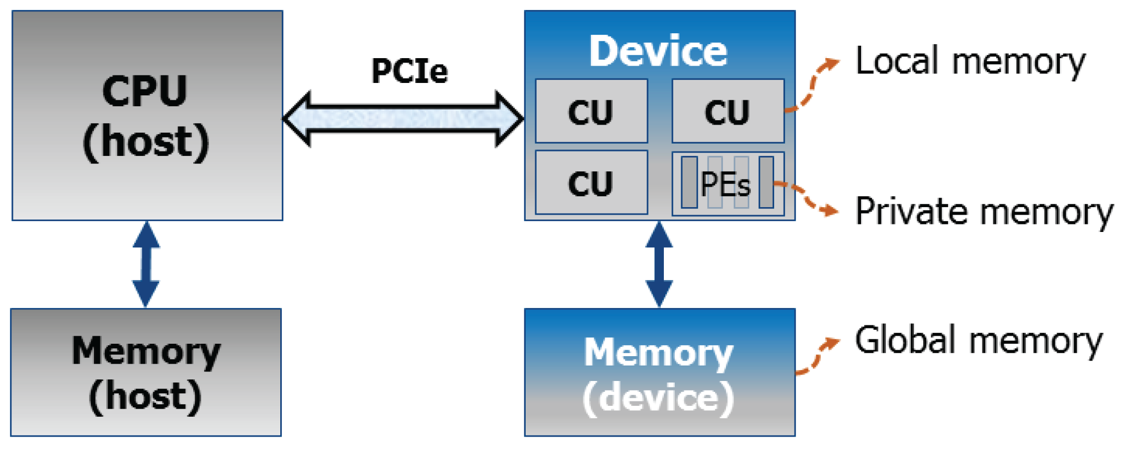
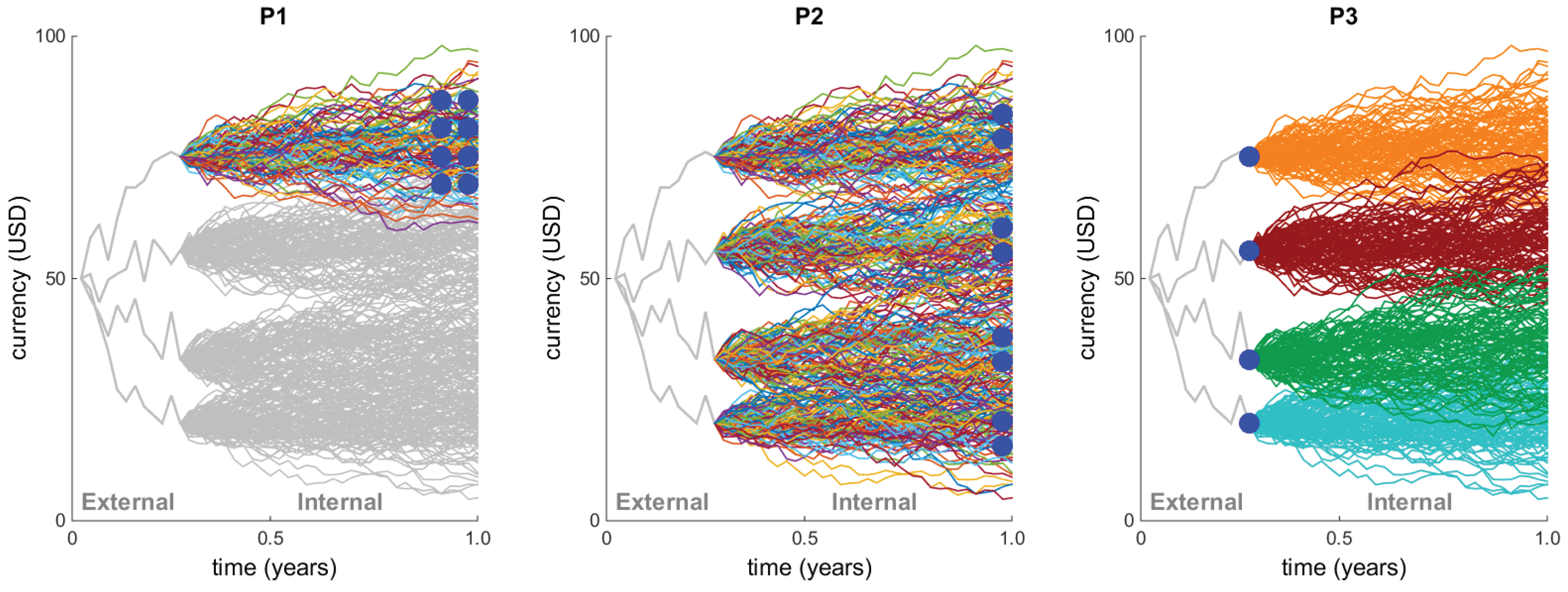
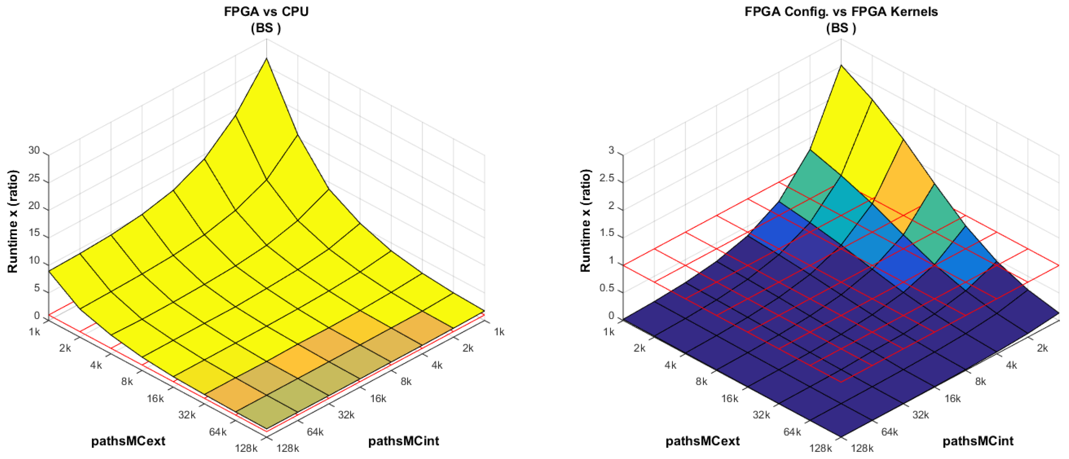
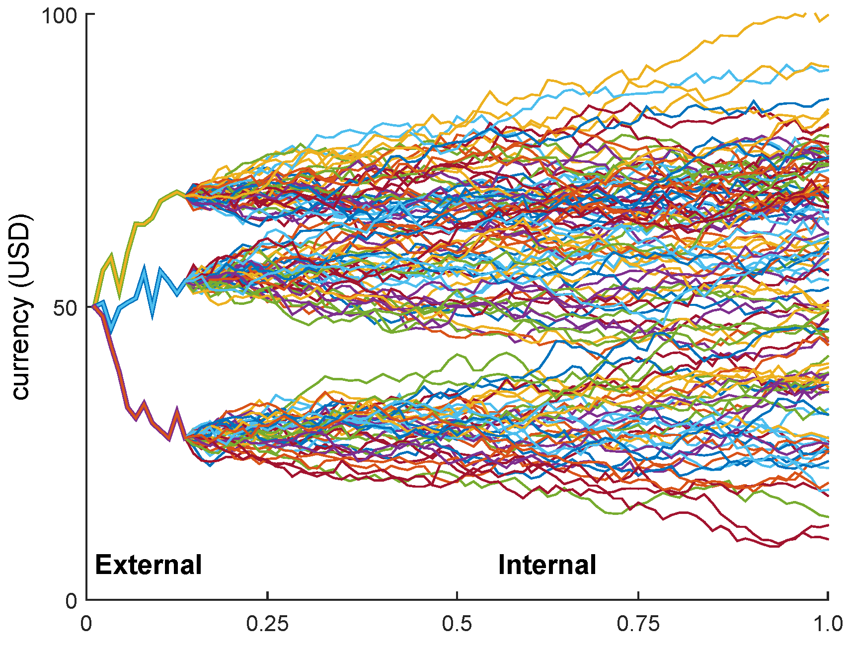
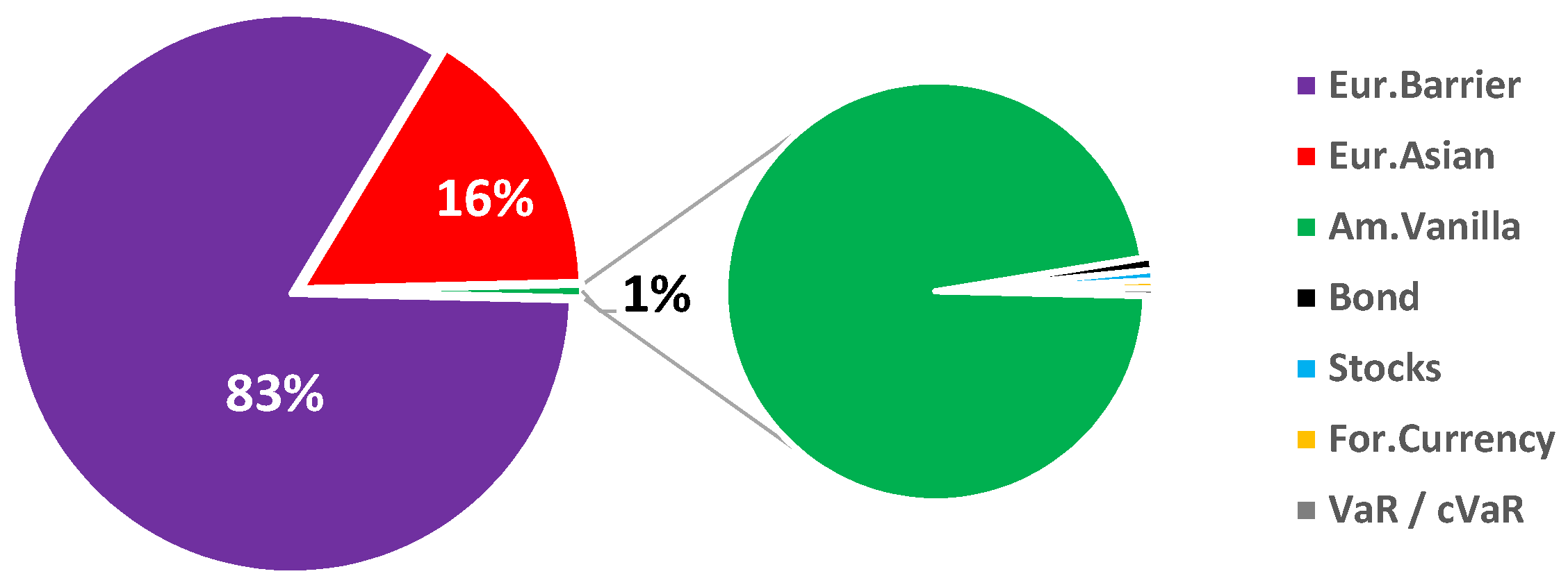
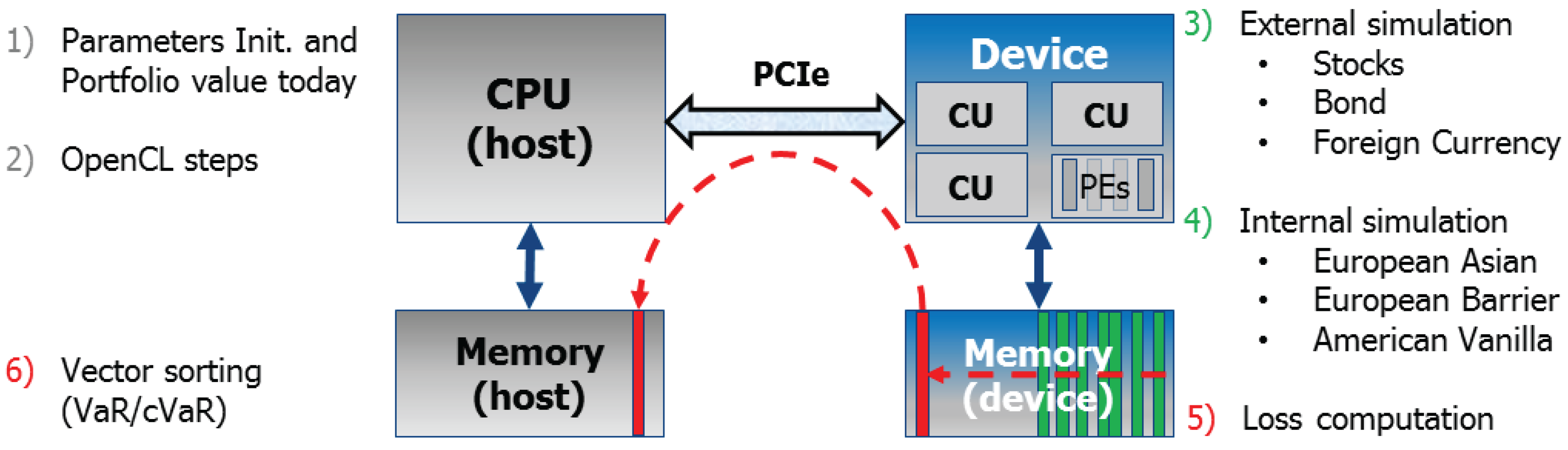
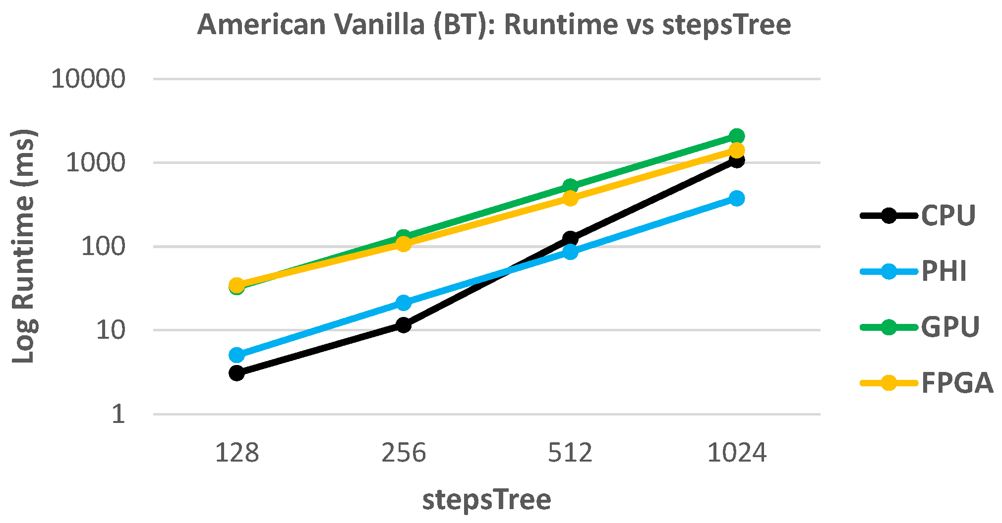
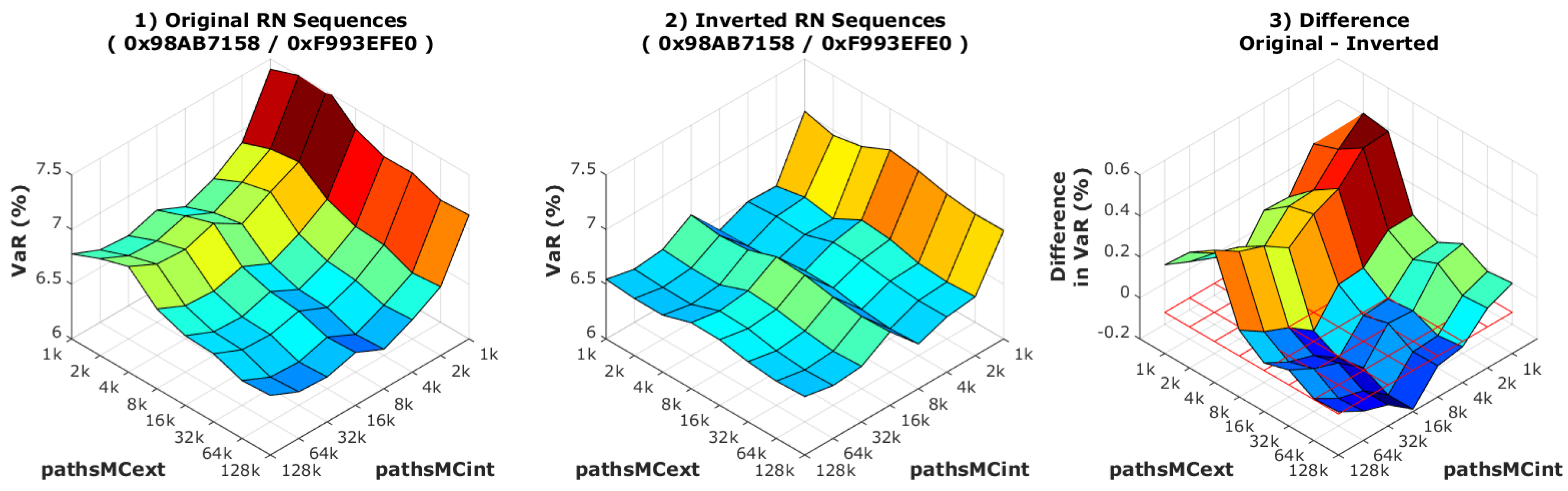
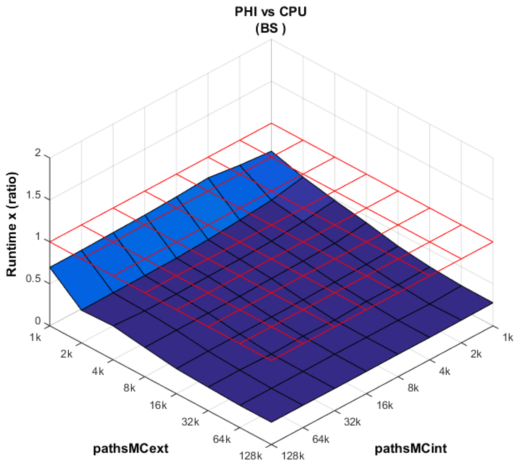
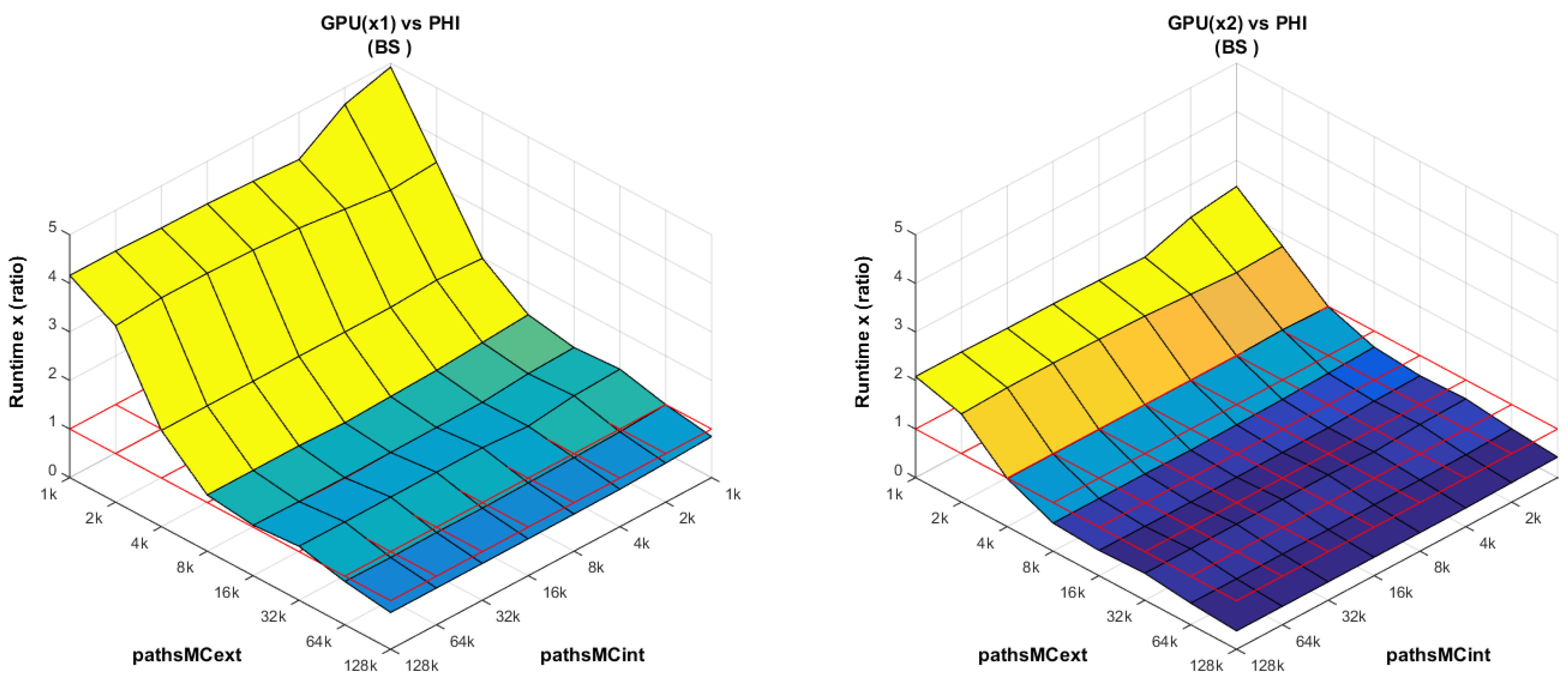
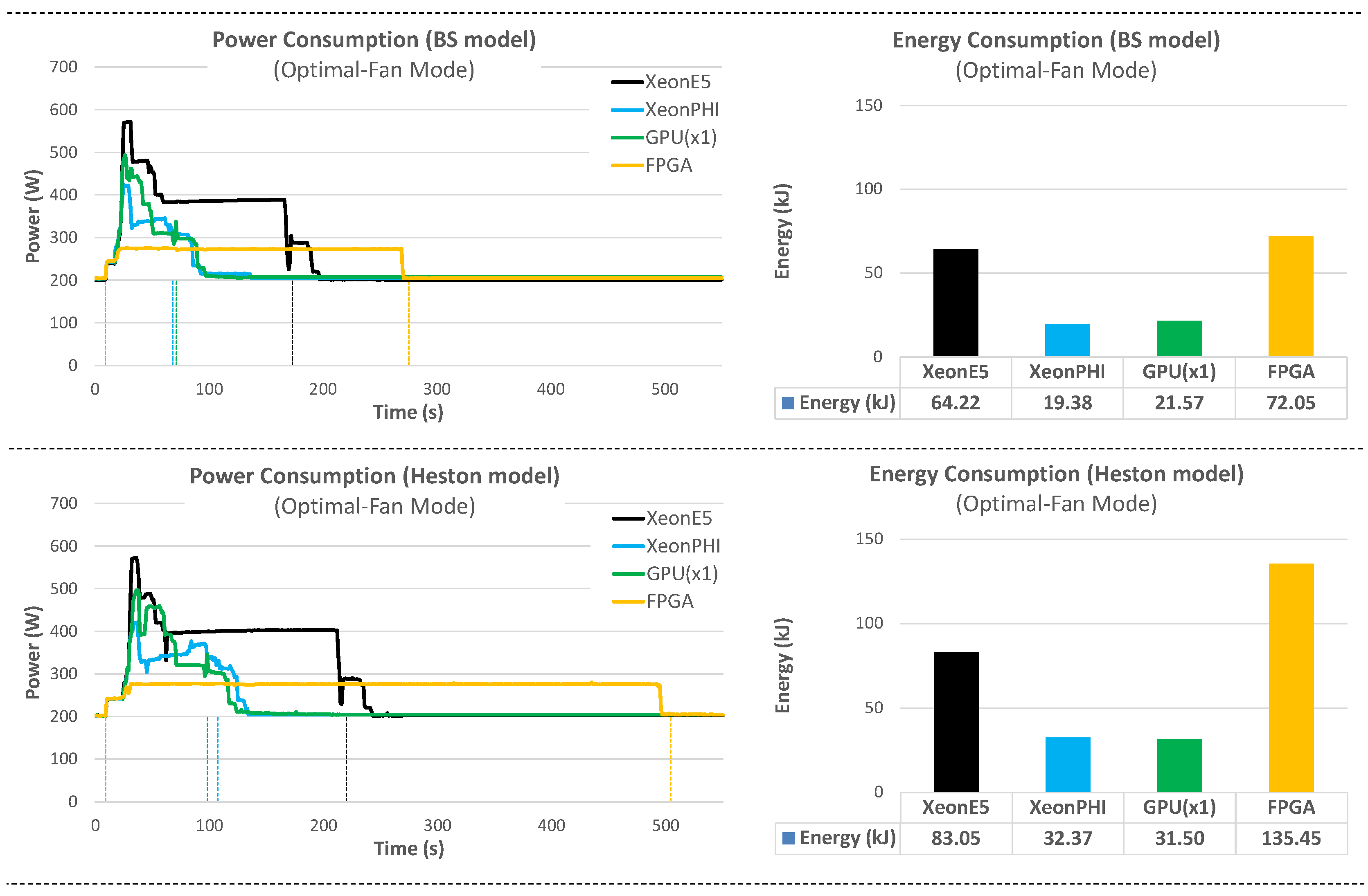
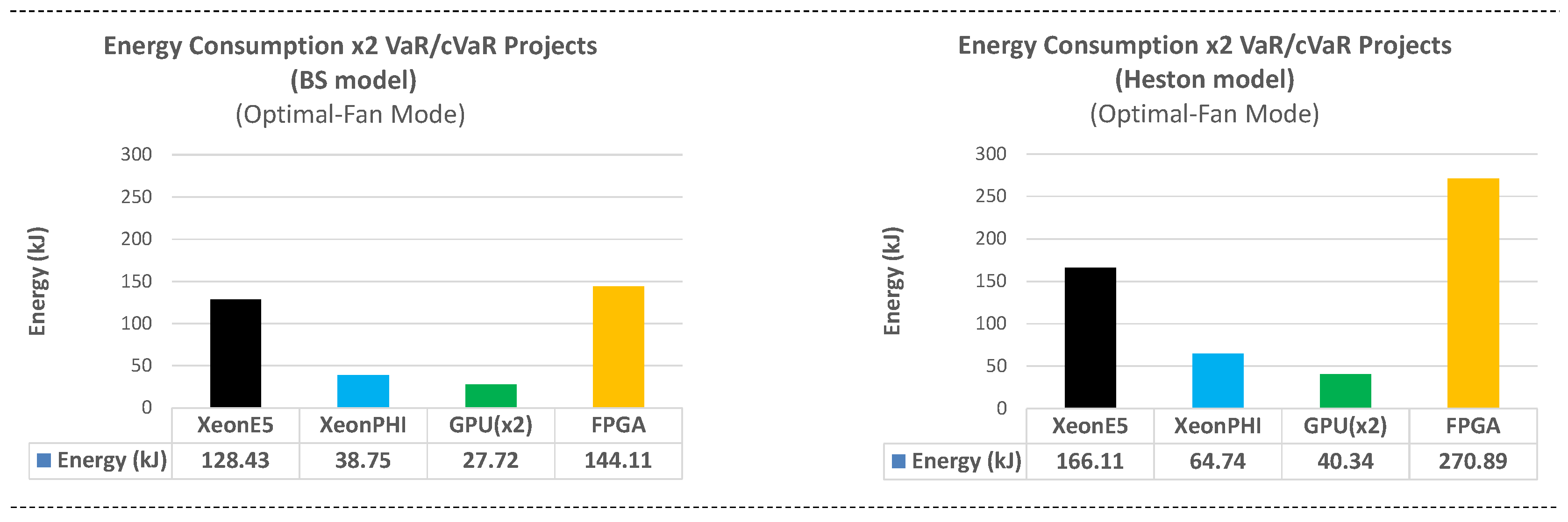