1. Introduction
In this paper, we study the valuation of index-linked cash flows under the assumption that index returns and the changes in nominal interest rates have significant dependence. The cash flows we consider are such that each payment is a product of two independent random variables: one is the index value, and the other may represent pure insurance risk or simply a constant. Typically, the index is a consumer price index or a wage index, but the index returns could also be interpreted as claims inflation, i.e., an increase in claims cost per sold insurance contract. Given a deep and liquid market of bonds linked to the same index as the cash flow, the natural market-consistent value of the cash flow is a best estimate of the non-index factor times the market-implied price of an index-linked zero-coupon bond. Here, we focus mainly on market-consistent valuation of index-linked cash flows when market-implied prices of index zero-coupon bonds are absent or unreliable.
A traditional approach to valuation of insurance cash flows is to assign a value corresponding to the discounted expected cash flow, where the discount factors match a yield curve bootstrapped from, e.g., current data on government bonds or interest rate swaps. However, if the cash flows depend on the development over time of an index that shows clear signs of dependence on changes in the yield curve, then the traditional valuation approach is inappropriate and possibly even a source of arbitrage opportunities. The importance of market-consistent valuation in life and pension insurance is well understood by insurance companies and regulators, and the theoretical foundation is well established and accessible in textbooks; see, e.g., [
1,
2,
3]. Moreover, the ideas of integrating traditional insurance valuation with financial no-arbitrage valuation can be found in the literature from the 1970s; see, e.g., [
4]. Many articles found in actuarial journals are based on the idea that it is possible to construct a portfolio of financial assets that replicates the unit in which a life insurance contract is expressed; see, e.g., [
5,
6,
7]. Valuation of unit-linked life insurance products with embedded options and guarantees is treated in, e.g., [
8,
9], and participating policies are analyzed in, e.g., [
10,
11,
12]. Valuation frameworks for pension liabilities and long-term health insurance are developed in [
13,
14], respectively. Market-consistent valuation in non-life insurance is a rather new subject treated in, e.g., [
15,
16].
The approach we promote for the valuation of index-linked cash flows requires accurate modeling of the dynamics of the yield curve of nominal interest rates. For this purpose, we choose a Heath–Jarrow–Morton (HJM) model in a discrete-time setting. HJM models, introduced in [
17], are flexible enough to realistically model the evolution of the forward-rate curve over time and are more appealing than short-rate models, since they directly model the evolution of the entire forward-rate curve. Key features of simultaneous changes in forward rates are easily investigated using, e.g., principal component analysis on historical yield-curve data. From a theoretical perspective, HJM models in continuous time are complicated models whose properties have posed challenges to probabilists. However, by now, they are among the standard interest-rate models (see, e.g., [
3,
18]), and generalizations of the models that allow for non-Gaussian driving noise processes are well understood; see [
19,
20].
We apply the valuation principles in [
3], in an HJM framework and based on historical yield-curve and index data, with the aim of setting up a credible valuation machinery for index-linked cash flows. The valuation formulas we derive allow us to understand how the volatility structure of the calibrated HJM model, the market-price-of-risk vector, the forecasts of trends in index values and interest rates and the necessary modeling assumptions affect the value of an index-linked cash flow. The index we consider in the empirical analysis is the Swedish Consumer Price Index (CPI), to which, for example, illness and accident insurance contracts often are linked. Market prices of CPI-linked bonds offer possibilities to investigate how the market’s anticipation of future price inflation can be understood in terms of our valuation machinery.
The suitable time grid (weekly, monthly or quarterly, say) for the HJM modeling of the dynamics of the yield curve might be finer than the time grid for the updates of index values. Even if frequently-updated index values are available, seasonal effects and problems with data quality might suggest that a coarser time grid for the index values is preferable. Moreover, many insurance liability cash flows depend on yearly updated values of a consumer price index, whereas historical data of yearly yield curve changes are not sufficient for efficiently parameterizing an HJM model. We investigate the effects of different time scales on the valuation of the index-linked cash flows.
In [
21], a three-factor HJM model is used to model the joint dynamics of a U.S. consumer price index and the real and nominal U.S. Treasury yield curves, with the aim of pricing and hedging both inflation bonds and conventional nominal bonds. The basic idea is to exploit the analogy between nominal and real interest rates and a consumer price index, on the one hand, and two currencies and an exchange rate, on the other hand. The foreign-exchange analogy has appeared earlier also in [
22]. The paper [
21] discusses both model selection and validation issues and uses the model to price options written on the consumer price index. In [
23], the question of how and under what conditions an inflation-index bond can be replicated by dynamically trading in nominal bonds is investigated.
Our main contributions in this paper can be summarized as follows. Firstly, we present an approach for transparently assigning a monetary value to a stochastic cash flow that does not require full knowledge of the joint dynamics of the cash flow and the term structure of interest rates. Secondly, we investigate in detail model selection, estimation and validation in a Heath–Jarrow–Morton framework. Finally, we analyze the effects of model uncertainty on the valuation of the cash flows and how forecasts of cash flows and interest rates translate into model parameters and affect the valuation.
The outline for the paper is as follows. In
Section 2, we introduce principles for market-consistent valuation of cash flow that will form the basis for our valuation machinery and give a summary of the discrete-time HJM framework.
Section 3 derives valuation formulas for index-linked cash flows taking the modeling at different time scales into account. The proofs containing rather lengthy computations are placed at the end of the paper in
Appendix.
Section 4 presents model selection and model validation issues, describes the data and presents the empirical findings and statistical analysis.
Section 5 applies the valuation machinery and presents and interprets the numerical results. Finally, the discussion in
Section 6 concludes the paper.
2. Preliminaries
We work in a discrete-time setting with time points , where denotes the current time. We consider a filtered probability space , where with denoting the information available at time t. The probability measure , called the real-world probability measure, is assumed to describe future observations of cash flows and price processes. Typically, it is chosen so that relevant features of historical data are plausible for future values of cash flows and price processes. The expectation operator with respect to is denoted by . In expressions involving matrix multiplications, vectors are taken to be column vectors. We use the notation for the scalar product and for the Euclidean norm.
We consider a given currency that applies to all price processes and cash flows. A cash flow here is a random vector , where is the amount due at time t. The price at time t of the cash flow X is denoted by .
For market-consistent valuation of insurance cash flows, a useful approach is presented in [
3]. Here, we give a brief outline of the approach. We set up models and validation procedures in subsequent sections.
We assume that all cash flows
are
-adapted with integrable components and write
. A state price deflator
is a strictly positive random vector with normalization
. We interpret
as a stochastic discount factor transporting cash amounts
at time
t to values at time 0. The set of cash flows that can be valued relative a given state price deflator
ϕ is given by:
and the price process
for a cash flow
is defined by:
A price process
is called consistent with respect to a state price deflator
ϕ if the deflated price process
is a
-martingale. Using the tower property of conditional expectation, we see that the definition in Equation (
1) implies that deflated price processes are
-martingales,
Let
denote the price at time
t of a non-defaultable zero-coupon bond (ZCB) with maturity
. By convention,
. The one-period risk-free rollover
and the value of one unit of the corresponding bank account at time
t are defined by
for
,
for
, and
. From the definition Equation (
1) and the fact that
is
-measurable, it follows that the process
is a strictly positive
-martingale with an expected value of one (Lemma 2.17 in [
3]). Therefore, we may define the probability measure
, equivalent to
, by
for any
-measurable event
A for
. In particular,
is the Radon–Nikodym derivative for
with respect to
on
. The probability measure
, called the risk-neutral probability measure, is the equivalent martingale measure for the bank account numeraire
:
is a
-martingale (Lemma 11.5 in [
3]). We write
for the expectation operator with respect to
.
By a standard change of the numeraire argument (Lemma 11.4 in [
3]),
Therefore, using the linearity of conditional expectations, the price at time
t of the cash flow
can be expressed as:
i.e., the risk-neutral value at time
t of the cash flow
. Unless we are considering a very simple cash flow, the joint distribution under
of the
and
is hard to determine, and the effect on the valuation of dependencies between interest rates and cash flows is hard to assess. Therefore, although valuation using state price deflators is equivalent to risk-neutral valuation, the former is more natural for cash flows with distributions that cannot be easily assessed from market prices of financial contracts.
From a modeling perspective, we may first decide on a model for the (forward) interest-rate dynamics under , such that the model may, given a convenient change of measure from to , yield dynamics under that are in line with historical observations of interest rates. The measure transformation is typically determined by the market-price-of-risk function, which should be chosen so that the model parameters under can be estimated and the model validated on historical data. The interest-rate model under and the market-price-of-risk function determines the model for the state price deflators under , which can be extended into a joint model under of both cash flows and state price deflators. This approach to setting up the valuation framework and validating the models of historical data is presented below.
The Heath–Jarrow–Morton Framework
The forward rate at time
t for maturity
u is defined by:
and the price of a ZCB can be expressed in terms of forward rates as:
We assume an HJM framework with the forward rate dynamics:
where the innovation vector
is
-measurable. The risk-neutral measure
is chosen so that
is independent of
under
. The consistency condition for an arbitrage-free pricing system is:
where
is the value of the bank account at time
t. The consistency condition can be written (see ([
3], pp. 98–99) for details):
where the function
h is defined by:
with
. If the expectation in Equation (
3) is finite, we get
for
, and
. We choose
, so that the components of
are independent standard normal random variables under
. Then,
and:
Now, let
, where
is called the market price of risk at time
t. We require that
is
-measurable. The forward rate dynamics can be expressed as:
where:
The density process
is chosen as:
Notice that, given sufficient integrability (Novikov’s condition),
is a
-martingale and
is a
-martingale. This choice of density process implies that the
are independent and standard normally-distributed under
. Indeed, the fact that for an
-measurable
X it holds that:
implies that:
which further implies that:
We observe that the moment generating function of the random vector of length is the moment generating function of the -dimensional standard normal distribution. The claim follows.
3. Valuation of an Index-Linked Cash Flow
We consider the valuation of a cash flow formed by two independent components: a pure insurance risk component and an index component. More specifically, we consider the value of the cash flow
at time
, where
and
are
-measurable and independent under
. The meaning of
k and
T will be made clear below. According to Equation (
1), the value today of the cash flow
is
, where
. If
denotes the value at time
of an inflation index and if there is a deep and liquid market of (coupon-bearing) inflation-linked bonds, then the market prices determine the market price
of the cash flow
I, which is the cash flow of a real zero-coupon bond maturing at time
.
We focus on the case when index values and nominal interest rates are dependent and when is not trivially determined by the market prices of index-linked bonds. In this case, modeling of the joint dynamics of the index and nominal interest rates is required. Whereas data are available that enable the selection of a plausible model for the dynamics of interest rates, the index value data may be limited in size and quality. Therefore, we want a transparent approach to cash-flow valuation where the value factors into a product, where one factor is the expected value of the part of the index value that cannot be explained by interest rates, and the other factor, completely specifying a generally accepted HJM forward-rate model, is the monetary value of the part of the index value that is explained by the interest rates. We want the first factor to allow for subjective input, such as an assumption of a particular long-term trend in the index value. Subjective views may be attractive for stress testing, or internal valuation purposes, or imposed exogenously by a supervisory authority.
For the discrete-time forward-rate dynamics, the time unit is commonly chosen large enough to avoid unnecessary noisy forward rate data, but small enough for the model to capture relevant time series features. However, for valuation purposes, it may be of interest to consider the forward-rate dynamics on a coarser time grid, e.g., with yearly observations instead of quarterly observations. Let be an integer and consider a new time unit corresponding to k original time units. We use the superscript k to denote that time is measured in units of k original time units. Let be the log return of some index between time and time : . Without loss of generality, we set . If the original time unit is a fraction of a year, then the series may not be available or can be hard to model accurately due to seasonal effects and, in the case of a price index, so-called price stickiness; prices are not rapidly updated as costs and demands change in the economy. Therefore, it may be more attractive to consider changes in the index over longer time periods (one year, say).
Given the independence between the pure insurance risk variable
and
,
. Hence, if we determine a random variable
Z, such that
and
are independent, then
, where:
Notice that the market price of risk does not affect the value . In order for this approach to computing to have practical utility, we want Z to be an affine function of forward rates for , so that Equation (7) is easily computed using the HJM dynamics under . Moreover, we want Z to be a rather simple expression in terms of some forward rates, so that the distribution of is easily assessed from historical data or economic arguments. If the market price of risk is an affine function of forward rates and if the and the are jointly normally-distributed, then the independence of and is equivalent to , which is more easily testable. Notice that Z could be taken as the orthogonal projection of onto the linear space spanned by . However, the restriction of Z to an affine function of forward rates appears more useful.
Based on empirical investigations presented in
Section 4, in the case when the index is chosen as a consumer price index, here, we choose
Z so that the right-hand side of Equation (
6) is expressed as:
Recall that is the index log return from time to time and that is the continuously-compounded spot rate at time of a ZCB maturing at time . Both and are observable at time .
The traditional value at time 0 assigned to an insurance cash flow
at time
is
,
i.e., the discounted best estimate. In Proposition 1 below, we compute the market-consistent value
and compare it to the traditional value of the cash flow. The proof of the proposition is found in
Appendix.
Proposition 1. Suppose that:
are uncorrelated under .
Then:
If, further, the market price of risk λ
is a constant vector, then:
The quantities and are given by:
and, for ,
and, for ,
where is the smallest integer larger or equal to the nonnegative number x.
Notice that under the assumption of Proposition 1 and a constant market-price-of-risk vector λ, the valuation ratio:
is an expression in terms of σ, λ,
k and
T. In particular, it does not depend on the current term structure of forward rates. Moreover the dependence on the market price of risk λ is rather easily analyzed by writing:
In
Section 4, we present an approach to estimating the function σ from historical forward-rate data. We also consider the modeling of the market price of risk vector
as an affine function of past forward rates and present a testing procedure for determining whether
may be taken as a constant vector λ. Finally, in
Section 5, we investigate numerically, based on historical data, the market-consistent valuation of an inflation-linked insurance cash flow and analyze how the market-consistent value differs from the value based on traditional valuation.
4. Model Selection and Validation
The Swedish Riksbank provides market prices of Swedish government bills with maturities of 1, 3, 6 and 12 months and government bonds with maturities of 2, 5, 7 and 10 years from 1992 to 2014. We choose the time unit as a quarter of a year, and here, we let
denote the time of the oldest market prices of the historical sample. Historical zero-coupon yield curves:
where
is the continuously-compounded spot rate at time
t for maturity
u, are obtained by a standard bootstrap procedure assuming linearity in
R between observed market rates. Moreover, we assume that
for
,
i.e., the rate for a maturity further away than 10 years is set equal to the 10-year rate.
Notice that
and that the forward rates at time
t are given by
and:
We assume an HJM framework with a volatility function satisfying
. This simplifying parametrization is rather common; see, e.g., Example 6.6 in [
18,
21,
24] and Section 5.4 in [
25]. Discussions of possible shortcomings and remedies of such a parametrization for HJM models designed for interest-rate derivative pricing can be found in, e.g., [
26,
27]. We assume that the market price of risk is a function of the previous forward rates and get the forward rate dynamics:
where
and
. Recall that the conditional distribution of
given
is a multivariate standard normal distribution under the real-world measure
. We define forward rate changes by:
We would like to estimate the functions λ and σ simultaneously on historical data for sufficiently flexible parameterizations of the two functions, for instance by maximum likelihood estimation. Unfortunately, this approach will not work well. Instead, we perform a two-stage estimation by, in the first stage, considering λ to be a constant vector and estimating σ, and, then, in the second stage, considering the estimate of σ to be the true, but unknown volatility function and estimating a parametric model for λ by maximum likelihood estimation. Finally, we validate our selected parametric model.
4.1. The Volatility Structure of Changes in the Forward Rates
As the basis for a statistical analysis of historical forward rate dynamics, we choose the vectors:
where
and
, since the elements in these vectors roughly correspond to the changes in spot rates observable in the market data. According to our modeling assumption,
, where:
and Σ is an
-matrix with
as the
j-th row. If the covariance matrix of
is small and does not vary much over time, then the covariance matrix of
is approximately
. In particular, then, the function σ, the volatility structure, can be estimated from the sample covariance matrix of historical forward rate changes. To this end, we conduct a principal component analysis of the sample covariance matrix of vectors of forward-rate changes for the chosen set of maturities.
We denote eigenvalue
i by
and eigenvector
i by
,
. From the eigenvalues shown in
Table 1, we get that
, which means that 89% of the variance is explained by the first two components.
Table 1.
Eigenvalues () of the sample covariance matrix of forward rate changes ().
Table 1.
Eigenvalues () of the sample covariance matrix of forward rate changes ().
| | |
| | |
| | |
| | |
| | |
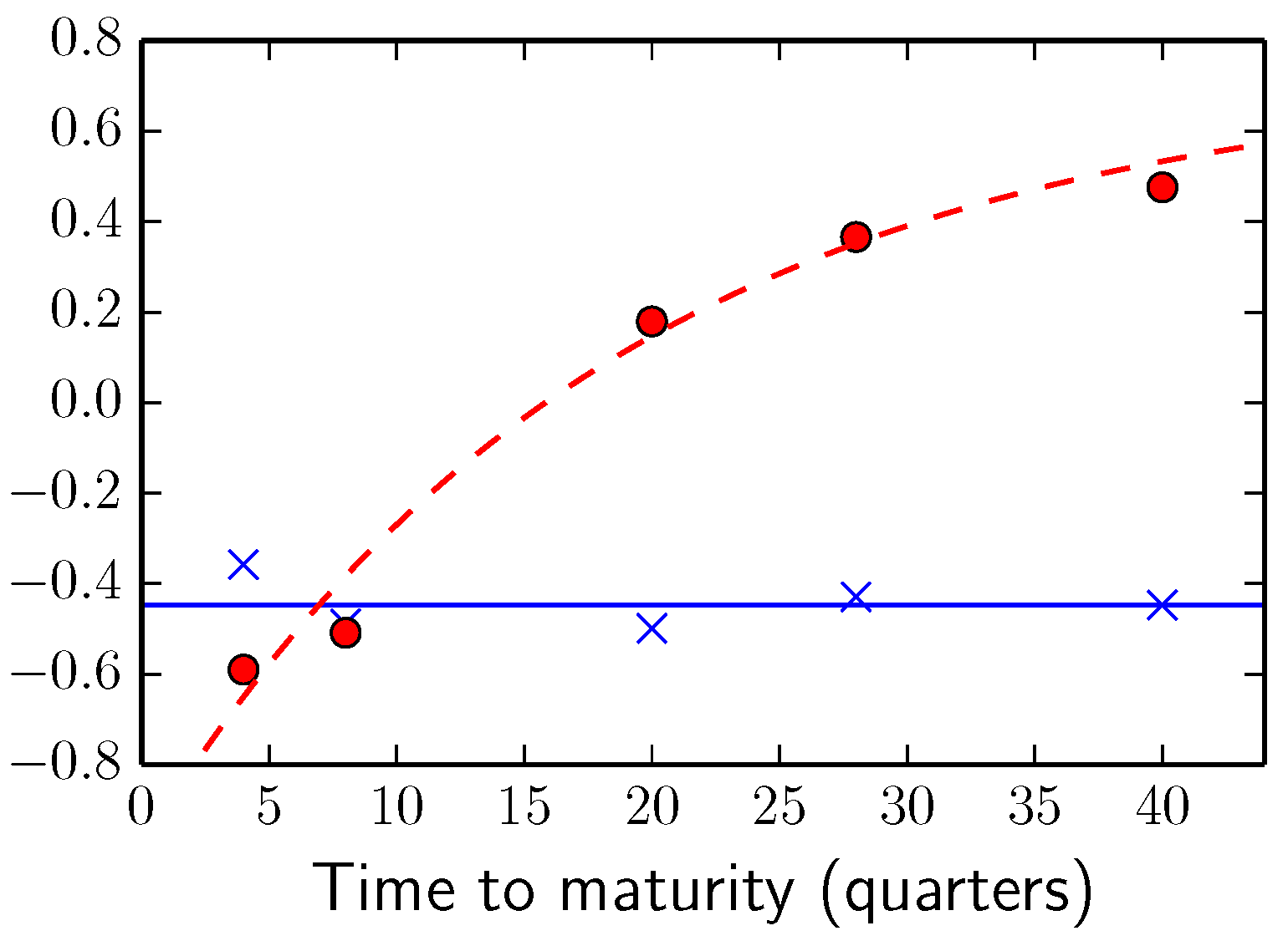
In order to have a smooth dependence on maturity, we fit functions
and
to the eigenvectors
and
, respectively. Plots of the eigenvectors suggest functions of the following form:
and
. Other parameterizations are possible; see, e.g., Example 6.6. in [
18].
The vectors:
should satisfy
,
and
. To satisfy the first condition, we set
. Since
is independent of
m, the third condition can be written
, which implies that
, and we get:
We let
denote the
i-th component of the second eigenvector
and find the pair of arguments
that minimizes:
We are almost done, but
, so a slight modification is needed to get
and
orthonormal. Setting:
yields the desired result. To summarize,
,
, and:
The eigenvectors
and
are plotted together with the functions
and
in
Figure 1.
Figure 1.
Eigenvectors (blue crosses) and (red circles) together with the functions (blue solid line) and (red dashed line).
Figure 1.
Eigenvectors (blue crosses) and (red circles) together with the functions (blue solid line) and (red dashed line).
To compensate for only considering variance in the plane spanned by
and
, due to the reduction in the dimension of the driving input noise from five to two, we must have higher variances along these vectors in our model than what we see in the data. To this end, we find the κ that minimizes:
We get and set , with for , where .
4.2. The Market Price of Risk and Model Validation
We now assume the forward rate dynamics given by
, where Σ is known, set to the estimate above, and
is an i.i.d. sequence of standard normal bivariate vectors under
. Since:
and
and
are orthonormal,
Hence, the forward-rate dynamics
can be rewritten as:
The left-hand side in Equation (
9) corresponds to a known affine transformation of observed changes in forward rates for the chosen maturities. We assume that the market price of risk is an affine transformation of previous forward rates and, therefore, express Equation (
9) as:
where
,
and
and the
are unknown vectors. Notice that the conditional distribution of
given
is a bivariate normal distribution with uncorrelated components with unit variances and mean vector
. Therefore, maximum likelihood estimation of
and the
coincides with ordinary least squares estimation:
with:
and:
Maximum likelihood values for different numbers of non-zero
are shown in
Table 2. Likelihood-ratio tests based on these values suggest that we should not use more than three non-zero
.
Table 2.
Maximum log-likelihood values.
Table 2.
Maximum log-likelihood values.
| Number of Non-Zero | Non-Zero | Maximum Log-Likelihood |
|---|
| 6 | , , , , , | |
| 5 | , , , , | |
| 4 | , , , | |
| 3 | , , | |
| 2 | , | |
| 1 | | |
| 0 | - | |
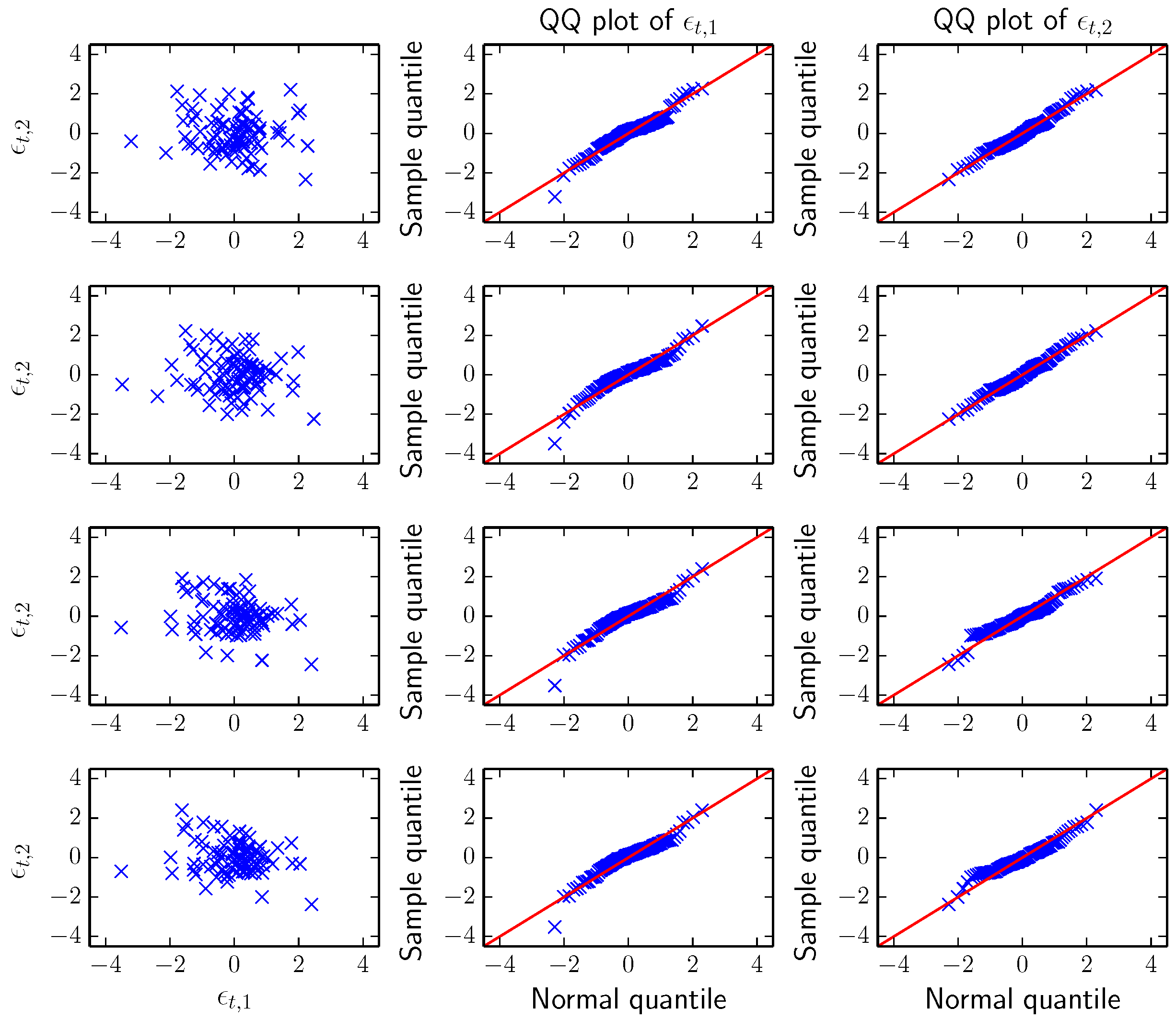
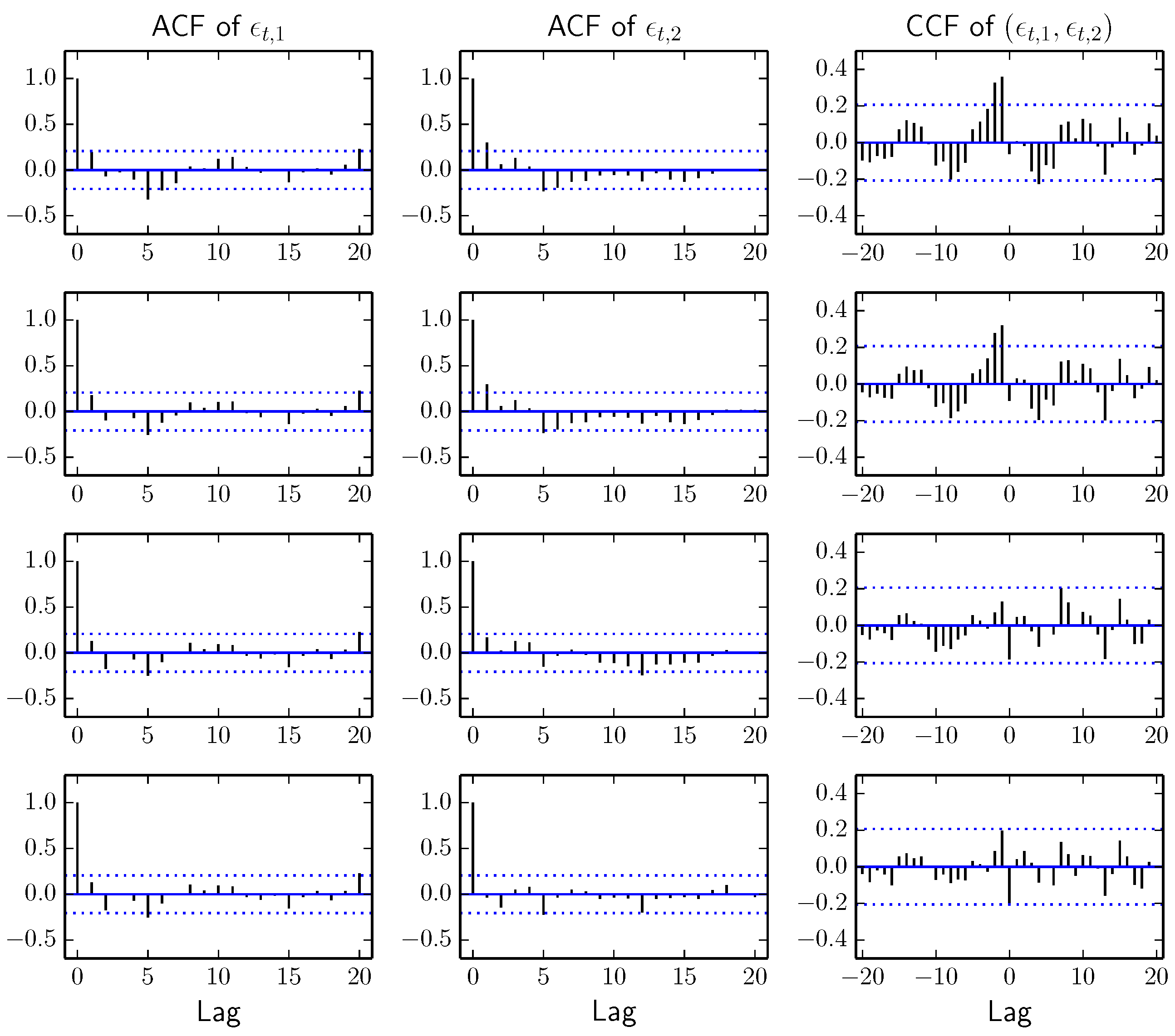
Scatter and QQ plots of the innovations for the cases with 0, 1, 2 and 3 non-zero
, respectively, are shown in
Figure 2, and auto- and cross-correlations are shown in
Figure 3. Since the innovations look very similar in all four cases, we select the simplest model,
i.e., the model with a constant market price of risk.
Figure 2.
Scatter and QQ plots of the innovations for the cases with 0, 1, 2 and 3 non-zero , respectively.
Figure 2.
Scatter and QQ plots of the innovations for the cases with 0, 1, 2 and 3 non-zero , respectively.
Figure 3.
Auto- and cross-correlations of the innovations for the cases with 0, 1, 2 and 3 non-zero , respectively.
Figure 3.
Auto- and cross-correlations of the innovations for the cases with 0, 1, 2 and 3 non-zero , respectively.
Writing
and using the invariance property of the maximum likelihood estimator, the maximum likelihood estimator of λ is given by:
We get
. Notice that
, so we may calculate confidence regions for λ using:
where
g is a bivariate standard normal random variable. We have:
where
is chi-square distributed with two degrees of freedom. We get
by solving
.
4.3. The Relation between the Consumer Price Index and the Short Rate
Statistics Sweden (
Statistiska centralbyrån in Swedish) provides monthly values of the Swedish Consumer Price Index (CPI). However, we prefer to study changes over a one-year horizon to get rid of seasonal effects and to get less sensitivity to price-stickiness. We denote the change in the consumer price index for year
t by
,
i.e.,
, and the risk-free rollover for the same year by
. Notice that
is known already at time
, while
is not known until time
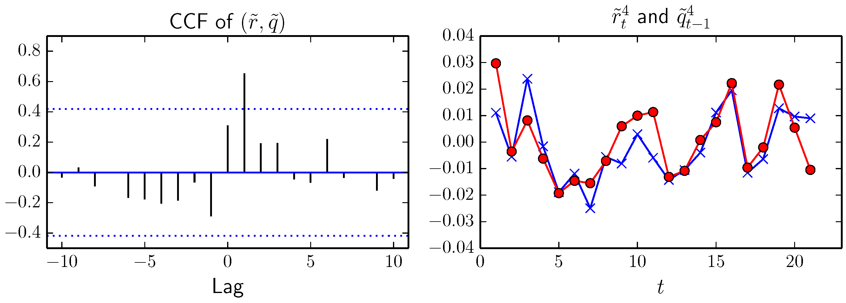
. Moreover, if we remove linear trends from
q and
r and denote the detrended values by
and
, respectively, we get the strongest cross-correlation when
lags
by one year (see
Figure 4). Thus, it is natural to study the differences
.
Figure 4.
Cross-correlations between and and time series plots of (blue crosses) and (red circles).
Figure 4.
Cross-correlations between and and time series plots of (blue crosses) and (red circles).
We define:
and notice that the factorization condition in Proposition 1 is satisfied if the
and
are jointly normally distributed and
.
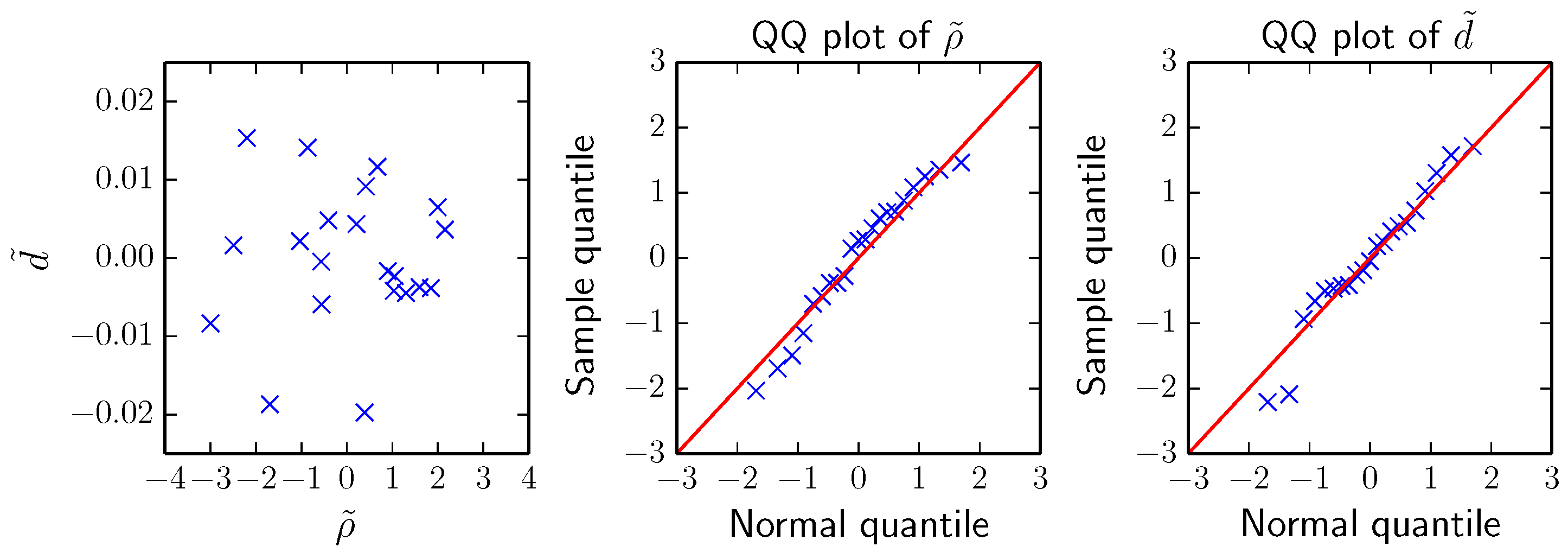
The
are calculated using the estimated constant market price of risk and the observed innovations. We remove linear trends from
d and ρ and denote the detrended values by
and
, respectively. The sample standard deviation of
is
. Scatter and QQ plots of
and
are shown in
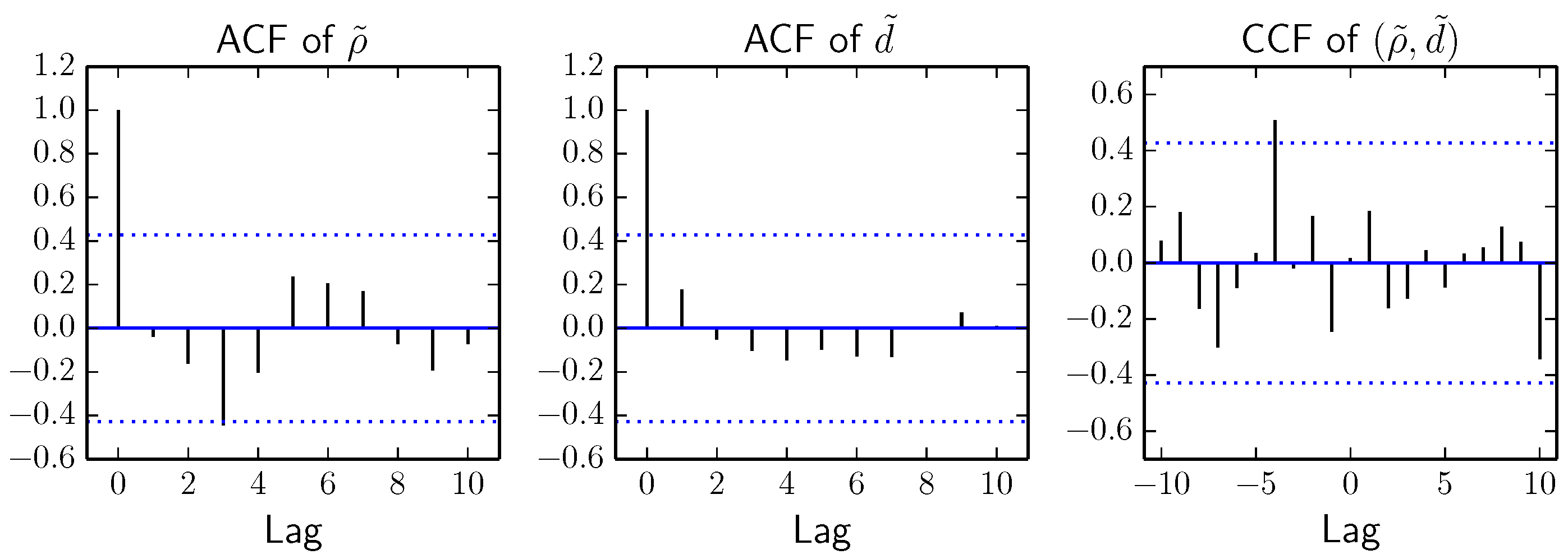
Figure 5, and auto- and cross-correlations are shown in
Figure 6. These plots suggest that
and
are uncorrelated and jointly normally distributed, hence independent.
Figure 5.
Scatter and QQ plots of and .
Figure 5.
Scatter and QQ plots of and .
Figure 6.
Auto- and cross-correlations of of and .
Figure 6.
Auto- and cross-correlations of of and .
5. Model-Based Valuation
In this section, we value a cash flow linked to the Swedish CPI using our model. We consider the cash flow
, where:
with
.
According to Equation (
1), the value of
X today is
. However, in practice, one often assumes independence between the interest rates used for discounting and the claims payments, and under this assumption, today’s value is
.
We set
and let
be the change in CPI for year
t. The analysis in
Section 4 suggests that the
are normally distributed and that the factorization condition in Proposition 1 is satisfied. It also suggests that a constant market price of risk is a reasonable assumption. Assuming that
represents some actuarial risk independent of price inflation and interest rates, we get:
and:
where
, from Proposition 1. We assume that:
where the parameters are set to the estimates from
Section 4.
The value
is independent of the market price of risk λ, but depends on the trend in future price inflation (relative interest rates). We assume that
is normally distributed with mean
for some constant trend
c and standard deviation
, and we get:
Values of
for different trends are shown in
Table 3.
Table 3.
Values of with .
Table 3.
Values of with .
| T | | | | | |
|---|
| 1 | 0.961 | 0.980 | 1.000 | 1.020 | 1.041 |
| 2 | 0.923 | 0.961 | 1.000 | 1.041 | 1.083 |
| 5 | 0.819 | 0.905 | 1.000 | 1.105 | 1.221 |
| 10 | 0.670 | 0.819 | 1.000 | 1.221 | 1.492 |
At this point, it should be mentioned that if there exists a deep and liquid market of bonds linked to the same index as the insurance liability cash flow, then a market-consistent value of the cash flow is given by , where denotes the price of an index-linked zero-coupon bond maturing at time t. In our case, is the price paid today for receiving the amount at time t.
Swedish CPI-linked bonds (often called real bonds) are either bought at auctions held by the Swedish National Debt Office (
Riksgälden in Swedish) or over-the-counter (OTC) in the secondary market. All OTC trades are reported to Nasdaq OMX, so there is some market data available. Market rates on 28 November 2014 (the last day of our observation period) are shown in
Table 4. These rates should be interpreted as the yields to maturity given that the CPI remains at today’s level until the maturity date.
Table 4.
Market rates (in percent) of Swedish Consumer Price Index (CPI)-linked government bonds on 28 November 2014.
Table 4.
Market rates (in percent) of Swedish Consumer Price Index (CPI)-linked government bonds on 28 November 2014.
| Name | Years to Maturity | Average Rate |
|---|
| RGKB 3105 | | |
| RGKB 3107 | | |
| RGKB 3102 | | |
| RGKB 3108 | | |
| RGKB 3109 | | |
| RGKB 3104 | | |
Now, say that we are interested in the price of a real ZCB maturing in 10 years. The average rate of the bond maturing in 10.5 years (RGKB 3109) suggests a rather different 10-year rate than what a linear interpolation of the average rates of the bonds maturing in 7.5 and 14.0 years (RGKB 3108 and RGKB 3104), respectively, do. However, it seems reasonable to conclude that the 10-year real zero rate lies somewhere between
and
, which implies that
. Using the nominal forward rates bootstrapped in November 2014, we get
. Thus,
which corresponds to
.
From
Section 3, we get the valuation ratio:
where:
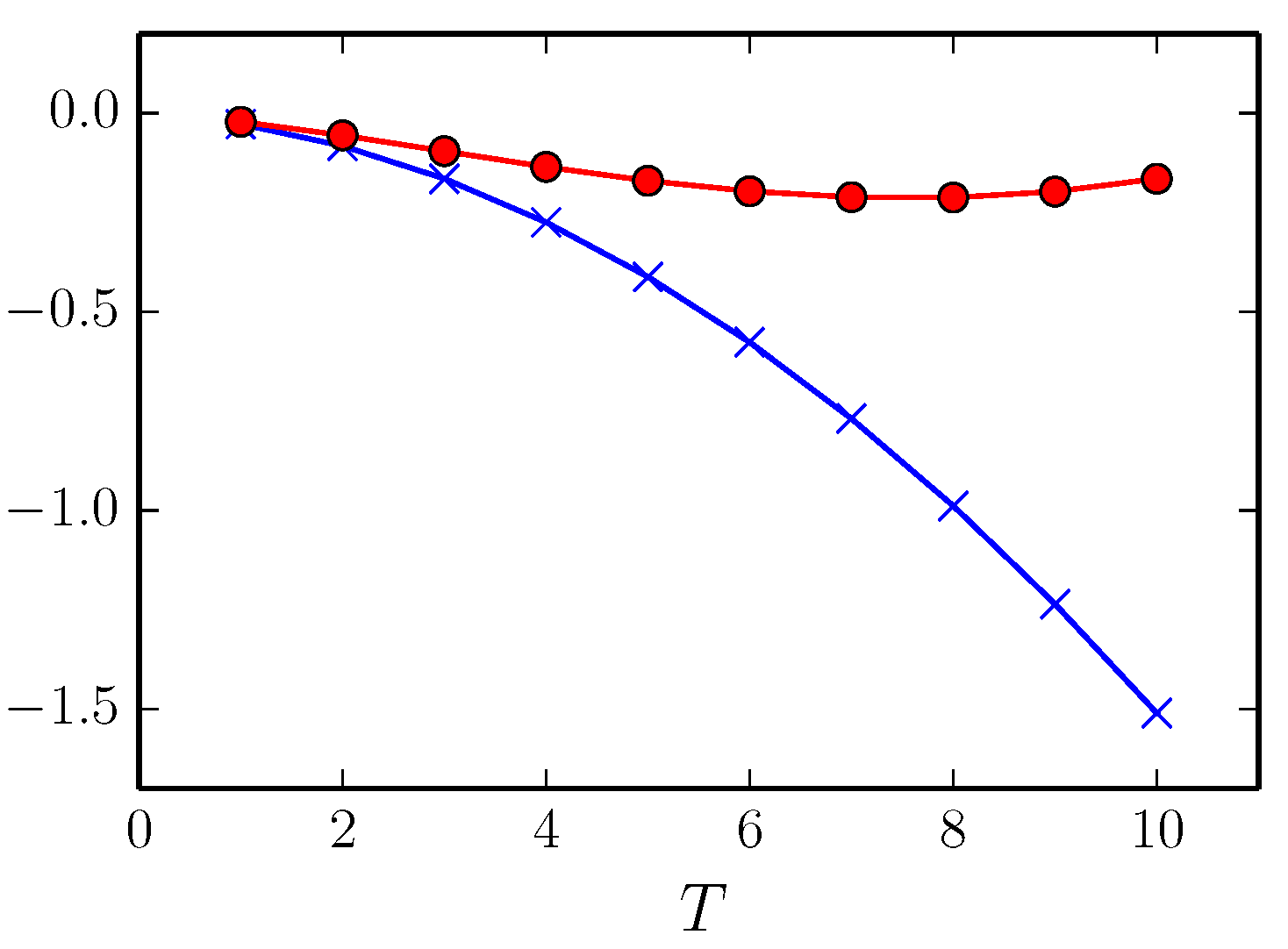
The valuation ratio depends on the market price of risk λ, but is independent of the trend in future inflation. Plots of
and
are shown in
Figure 7.
Figure 7.
Plots of (blue crosses) and (red circles), respectively.
Figure 7.
Plots of (blue crosses) and (red circles), respectively.
From Equation (
10), we get that
is normally distributed with mean
and variance
. Thus,
is log-normally distributed with mean:
Point estimates and confidence intervals of
for different values of
T are shown in
Table 5.
Table 5.
Mean and confidence interval of and valuation ratios for the market prices of risks 0 and .
Table 5.
Mean and confidence interval of and valuation ratios for the market prices of risks 0 and .
| T | | | 95% CI of | |
|---|
| 1 | 1.000 | 1.011 | (1.004, 1.019) | 0.994 |
| 2 | 0.999 | 1.028 | (1.007, 1.049) | 0.983 |
| 5 | 0.991 | 1.059 | (0.965, 1.160) | 0.925 |
| 10 | 0.935 | 0.884 | (0.638, 1.194) | 0.780 |
A market price of a risk vector defines expected future forward rate curves via the expression:
The expected forward rate curve in five years (
) given the market price of risk
is plotted as a black thick solid line in
Figure 8.
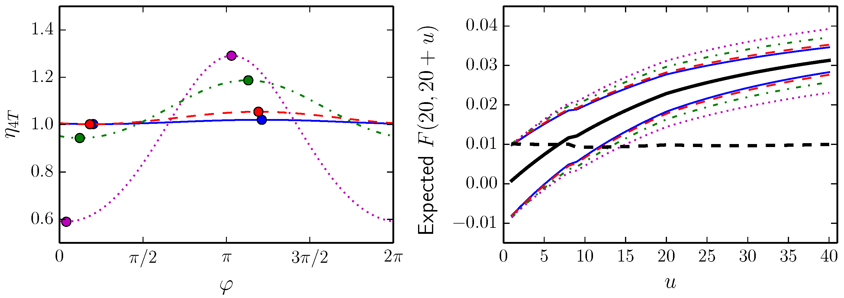
Figure 8.
Valuation ratios (left) and forward rate curves in five years for the minimum and maximum valuation ratios (right). The blue solid line, the red dashed line, the green dot-dashed line and the magenta dotted line correspond to , respectively. The black thick solid and dashed lines represent the market prices of risk and , respectively.
Now, consider market prices of risk of the type:
where
here denotes the estimate and
. Given
T and under the assumption that historical observations are representative for future conditions, these market prices of risk correspond to equal-probability valuation ratios and expected forward-rate curves. The valuation ratios and expected forward-rate curves in five years corresponding to the maximum and minimum valuation ratio, respectively, are plotted in
Figure 8.
Any belief in a future yield curve, not just those suggested by historical observations, can be translated to a market price of risk via Equation (
11). If we believe that in five years, the one-year and 10-year rates both will be 1%, we get the market price of risk
by solving the linear system:
Values of
are shown in
Table 5, and the expected forward-rate curve in five years is plotted as a black thick dashed line in
Figure 8.
6. Conclusions and Discussion
In this paper, we present an approach, for assigning a monetary value to an index-linked cash flow, that does not require full knowledge of the joint dynamics of the cash flow and the term structure of interest rates. In the case when the amount and quality of index data do not match that of the interest rate data, setting up a credible model for the dynamics of the term structure of interest rates may be relatively straightforward, whereas a joint model for both the cash flow and the interest rates poses significant challenges.
Our approach essentially relies on that we can identify a simple proxy for the orthogonal projection of the log index value onto the linear space spanned by the forward rates, such that the expected value representing the monetary value of the cash flow factorizes into a product. One factor of the product represents the expected value of the part of the index value that cannot be explained by interest rates, and the other factor is the monetary value of the part of the index value that is explained by the interest rates.
The main difficulty for getting a realistic cash-flow value is to forecast the trend component of the part of the index value that cannot be explained by interest rates. As seen in
Table 3, this trend may affect the value of the cash flow substantially. If there exist reliable market prices of bonds linked to the same index as the insurance cash flow, then a market-consistent value of the cash flow can be derived. If not, then the insurance regulator must decide on a reasonable value of the trend in order to get a fair valuation principle for insurers to apply.
Due to the factorization, it is possible for a risk manager interested in dependence between losses for different lines of business to analyze and model dependence due to insurance events, dependence due to claims inflation and dependence due to exposure to interest rate changes independently. In this context, a loss is a change in cash-flow valuation between two time points. The dependence between losses for different lines of business affects the insurer’s aggregate loss, and the distribution of the aggregate loss determines the solvency capital requirement in new regulatory frameworks (e.g., Solvency 2).
The transition from a yield-curve forecast to a market-price-of-risk vector via Equation (
11) is interesting in itself and useful for the valuation of cash flows that are not necessarily index-linked. More research is needed on how to transform forecasts into consistent valuation principles for insurers.
The valuation machinery relies on that we set up an accurate model for the dynamics of the term structure of nominal interest rates. Based on interest rate data, we investigate in detail model selection, estimation and validation in a Heath–Jarrow–Morton framework. Finally, we analyze the effects of model uncertainty on the valuation of the cash flows and also how forecasts of cash flows and interest rates translate into model parameters and affect the valuation. Even in the presence of a deep and liquid market for index-linked bonds, the valuation machinery may prove useful as a basis for risk management and investment purposes.


