Article

Delivering Left-Skewed Portfolio Payoff Distributions in the Presence of Transaction Costs †

Victoria University of Wellington, School of Economics and Finance, PO Box 600, Wellington 6140, New Zealand
This paper is an extended version of a paper under the same title presented by the author at the Quantitative Methods in Finance 2013 Conference, Sydney, Australia. It was further revised while the author was a visiting scholar at the Department of Mathematics at Macquarie University, Sydney, NSW 2109.
Risks 2015, 3(3), 318-337; https://doi.org/10.3390/risks3030318
Submission received: 10 January 2015 / Accepted: 11 August 2015 / Published: 21 August 2015

Abstract

:
For pension-savers, a low payoff is a financial disaster. Such investors will most likely prefer left-skewed payoff distributions over right-skewed payoff distributions. We explore how such distributions can be delivered. Cautious-relaxed utility measures are cautious in ensuring that payoffs don’t fall much below a reference value, but relaxed about exceeding it. We find that the payoff distribution delivered by a cautious-relaxed utility measure has appealing features which payoff distributions delivered by traditional utility functions don’t. In particular, cautious-relaxed distributions can have the mass concentrated on the left, hence be left-skewed. However, cautious-relaxed strategies prescribe frequent portfolio adjustments which may be expensive if transaction costs are charged. In contrast, more traditional strategies can be time-invariant. Thus we investigate the impact of transaction costs on the appeal of cautious-relaxed strategies. We find that relatively high transaction fees are required for the cautious-relaxed strategy to lose its appeal. This paper contributes to the literature which compares utility measures by the payoff distributions they produce and finds that a cautious-relaxed utility measure will deliver payoffs that many investors will prefer.
MSC classifications:
93E20; 93E25; 90C39; 90C40; 90A09
JEL classifications:
G11; C61; J32

Graphical Abstract

1. Introduction

This paper deals with problems concerning loss-avoiding investors. For these investors, the high probability of a loss, manifested by a positively skewed payoff distribution1, is unacceptable even with a chance of big gains.
A preference against skewness or, in other words, a preference for negative (left) skewness may go against the norm in the literature. This is because the literature deals predominantly with gamblers who are investors that are drawn to the lottery-like characteristic of securities that in odd cases can provide extremely high returns. In particular, [1] and [2] find that cumulative prospect theory can explain investor’s desire for positive skewness, which can lead to right skewed securities being over-priced. The interest of this paper is in anti-gamblers who are investors also attracted to uncertain payoff securities but such that they do not seek extremely high returns.
An example of an anti-gambler is a pension saver. Pensioners may be entirely reliant on their savings to support themselves, and thus a small payoff could be disastrous. The authors of [3] discovered cases where risk averse investors prefer negative skewness. These investors cannot be represented by either the Merton utility function (see [4]) or the functions from prospect theory (for typical parameter values).
It is the interest in the distribution skewness that differentiates this paper (also, that of [5] and several others cited in footnote 6) from other research in the area of dynamic portfolio management.2 In fact, the literature tends to ignore the distribution of actual outcomes that eventuate from the optimal investment strategy.3
Traditionally, an investor’s utility function is based on psychological experiments and perceived preferences. This is then used to derive a functional form for the utility function and a portfolio optimisation problem is solved based on this measure. The obtained strategy is optimal for the adopted utility function. The authors of [6] take the opposite approach: associate a utility function with a given payoff distribution. So, they can design a utility function to be optimised, for an educated anti-gambler who could specify their desired investment-outcome spread. Studying the distributions of outcomes that arise from following various strategies helps compare those strategies and the utility measures that generate them. Then, one can come to a conclusion about the appropriateness of each utility measure. This conclusion agrees with [7]’s statement that [a]vailable empirical evidence suggests that the distribution of losses plays an important role in understanding the preferences of individuals because, evidently, the distributions of outcomes tell us about possible losses of investors.
The focus on the distribution of payoffs in dynamic portfolio management can be compared to that on the efficient frontier in standard mean-variance optimisation. In a static model, almost everything and anything can be explained by the efficient frontier analysis. A cautious investor will immediately recognise which strategy they like, from analysing the frontier points obtained for different investments. This cannot be done for a dynamic model considered in this paper because mean-variance optimisation involves the variance term whose computation cannot be separated from mean maximisation, in the sense of dynamic programming. Providing a dynamic portfolio investor with a payoff distribution overcomes this difficulty.
The utility measures proposed in this paper are non-symmetrical with respect to risk, non-differentiable at a reference payoff and only locally concave. This hinders us in obtaining closed form solutions4. Thus, our solutions will be numerical and parameter-specific. We will study a hypothetical base-case scenario5 that involves an initial outlay invested in a pension fund to grow and be collected as a lump sum after a given optimisation horizon.
Following [11]6, it is proposed in this paper that by optimising a utility measure, which has a reference-payoff level and which is concave on each side to this level, new “cautious-relaxed" strategies may be obtained. A cautious-relaxed strategy will be adopted by agents who are cautious in ensuring that payoffs do not fall much below a reference value, but relaxed about exceeding that reference value. In brief, it will generate a left-skewed payoff distribution, as opposed to the right-skewed ones that result from maximisation of a usual risk-averse (concave) utility function. A cautious-relaxed strategy satisfies the needs of loss-avoiding investors.
As it will be shown in this paper, such a strategy consists of buying more shares when the fund starts to perform poorly and investing into a secure asset when the fund performs well. That may require frequent rebalancing of the portfolio, which can be costly. Intuitively, with high transaction costs, a cautious-relaxed strategy will lose its appeal because the costs will nullify the gains related to left-skewness of the payoff distribution. To confirm this intuition, in this paper (unlike in [11] and its predecessors) portfolio rebalancing costs will be included. The profitability of cautious-relaxed strategies will thus be assessed in a more realistic environment than before.
The paper proceeds as follows. Section 2, Section 3 and Section 4 discuss the problem of a pension fund optimisation. They deal with wealth dynamics, performance measures and investment strategies realisations respectively. In Section 5 a sensitivity analysis of the pension yield to transaction costs is performed. This enables us to conclude in Section 6 that the desired features of cautious-relaxed strategies are preserved for a level of costs that can mitigate the control jerkiness caused by portfolio rebalancing.

2. Wealth dynamics

A plausible situation in financial management is one in which an investor deposits an amount x 0 with a pension fund at time 0, to be repaid at time T. The investor’s wealth at time t is x ( t ) and so their pension is x ( T ) , a lump sum. Its amount depends upon both the investment strategy μ ( x ( t ) , t ) ( t [ 0 , T ] ) adopted by the investor and market conditions. The market conditions are deterministically unpredictable so are usually modelled with stochastic processes. Consequently, the pension is a random variable and the pension fund problem is inherently stochastic.
Interdependence between an initial deposit x 0 , the pension collection time T, some reference payoff x T and the possible objective differences between the fund manager and the client in the context of cautious-relaxed strategies have been discussed in [14] and [17]. Here, we assume that x 0 , T , x T are given and do not distinguish between the client and manager.
As is commonly the case in the literature (see [4], with further details available on pp. 160–161 of [18]), the portfolio consists of two assets, one risky7 (shares) and the other risk free (cash). Let the price p ( t ) per share of the risky asset change according to the equation
d p ( t ) = α p ( t ) d t + σ p ( t ) d w
where α, σ > 0 are constants and w is a one-dimensional standard Brownian motion. Let the price q ( t ) per share of the risk-free asset change according to the equation
d q ( t ) = r q ( t ) d t ,
where r ( 0 , α ) is a constant. Thus the fund value x ( t ) at time t [ 0 , T ] changes according to the stochastic differential equation
d x ( t ) = ( 1 - u ( t ) ) r x ( t ) d t + u ( t ) x ( t ) ( α d t + σ d w ) - v ( t ) d t .
Here, u ( t ) and 1 - u ( t ) respectively denote the fractions of the fund invested in the risky and risk-free assets at time t, and v ( t ) denotes the fund consumption rate. In this model, represented by equation (2), u ( t ) is the control variable. We will also assume that
0 u ( t ) 1
holds for all t [ 0 , T ] .8
In the real world fund investors incur some management fee which usually is a fixed proportion of x ( t ) . A possible reason for this may be that rather than use fee rates to maximise revenue the fund management sets fees constant and uses information on past returns to attract investors. Hence the fund managers increase their revenue by increasing their client base, rather than increasing their fees. In other words even though all revenue may come from fees (so there is an incentive to change them) it is far more important to have a large investor base which comes from having a good investment strategy.9 In this paper, we suppose a fee with force c x ( t ) will be charged, where c > 0 is a constant.
We will assume that the investor will also incur a transaction cost. The more shares are traded at one time, the higher the cost. In this model, every portfolio adjustment will incur a cost proportional to the share exposure’s correction | u ( t ) - u ( t + Δ ) | ( Δ > 0 ). Denoting the pace of correction by z ( t ) , we get
z ( t ) ε d u ( t ) d t .
The notation ‘ ε × derivative’, where ε is a small and positive parameter, is borrowed from singular perturbation theory, see [19], and indicates that variable u ( t ) is “fast" and may not be differentiable in the classic sense.
The investor will now control his wealth by selecting z ( t ) , given the current level of shares u ( t ) .10 If the investor does not draw from the fund before T and the above fees are charged, wealth will evolve according to the following equation
d x ( t ) = ( 1 - u ( t ) ) ( r - c ) x ( t ) d t - b x ( t ) | z ( t ) | d t + u ( t ) x ( t ) ( ( α - c ) d t + σ d w )
where b is a transaction price, r - c is the efficient cash (bond) rate and α - c is the risky asset drift. No constraint is imposed on the wealth x ( T ) at time T, and – as said – the amount x 0 of the initial deposit and the fund management horizon T are taken as given.

3. Performance Measures

3.1. Aggregate Reward

The investment strategy governing a fund is, obviously, a function of the fund investor’s objective function (or “performance measure"). Possible objectives include maximisation of the expected fund value, maximisation of the probability of achieving a target payoff and minimisation of shortfall, see e.g., [20]11. Once an objective function is proposed, the investor’s strategy can be computed as a solution to a stochastic optimal control problem determined by the objective, where the system’s dynamics are given by (5), (4) and (3). The solution provides an optimal investment strategy μ ( x ( t ) , t ) that generates control u ( t ) = μ ( x ( t ) , t ) , also referred to as a strategy realisation. As argued in the introduction, the solution should also include practical information about the resulting payoff distribution. This will allow the investor to decide what they can reasonably expect for their pension, and find the objective function that satisfactorily represents their preferences. In particular, knowledge of the distribution of x ( T ) is useful to the investor, as it helps describe the risks associated with obtaining a particular realisation of the objective.
In general (see e.g., [18]), a pension fund investor that does not draw from the fund before T will find a strategy μ ( x , t ) maximising the total expected utility
J ( x 0 , u 0 ; μ ) = E h ( x ( T ) , x T ) | x ( 0 ) = x 0 , u ( 0 ) = u 0 ,
where we have dropped the discounting term e - ρ T ( ρ > 0 ) as it is a constant number without an impact on the strategy and payoff distribution. The stochastic optimal control problem of maximising (6) subject to (4)-(5)12 will be used in this paper as a model of the pension fund problem. Furthermore, we will assume that the fraction of the fund invested in the risky asset at t = 0 is zero and drop u 0 from the notation.
Now, we have to decide on the functional form of h ( x ( T ) ) . It was shown in [13] that
h C ( x ( T ) , x T ) : = ( x ( T ) - x T ) κ if x ( T ) x T > 0 , and - ( x T - x ( T ) ) a otherwise ,
where a > 1 and κ ( 0 , 1 ) , captures the cautious-relaxed investor’s preferences for small losses and high probability of a yield close to x T . As mentioned in the introduction, this utility measure is non-differentiable at x T , concave on each side of this parameter and significantly non-symmetrical with respect to risk.13
The payoff distribution corresponding to this utility measure will be contrasted in Section 4 with the Merton investor’s whose utility function is
h M ( x ( T ) ) = 1 δ x ( T ) δ , 0 < δ < 1 ,
see [18]. This is the classic concave risk-averse utility function.
The investor will maximise their utility measure
J ( x 0 ; μ ) = E h ( x ( T ) ) | x ( 0 ) = x 0 .
subject to 4 - (5) (and (3)). A cautious-relaxed investor will use h C ( · , · ) from (7); the Merton investor will select h M ( · ) as (8).

3.2. Discussion

We will now comment on some properties of the final payoff utility measure (7), which is a kinked, two-piece power function, concave both above and below the kink (“double" concave), making it risk averse everywhere.
We notice the majority of portfolios are optimised with respect to a smooth concave risk-averse utility function à la [4] and that some formulations include constraints (see e.g., [23] and [24]). Using a prospect-theory utility function, which is convex below the target and concave above it, a portfolio is allocated in [25].14 Overall, using (7) as a utility measure may appear non-standard.
Indeed, the left-side derivative of h C ( · , · ) at x T , i.e., the marginal utility, is zero, which might suggest that the investor has no incentive to achieve x T . In contrast, in cumulative prospect theory à la [26], the marginal utility at the target is positive. Despite this, (7) can be used for pension optimisation. Function h C ( · , · ) is practically flat for yields x ( T ) that are close to the left-hand side of x T and steep when the values of x ( T ) are significantly smaller than x T . Thus, marginal utility is close to zero when x ( T ) approaches x T from the left and very large when x ( T ) < < x T . Hence, the investor using this function will strictly avoid large losses and remain almost indifferent between pensions that are in the (left) vicinity of x T . This is the type of preferences that we ascribe to the pension investor for whom a low pension spells financial disaster. On the other hand, the convex shape of a prospect-theoretic utility function means that it is steep when x ( T ) is left-adjacent to x T and flattening for small x ( T ) . Thus the prospect-theoretic investor will be practically indifferent between medium and large losses. That is not a feature of our pension investor.
Figure 1. Risk-averse h M , prospect theoretic h P and the “double" concave h C performance measures for calibrated models.
Risks 03 00318 g001
In h C (see (7)), x T is a payoff-reference parameter rather than the yield target. It may understood as a stochastic equivalent to a guaranteed minimum return from [27]. The behaviour of h C above x T is typical of risk-averse utility functions and mildly encourages investment above this value.
The above features of the function h C ( · , · ) can be seen in Figure 1 where this utility measure is shown (solid line) along with the other commented on utility functions, for a plausible parameter set (see Appendix A). In this scale, Merton’s concave function looks like a straight line (see h M - blue dotted line). Clearly, the prospect-theoretic function h P (dashed line), which is convex to the left of x T = $ 100 , 000 , attaches much smaller penalty to low pensions than the “double" concave h C .

4. Investment Strategies and Pension Distributions without Transaction Costs

We will first assume there are no transaction costs, b = 0 . For this case, we will demonstrate the left-skewness of payoffs generated by a cautious-relaxed strategy and the corresponding control jerkiness needed to rebalance the portfolio. We will comment on these features in the context of the Merton investor’s payoff distributions and controls. We will also show that the prospect theoretic payoff distributions are situated somewhere between Merton’s and cautious-relaxed. Because of that, they appear of lesser interest to pension savers (see [15]) and we will not delve into their sensitivity to transaction costs.

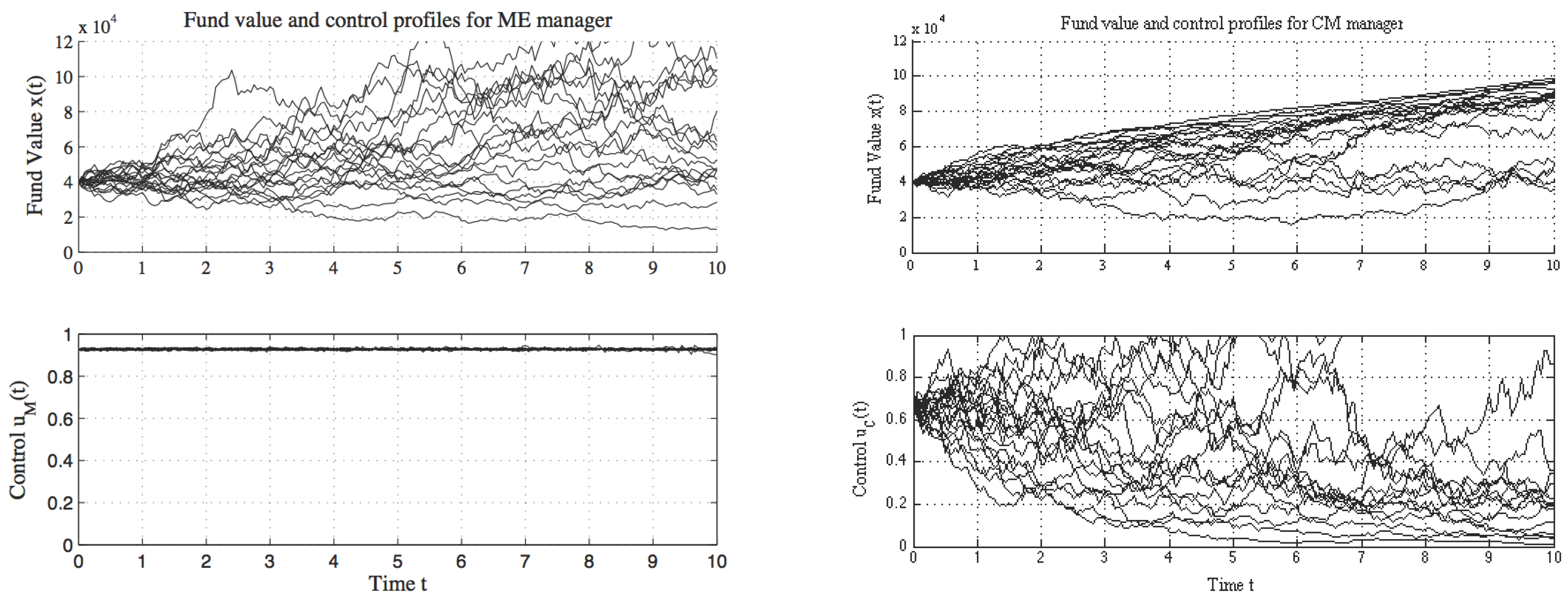
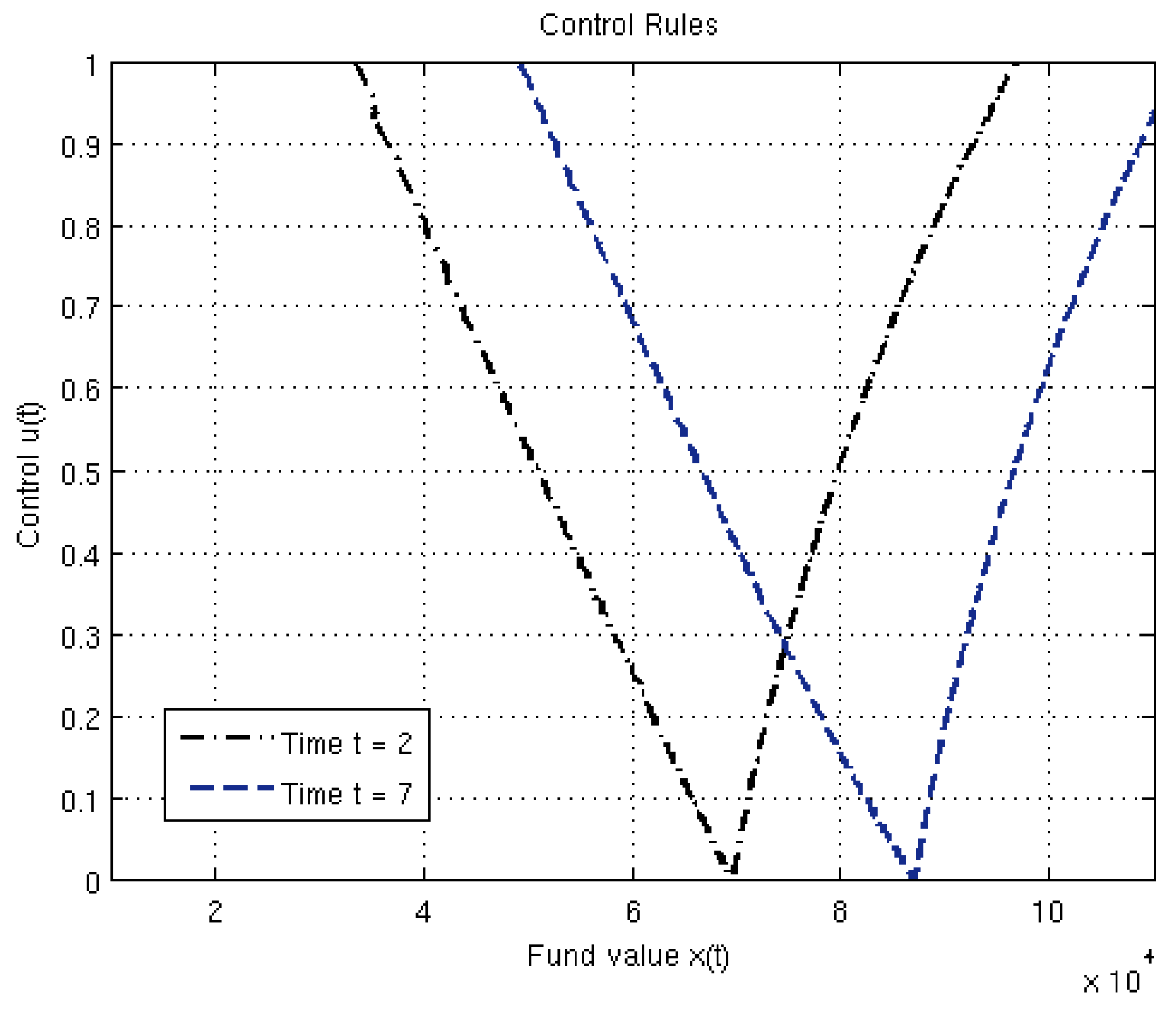
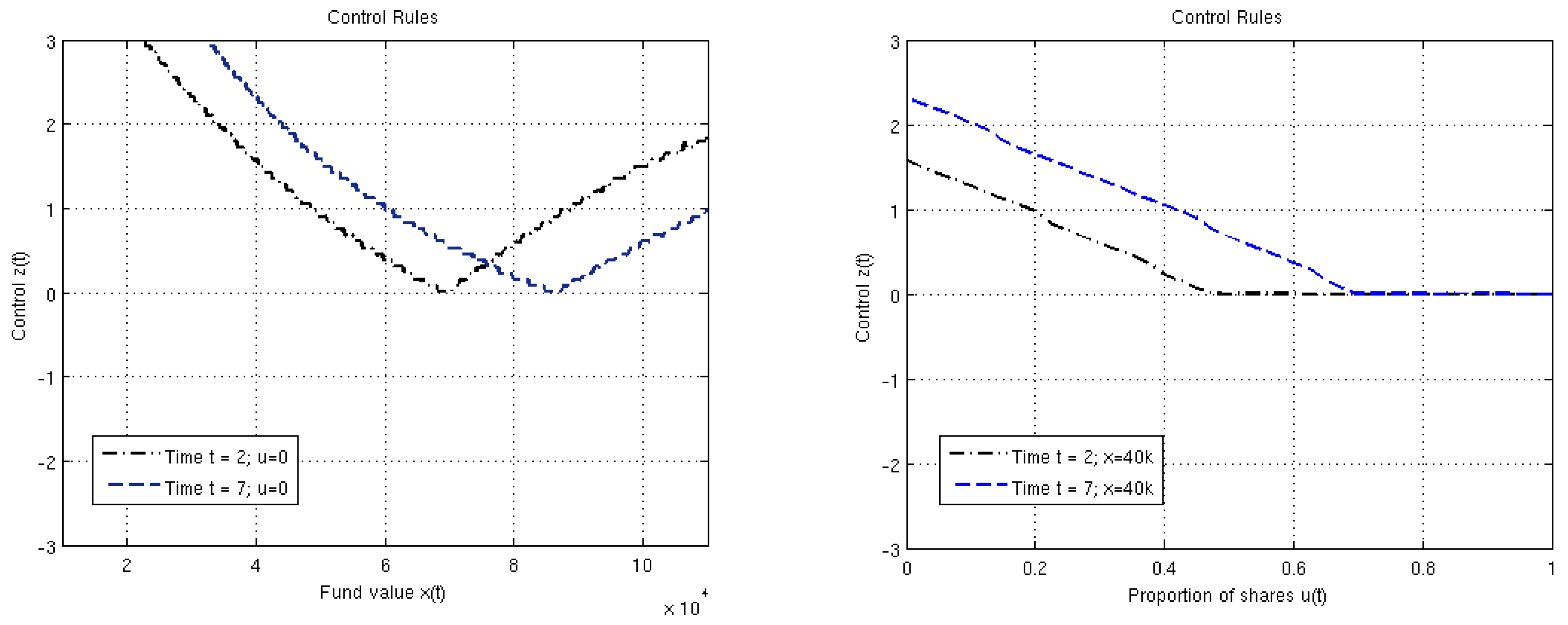
4.1. Optimal strategies

Let μ . ( x , t ) , t [ 0 , T ] denote a strategy for keeping an optimal proportion of shares. This strategy maps an observation x ( t ) at time t into the optimal number of shares u ( t ) . (We claim that wealth x ( t ) is more natural upon which to build a useable feedback strategy than state price density as in [22].) To establish the optimal strategy with b = 0 , an investor will solve the following optimal control problem:
μ . ( x , t ) = arg max ( 9 ) subject to ( 5 ) and ( 3 ) .
The Merton-optimal strategy for the proportion of shares, μ M ( x ) , which does not depend on t (see e.g., [18]), can be established through (10) with h ( · ) in (9) replaced by (8). A cautious-relaxed investor will seek μ M ( x , t ) through (10) with h ( · ) in (9) replaced by (7).
As said in the introduction, the Merton strategy μ M ( x ) can be analytically established (see Appendix C) while the cautious-relaxed μ C ( x , t ) has been obtained numerically15 by the specialised software SOCSol from [12] (also, see [28]).
We will calculate the optimal strategy μ C ( x , t ) for a parametrised pension management problem, described in Appendix A. Briefly, the initial outlay is x 0 = $ 40 , 000 and is to be managed for T = 10 years. If the volatility from the risky asset was eliminated and only the drift remained then $40,000 would grow to $89,021.63 in 10 years (see (13)). Rounded up, this yields $100,000 which was selected as the pension-reference level x T , not too easily obtained.
The strategies that solve a portfolio-investment problem of a cautious-relaxed investor with b = 0 are shown in Figure 2. The vertical axis is u ( t ) , the proportion of wealth to be invested into shares and the horizontal axis is the level of wealth x ( t ) . The strategies are feedback (see [11]), they change with time and state (wealth). It seems intuitive that an investor would adjust their allocations with performance. For example, if an investor’s fund is performing poorly, the investor would be well advised to shift their investment towards more risky investments in order to at least have the chance of recouping losses. This is different to the application of a flat strategy obtained for the Merton investor, see (21) in Appendix C.
Figure 2. Control rules for x T = $ 100 , 000 and t = 2 , t = 7 .
Risks 03 00318 g002
In more detail, we notice that the investment minimum, which occurs in this figure at u = 0 , defines two investment zones.
(1) Fund values x ( t ) ( 0 , x S ( t ) ) where x S ( t ) is where u = 0 . In this zone, the pension reference level x T can only be reached by investing in the risky asset. Here, the investor must gamble to evade heavy penalties for falling short of x T .
(2) Fund values x ( t ) > x S ( t ) , from which x T can be reached by investing solely in the secure asset. In this zone, the investor strives to maximise their reward for exceeding x T , which is a less aggressive process than in the first zone because κ ( 0 , 1 ) in this zone (see (7)).
As said, the investor is relaxed about exceeding the reference level x T . If the fund value is such that x T can be reached by investing all wealth in the secure asset, committing a fixed minimal portion of x ( T ) (e.g., $100) to the shares could, for large volatilities, result in a negative expected yield. Hence, if investment cannot be made smaller than a predetermined number of shares, then the zero investment ( u ( t ) = μ ( x S , t ) = 0 ) may dominate this fixed minimal portion investment. For some details, see Appendix D.
In Figure 3 a random selection of 20 (out of 100,000 used to generate Figure 4) time profiles of the fund values and the strategy realisations for t [ 0 , T ] [ 0 , 10 ] are shown for a Merton investor (“ME" - left panels) and a cautious-relaxed investor (“CM" - right panels). The strategy realisations u C ( t ) (in the right bottom) are jerky (see [11]) as opposed to Merton’s which appear flat.16 This implies that a cautious-relaxed investor will have to rebalance their portfolio very frequently, and expensively if b is large. The shares’ exposure adjustments of the Merton investor are evidently much smaller.
Figure 3. Fund value and strategy realisations.
Risks 03 00318 g003

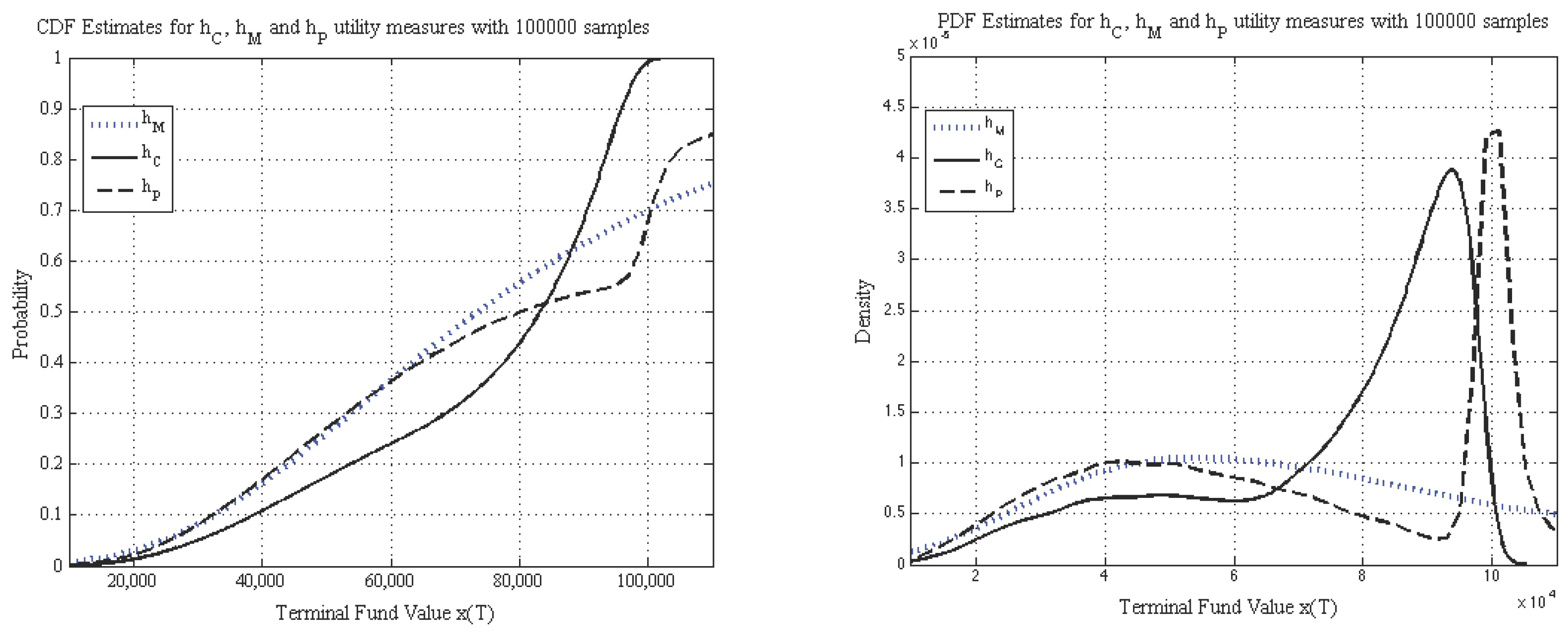
4.2. Pension distributions

Figure 4 shows three pension payoff distributions, cumulative in the left panel and probability in the right panel. The distributions are obtained for a parameterised pension management problem, defined in Appendix A; in particular the reference payoff x T = $ 100 , 000 . The distributions for h M (the blue dotted lines) were derived analytically as a result of applying the optimal Merton investment strategy (see Appendix C). The solid lines correspond to the simulated payoffs obtained as outcomes of the cautious-relaxed strategy, see [15]. The dashed lines are payoff distributions for a strategy that maximises the prospect-theoretic function h P , shown in Figure 1. The last two distributions are obtained by using the respective strategy 100,000 times and measuring the obtained payoffs.
Figure 4. Fund value cumulative and probability distributions.
Risks 03 00318 g004
Both panels tell the same story because they refer to the same distributions. We show both because some distribution features such as quantiles are easier to demonstrate on the cdf graphs, while others such as modes are easier to illustrate on the pdfs. The summary statistics for the Merton and cautious-relaxed pension distributions are presented in Table 1. (For convenience of comparisons with the pensions with transaction costs, most of them are repeated in Table 2.)
Table 1. Merton and cautious-relaxed pension yield distribution statistics.
StatiticCaut.-Relax.Merton
Mode of x ( 10 ) $93,790$55,300
Mean of x ( 10 ) $74,922$86,596
Median of x ( 10 ) $83,373$73,082
Std. dev. of x ( 10 ) $21,723$55,042
Coeff. of skew.–1.0172.164
P ( x ( 10 ) > $ 105 , 000 ) 00.273
P ( x ( 10 ) > $ 80 , 000 ) 0.5620.438
P ( x ( 10 ) < $ 40 , 000 ) 0.10770.15
The h M (Merton’s) yield distribution is log-normal and right-skewed with the mode below $60,000. The probability of achieving a yield better than $105,000 is about 0.27. The median is $73,082 which is less than the mean $86,596. The probability of attaining less than $40,000, which is the initial outlay in our parametrised problem, is about 0.15 and the probability of reaching a pension above $80,000 is 0.438. The corresponding numbers for the h C yield distribution (cautious-relaxed) are as follows. The probability of achieving a yield better than $105,000 is 0; the median is $83,343, which is more than the mean $75,228. The probability of attaining less than $40,000 is about 0.11 and the probability of reaching a pension above $80,000 is 0.562. The numerical measure of skewness17 indicates a large difference between the Merton’s and cautious-relaxed distributions.
We do not list the numerical values for the prospect-theoretic distribution h P (dashed lines), which are in-between the Merton’s and cautious-relaxed. The fact that h P ’s mode dominates the one corresponding to h C is obvious; however, the probability of scoring a payoff greater than $80,000 is higher for the cautious-relaxed pension, which – in our view – lessens the attractiveness of a prospect-theoretic distribution for pension optimisers.
The comparisons of the probabilities of a disastrous yield below the initial outlay and those of a yield above $80,000 clearly point to h C as the utility measure that a pension optimiser will favour.
In the next section, the impact of a transaction cost on the skewness of the terminal fund value distribution will be examined.

5. Cautious-relaxed strategies and pension distributions with transaction costs

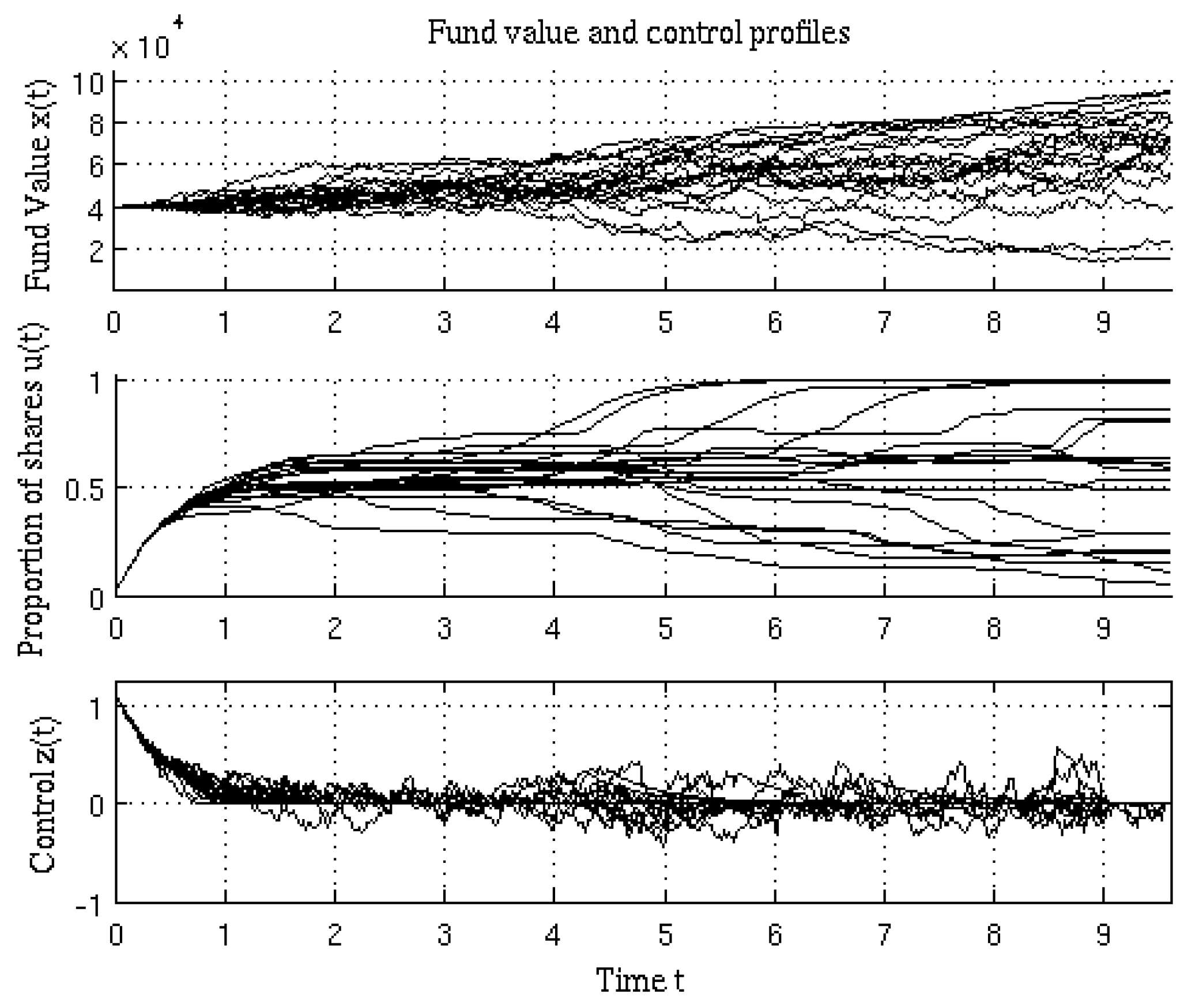
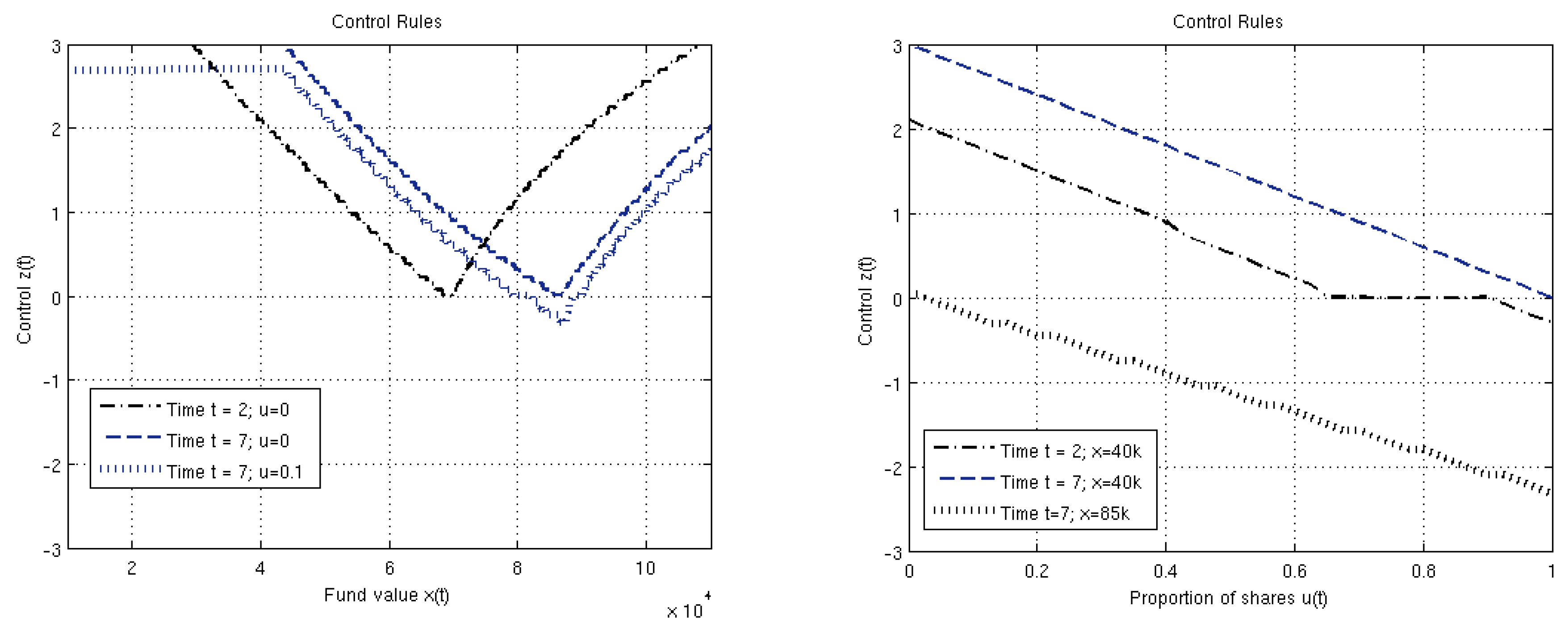
5.1. Optimal strategies

Let ζ ( x , u ) denote a strategy for an optimal share exposure’s corrections, or portfolio rebalancing. (So z ( t ) , see (4), is a realisation of strategy ζ ( x ( t ) , u ( t ) ) at time t.) The cautious-relaxed investor now solves this optimal control problem:
ζ ( x , u ) = arg max ( 9 ) subject to ( 4 ) , ( 5 ) and ( 3 )
with b > 0 and h ( · ) as in (7).
The computed cautious-relaxed strategies for b = 0 . 005 and b = 0 . 05 are displayed in Figure 5 and Figure 6, respectively. Strategies and their outcomes for more values of b are commented on in Table 2.
Figure 5 shows a sample of the strategies for a “small" transaction cost. The left panel shows them as functions of wealth x ( t ) and the right panel – as functions of the proportion of wealth invested in shares u ( t ) . These strategies tell the investor which adjustment z ( t ) needs to be made to the current proportion of shares u ( t ) , given wealth x ( t ) . In other words, a value of z ( t ) says by which proportion of wealth the number of shares needs to be altered in a period (so, z ( t ) are rates); here, the period length is Δ = 1 / 3 .
Suppose the investor’s wealth in time 2 is x ( 2 ) = $ 40 , 000 and no shares are owned so, u ( 2 ) = 0 . Figure 5 recommends (see the dash-dotted line),
z ( 2 ) = ζ ( x ( 2 ) , 0 ) · Δ = 2 . 1 · 1 / 3 = 0 . 7 .
This value is less than (but still quite close to) 0.79, which Figure 2 tells us is the corresponding investment into shares at t = 2 when there are no transaction fees.
Figure 5. Control rules for t = 2 and t = 7 in x ( t ) (left panel) and u ( t ) (right panel) for b = 0 . 005 .
Risks 03 00318 g005
Now, suppose that the investor’s wealth at t = 7 is $85,000. Figure 2 advises u ( x ( 7 ) ) = 0 . 038 as optimal when there are no transaction costs. Suppose that at this time 10% of the investor’s wealth is in shares. In Figure 5, we can read (see the dotted line) that the exposure needs to diminish by
z ( 7 ) = ζ ( x ( 7 ) , 0 . 1 ) · Δ = - 0 . 225 · 1 / 3 = - 0 . 075 .
So, u ( 7 ) = 0 . 1 - 0 . 075 = 0 . 025 . This is less than 0.038, the shares’ exposure when there are no transaction costs.
The above two numerical examples suggest that charging the shares’ updates b = 0 . 005 per period dampens the investor’s behaviour.
Consider now a higher cost ( b = 0 . 05 ). Figure 6 shows ζ ( x ( t ) , u ( t ) ) projected into z ( t ) , x ( t ) and z ( t ) , u ( t ) in the left and right panels, respectively. The strategies are flatter than in Figure 5, which means that smaller adjustments are recommended. In particular, for x ( 2 ) = $ 40 , 000 and if the original number of shares is zero, Figure 6 recommends (see the dash-dotted line)
z ( 2 ) = ζ ( x ( 2 ) , 0 ) · Δ = 1 . 575 · 1 / 3 = 0 . 525 ,
which is less than than 0.7, optimal when b = 0 . 005 . As the value of the original number of shares was zero, z ( 2 ) = 0 . 525 is the number of shares to buy. This is obviously less than 0.79 when b = 0 , read from Figure 2. Evidently, the investor restrains not only their share-adjustment size but also the risky asset exposure.
Figure 6. Control rules for t = 2 and t = 7 in x ( t ) and u ( t ) for b = 0 . 05 .
Risks 03 00318 g006
Figure 7. Sample of fund value, proportion of shares and shares’ adjustments for b = 0 . 01 .
Risks 03 00318 g007
Figure 7 shows a sample of realisations of fund value, proportion of shares and shares’ adjustments for an even higher (than in Figure 6) transaction cost b = 0 . 01 . A casual comparison of the first two panels in this figure to Figure 3’s clearly documents that this transaction cost dampens the jerky behaviour of shares’ exposure corrections, (almost) without affecting the desirable yield’s clustering in the top of its graph. It will be interesting to see if the left-skewness of the pension distribution for this cost will be preserved.

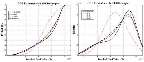
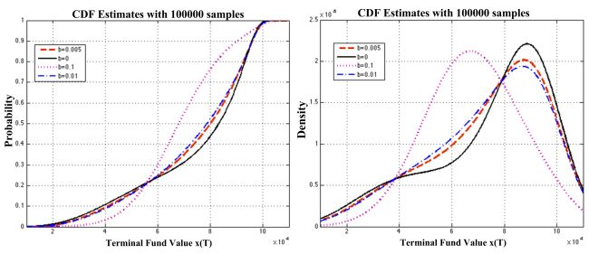
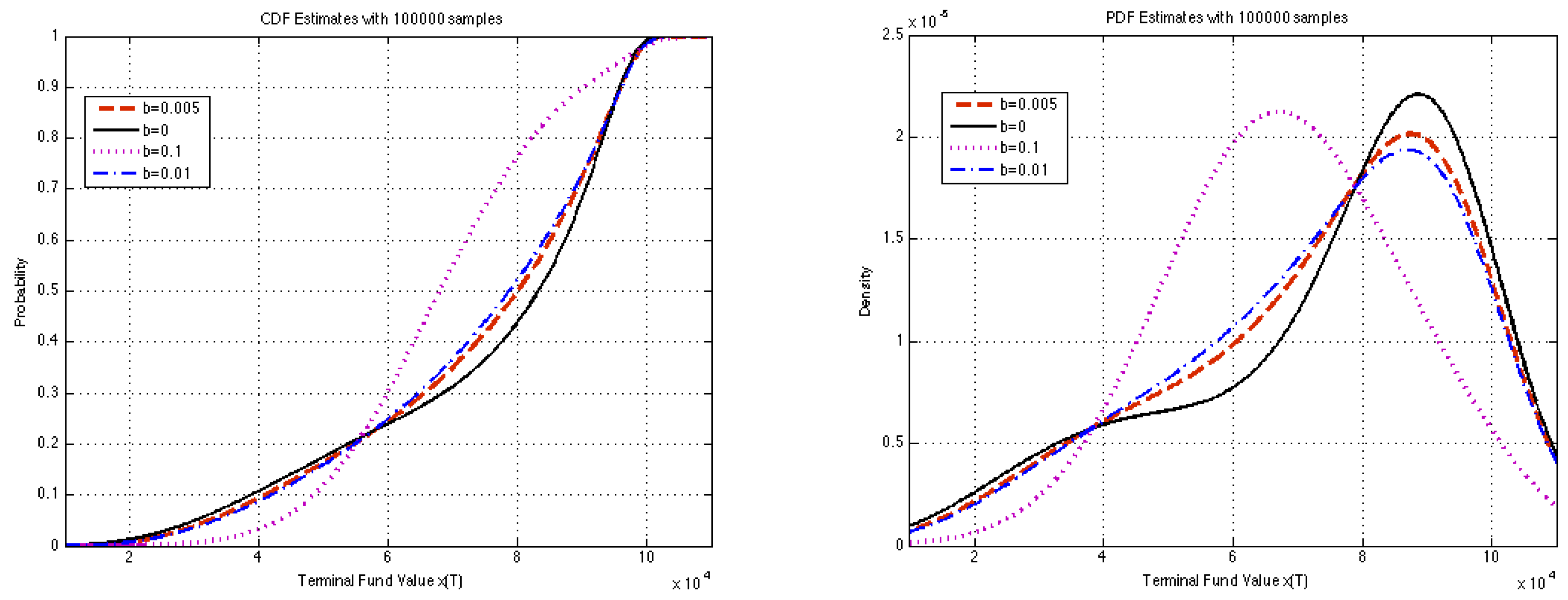
5.2. Pension Distributions

We will now see if the restrained share updating behaviour has an impact on the left-skewness of the pension yield.
The solid black cdf in Figure 8 (in the left panel) is the pension distribution for no transaction costs, which is the same distribution as shown in Figure 4. As documented by the dashed (red) and dash-dotted (blue) lines, for small and median transaction costs ( b = 0 . 005 and b = 0 . 01 ), the left-skewness of the pension yield distributions is preserved. The dotted line is for b = 0 . 1 and looks almost symmetric, This clearly demonstrates that the left-skewness is lost for high costs.
Figure 8. Fund value cumulative and probability distribution functions for various values of b.
Risks 03 00318 g008
Table 2. Pension distributions statistics.
Statistic b = 0 b = 0.005 b = 0.01 b = 0.05 b = 0.1 Merton
Mean of x ( 10 ) $74,922$74,000$73,657$70,651$68,493$86,596
Median of x ( 10 ) $83,373$80,133$78,815$71,297$67,966$73,082
Std. dev. of x ( 10 ) $21,723$20,741$20,464$18,108$15,640$55,042
Coeff. of skew. of x ( 10 ) –1.017–0.8499–0.78–0.3310.01582.164
P ( x ( 10 ) > $ 80 , 000 ) 0.5620.5030.4750.3330.2330.438
P ( x ( 10 ) < $ 40 , 000 ) 0.10770.09380.08750.05610.03170.15
Examine Table 2, which provides aggregate statistics on the pension yield distributions for several transaction cost rates. The column marked ’ b = 0 ’ gives the numbers for the costless caution-relaxed strategy from Section 4. The last column is for the classic Merton strategy (21) without transaction costs.
As expected, the higher a transaction cost, the lower the mean and median of the pension yield. Standard deviations also decrease as the costs grow, which indicates smaller variability of the yield for higher charges. Medians dominate means but their differences become small, which is evidence of the distributions’ symmetrisation. The numerical measure of skewness also indicates increasing symmetrisation.
The last two rows of Table 2 provide measures of how well a strategy scores on the main two features of cautious-relaxed strategies: a high probability of yields proximate to the reference position x T and a (probabilistic) guarantee of low losses. We can see that charging b = 0 . 01 and less, delivers distributions where obtaining x ( T ) $ 80 , 000 is at least 0.475, which is more than using the Merton strategy (see last column). The low probability of losses ( x ( T ) $ 40 , 000 ) is obtained for all cautious-relaxed strategies. However, higher charges than b = 0 . 01 make a cautious-relaxed strategy unattractive because of the decreasing mean and a small probability of approaching the reference pension.

5.3. Advice

A question might be asked how high the transaction costs may be in “real-life". In the parametrised problem, the rates in equation (5) are expressed in annual terms. We have read in Figure 5 and Figure 6 that the z-values for x ( 2 ) = $ 60 , 000 and u ( 2 ) = 0 are 0.6 and 0.45 for b = 0 . 005 and b = 0 . 05 , respectively. So, correspondingly, the trimester charges for these values of b would be 0 . 005 · 4 / 12 · 0 . 6 · $ 60 , 000 = $ 60 and 0 . 05 · 4 / 12 · 0 . 45 · $ 60 , 000 · 4 = $ 450 .
As a “rule of thumb”, our investor should use cautious-relaxed strategies if an annual cost aggregates to less than $500, which would roughly correspond to b = 0 . 01 .

6. Conclusion

This paper performs a further analysis of issues raised in [11] involving cautious-relaxed investment strategies obtained as optimal solutions to a stochastic optimal control problem of pension portfolio management. It was shown there that a non-gambling investor can find left-skewed payoff distributions favourable that result from a utility measure kinked around a payoff reference point. However, the underlying cautious-relaxed investment strategy realisations were jerky, which might have been due to the absence of transaction costs. In this paper a sensitivity analysis of the cautious-relaxed strategies to transaction costs has been performed. It has been found out that realistic costs can mitigate the jerkiness without destroying the pension yield distribution’s left-skewness. For high transaction charges, using the classic Merton strategy becomes attractive.
The above results allow us to propose that payoff distributions are important determinants of advantages between various investment strategies obtained as maximisers of some utility measures. As many distributions are analytically intractable the proposed approach, which is scalable to more complex models, should be of interest to funds’ managers.

Acknowledgments

I am indebted to Wilbur Townsend for insightful comments and editorial suggestions and to Vlad Gaitsgory for a discussion on “fast" controls. I am also very grateful to three anonymous referees for their constructive comments and to the academic editor of this journal for final advice. All remaining errors are mine.

Conflicts of Interest

The author declares no conflict of interest.

A. Parameters

As stated in the introduction, our solutions are numerical and, hence, parameter specific (yet scalable to more complex models). The hypothetical base-case scenario that we study involves an initial outlay x 0 = 40 , 000 invested in a pension fund to be collected as a lump sum after T = 10 years. Table 3 shows the rest of the parameters that are utilised in this study.
Table 3. Selected Parameters
rασc
0.050.0850.2.005
With these parameters the fund will accumulate to
$ 40 , 000 e ( r - c ) T = $ 40 , 000 e ( 0 . 05 - . 005 ) 10 = $ 62 , 732 . 49
if all money is invested in the risk-free asset. This figure can be referred to as the guaranteed amount. It should be expected that a pension fund investor would require the pension yield to regularly surpass this value.
However, if the volatility from the risky asset was eliminated and only the drift remained then $40,000 would grow to
$ 40 , 000 e ( α - c ) T = $ 40 , 000 e ( 0 . 085 - 0 . 005 ) 10 = $ 89 , 021 . 63
in 10 years.

B. SOCSol and Yield Distributions

Due to the non-symmetric and non-smooth nature of the cautious-relaxed investor’s utility measure, an analytical solution to the investment problem is not available at this stage. We have resolved this by generating the optimal investment strategies using a program called SOCSol, developed in Matlab and introduced in [29]. The program discretises optimal control problems and solves them using Markov Chains. See [12] and [13] for more details on SOCSol.
Different wealth-path realisations are generated within SOCSol using Monte Carlo simulation for a given optimal investment strategy. The distributions of wealth at time T are obtained numerically by analysing the generated realisations of x ( T ) .

C. The Merton Investor

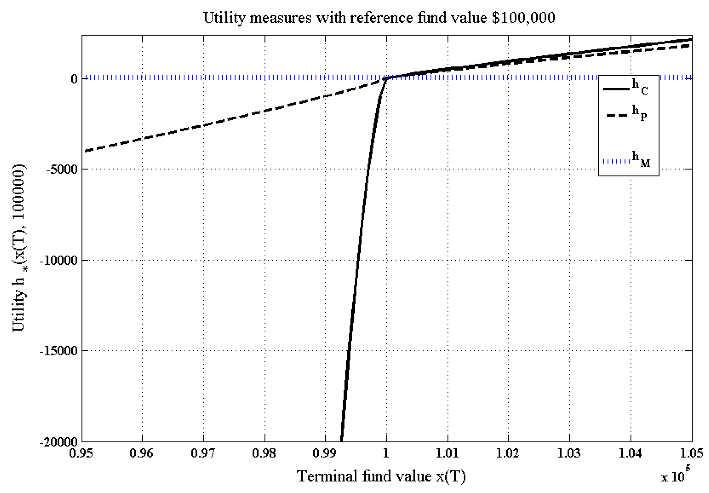
C.1. The Classic Utility Measure

An expected value of a concave utility function is the classic portfolio performance measure, see [4] and [30]. We will present the (known) optimal investment strategy and analyse the resulting payoff distribution.
The choice of h ( x ( T ) ) in (6) is now the issue of concern. The classic Merton investor will use the concave utility function (8) (compare [18]). Analytically, the optimal solution to their problem can easily be found as a solution to the Hamilton-Jacobi-Bellman equation. First, we define a value function for the portfolio problem:
V ( t , x ) = sup u J ( x ( t ) , u )
where J ( · , · ) is expected utility as in (9). This gives the following Hamilton-Jacobi-Bellman equation:
max 1 2 u ( t ) 2 σ 2 x 2 V x x ( t , x ) + ( r + u ( t ) ( α - r ) - c ) x ( t ) V x ( t , x ) + V t ( t , x ) = 0
with boundary condition
V ( T , x ) = 1 δ x δ .
Maximisation of (15) gives
u ( t ) = - α - r σ 2 V x ( t , x ) x V x x ( t , x )
substituting into the Hamilton-Jacobi-Bellman equation (15) implies
0 = - 1 2 ( α - r ) 2 σ 2 V x 2 ( t , x ) V x x ( t , x ) + ( r - c ) x ( t ) V x ( t , x ) + V t ( t , x ) .
The boundary condition set by (16) suggests the functional form for V ( t , x ) :
V ( t , x ) = f ( t ) 1 δ x δ , f ( T ) = 1 ;
plugging this into (18) we are left with an ordinary differential equation
0 = δ 1 2 ( α - r ) 2 σ 2 ( 1 - δ ) + ( r - c ) f ( t ) + f ( t ) .
This ODE is easily solved with a solution f ( t ) = e δ ( r - c ) + ( α - r ) 2 2 σ 2 ( 1 - δ ) ( T - t ) implying that (19) is the correct guess of the value function. Substituting this value function into (17) gives
u ( t ) = α - r σ 2 ( 1 - δ ) ,
which is the known “flat" optimal solution to the Merton investor’s problem (e.g., see [18]).
The same proportion of wealth is always invested into the risky and risk-free asset. This seems to be quite unintuitive in that you would expect an investor to change their strategy in order to adjust to the performance of the portfolio. Some rebalancing of the portfolio will still be needed to maintain the constant (21) but the corresponding transaction cost will be small.

C.2. The Distribution

While the cumulative and probability distributions for cautious-relaxed strategies are analytically non-tractable (and obtained numerically in this paper), the Merton payoff distribution shown as the (blue) dotted line in Figure 4 can be obtained in closed form.
We find18 that after fitting the optimal control (22) to the state equation (5), wealth x ( t ) is a Geometric Brownian Motion that follows
d x ( t ) = M x ( t ) d t + Σ x ( t ) d w
where M = ( r - α ) 2 ( 1 - δ ) σ 2 + r - c and Σ = α - r σ ( 1 - δ ) . This means that for an initial value x 0 , wealth x ( t ) t ( 0 , T ] is a log-normally distributed random variable with expected value
M ̲ ( t ) E ( x ( t ) ) = e M t x 0
and variance
Σ ̲ 2 ( t ) Var ( x ( t ) ) = e 2 M t x 0 2 e Σ 2 t - 1 .
We also know that the wealth is the stochastic process
x ( t ) = x 0 exp M - Σ 2 2 t + Σ w ( t ) , t [ 0 , T ] .
Finally, the probability density function of wealth x ( T ) is log-normal:
f X T ( x ; M ̲ T , Σ ̲ T ) = 1 x Σ ̲ T 2 π T exp - ( ln x - ln x 0 - T ( M ̲ T - 1 2 Σ ̲ T 2 ) ) 2 2 Σ ̲ T 2 T , x > 0
where M ̲ T , Σ ̲ T are M ̲ ( t ) , Σ ̲ ( t ) evaluated at t = T .
We know that a log-normal distribution is generically non-symmetric (which, in our view, causes a problem of using strategy (21) by an investor seeking to avoid large losses) .
Substituting the values given in Table 3 to the Merton solution given in (21) and using a δ = 0 . 05 gives an optimal u ( t ) of 0.921. This means that 92.1% of wealth at any time is invested in the risky asset. Now that all the respective parameters have been set, we can evaluate the mean, variance and other statistics using the formulae given above, see Table 2.
The Merton investment strategy provides the distribution of payoffs shown as the (blue) dotted line in Figure 4. We see that the payoff is right skewed with relatively high probabilities of being below the original investment and of being below the guaranteed amount, all analysed in Table 2.

D. Why Zero-Investment Can Be Profitable in This Model

It is important to note that some levels of wealth, which we denote x S ( t ) , will virtually generate no investment in the risky asset. This will happen when the reference level payoff x T can be obtained without the risky asset and if the risky-asset investment brings an expected value that is less than the secure investment. For example if at time 6, x ( 6 ) = $ 83 , 527 , then u ( τ ) 0 for τ [ 6 , T ] . This is because $ 83 , 527 e ( 0 . 05 - 0 . 005 ) ( 10 - 6 ) = $ 100 , 000 so, x T is obtainable without the risky asset. For the relatively high volatility ( σ = 0 . 2 ), the risky-asset investment of the size compatible with the adopted grid size (or constrained by a minimal investment), brings an expected value of marginal utility that is less than the secure gain and all funds19 will be allocated to the risk-free asset. We can say that wealth at time 6 has reached the secure-investment level x S ( 6 ) . Using u ( τ ) = 0 for τ 6 from x S ( 6 ) causes every x ( τ ) to the right of the x-intercept of the strategy graph in Figure 2, to be reached at the right time for the investor to continue the strategy u ( x S ( τ ) ) = 0 .

References

  1. T. Bali, N. Cakici, and R. Whitelaw. “Maxing out: Stocks as lotteries and the cross-section of expected returns.” J. Financ. Econ. 99 (2011): 427–446. [Google Scholar] [CrossRef]
  2. N. Barberis, and M. Huang. “Stocks as Lotteries: The Implications of Probability Weighting for Security Prices.” Am. Econ. Rev. 98 (2008): 2066–2100. [Google Scholar] [CrossRef]
  3. P. Brockett, and Y. Kahane. “Risk, Return, Skewness and Preference.” Manag. Sci. 38 (1992): 851–866. [Google Scholar] [CrossRef]
  4. R.C. Merton. “Optimum consumption and portfolio rules in a continuous-time model.” J. Econ. Theory 3 (1971): 373–413. [Google Scholar] [CrossRef]
  5. M. Annunziato, and A. Borzì. “Optimal control of probability density functions of stochastic processes.” Math. Model. Anal. 15 (2010): 393–407. [Google Scholar] [CrossRef]
  6. C. Bernard, J.S. Chen, and S. Vanduffel. “Rationalizing investors’ choices.” J. Math. Econ. 59 (2015): 10–23. [Google Scholar] [CrossRef]
  7. J. Outreville. “Meaning of Risk.” Geneva Pap. Risk Insur. Issues Pract. 39 (2014): 768–781. [Google Scholar] [CrossRef]
  8. B. Jacobs, and K. Levy. “Traditional Optimization Is Not Optimal for Leverage-Averse Investors.” J. Portf. Manag. 40 (2014): 30–40. [Google Scholar] [CrossRef]
  9. D. Goldstein, E. Johnson, and W. Sharpe. “Choosing Outcomes versus Choosing Products: Consumer-Focused Retirement Investment Advice.” J. Consum. Res. 35 (2008): 440–456. [Google Scholar] [CrossRef]
  10. X. He, and X. Zhou. “Portfolio choice via quantiles.” Math. Finance 21 (2011): 203–231. [Google Scholar] [CrossRef]
  11. J.B. Krawczyk. “On loss-avoiding payoff distributions in a dynamic portfolio management problem.” J. Risk Finance 9 (2008): 151–172. [Google Scholar] [CrossRef]
  12. J.D. Azzato, and J.B. Krawczyk. “Parallel SOCSol: A Parallel MATLAB (R) package for approximating the solution to a continuous-time stochastic optimal control problem.” Technical report, Victoria University of Wellington. 2008. Available online: http://researcharchive.vuw.ac.nz/handle/10063/387 (accessed on 18 August 2015).
  13. J.B. Krawczyk. “Numerical Solutions to Lump-Sum Pension Fund Problems That Can Yield Left-Skewed Fund Return Distributions.” In Optimal Control and Dynamic Games. Edited by C. Deissenberg and R.F. Hartl. Dordrecht, The Netherlands: Springer, 2005, Chapter 11; pp. 155–176. [Google Scholar]
  14. J. Foster. “Target Variation in a Loss Avoiding Pension Fund Problem Problem.” Technical report, Victoria University of Wellington. 2011. Available online: http://mpra.ub.uni-muenchen.de/36177/1/writeup.pdf (accessed on 18 August 2015).
  15. J. Azzato, J. Krawczyk, and C. Sissons. “On loss-avoiding lump-sum pension optimization with contingent targets.” Working Paper Series 1532, Victoria University of Wellington, School of Economics and Finance. 2011. Available online: http://EconPapers.repec.org/RePEc:vuw:vuwecf:1532 (accessed on 18 August 2015).
  16. J.B. Krawczyk. “A Markovian approximated solution to a portfolio management problem.” Inf. Technol. Econ. Manag. 2001. Available online: http://personal.victoria.ac.nz/jacek_krawczyk/somepapers/portfitem.pdf (accessed on 20 August 2015).
  17. J. Foster, and J.B. Krawczyk. “Sensitivity of Cautious-Relaxed Investment Policies to Target Variation.” Working Paper Series 1532, Victoria University of Wellington, School of Economics and Finance. 2013. Available online: http://EconPapers.repec.org/RePEc:vuw:vuwecf:1532 (accessed on 18 August 2015).
  18. W.H. Fleming, and R.W. Rishel. Deterministic and Stochastic Optimal Control. New York, NY, USA: Springer, 1975. [Google Scholar]
  19. V. Gaitsgory. “Suboptimization of singularly perturbed control systems.” SIAM J. Control Optim. 30 (1992): 1228–1249. [Google Scholar] [CrossRef]
  20. D. Blake. “Portfolio choice models of pension funds and life assurance companies: Similarities and differences.” Geneva Pap. Risk Insur. Issues Pract. 24 (1999): 327–357. [Google Scholar] [CrossRef]
  21. V. Gaitsgory. “Averaging and near viability of singularly perturbed control systems.” J. Convex Anal. 13 (2006): 329–352. [Google Scholar]
  22. A.B. Berkelaar, R. Kouwenberg, and T. Post. “Optimal Portfolio Choice Under Loss Aversion.” Rev. Econ. Stat. 86 (2004): 973–987. [Google Scholar] [CrossRef]
  23. K.F.C. Yiu. “Optimal portfolios under a value-at-risk constraint.” J. Econ. Dyn. Control 28 (2004): 1317–1334. [Google Scholar] [CrossRef]
  24. E. Bogentoft, H.E. Romeijn, and S. Uryasev. “Asset/Liability management for pension funds using CVaR constraints.” J. Risk Finance 3 (2001): 57–71. [Google Scholar] [CrossRef]
  25. H. Jin, and X.Y. Zhou. “Behavioral portfolio selection in continuous time.” Math. Finance 18 (2008): 385–426. [Google Scholar] [CrossRef]
  26. A. Tversky, and D. Kahneman. “Advances in prospect theory: Cumulative representation of uncertainty.” J. Risk Uncertain. 5 (1992): 297–323. [Google Scholar] [CrossRef]
  27. M. Ammann. “Return guarantees and portfolio allocation of pension funds.” Financ. Mark. Portf. Manag. 17 (2003): 277–283. [Google Scholar] [CrossRef]
  28. J.D. Azzato, and J.B. Krawczyk. “Applying a finite-horizon numerical optimization method to a periodic optimal control problem.” Automatica 44 (2008): 1642–1651. [Google Scholar] [CrossRef] [Green Version]
  29. A. Windsor, and J.B. Krawczyk. “A MATLAB Package for Approximating the Solution to a Continuous-Time Stochastic Optimal Control Problem.” 1997. Available online: http://papers.ssrn.com/soL3/papers.cfm?abstract-id=73968 (accessed on 18 August 2015).
  30. P.A. Samuelson. “Lifetime portfolio selection by dynamic stochastic programming.” Rev. Econ. Stat. 51 (1969): 239–246. [Google Scholar] [CrossRef]
  31. P.E. Kloeden, and E. Platen. Numerical Solution of Stochastic Differential Equations. Berlin, Germany: Springer-Verlag, 1992. [Google Scholar]
  • 1(1) When the mass of the distribution is concentrated on the left and the right tail is longer, the distribution is said right- or positively skewed; (2) when the mass of the distribution is concentrated on the right the left tail is longer, the distribution is said left- or negatively skewed.
  • 2Interestingly, in the context of static portfolio management, [8] also question the wisdom of “traditional optimisation" for some investors, leverage-averse in their case.
  • 3Exceptions to this include [9], [10]. The work done on the distribution builder in the first, enables subjects to build their desired pension distribution subject to a budget constraint. However, the results lead to distributions that are right skewed, which could be due to the setting of a (low) reference point at the amount guaranteed by the risk-free asset. In [10], quantiles are proposed as an effective way to evaluate the success and failings of a portfolio.
  • 4Finding analytic solutions to the resulting PDEs would be a substantive research project which may not yield any results as the study subject are nonlinear PDEs. A “semi" analytic solution could be obtained by a functional expansion. We pursue numerical solutions in this paper, which are reliable and easy to interpret for parameter-specific problems.
  • 5Notwithstanding the obtained solution’s parameter-specificity, our analysis can be extended to other cases through the use of specialised software (see [12]).
  • 6Also [13], [14], [15] and [16] .
  • 7This will be a synthetic aggregate good if there are many risky assets.
  • 8Constraint (3) means no short selling or borrowing. This restriction has been weakened in the literature; however, it may be reasonable to keep it in a situation of a pension fund investor.
  • 9A study of the impact of management incentives on investment strategies performed in [17] reports that maximising management revenue from fees changes little the investment strategies.
  • 10An argument for using z ( t ) as control instead of u ( t ) can be found in [21]. If u ( · ) – the “fast" control – is Lebesgue measurable, Proposition 3.2 in that publication establishes that a solution x ( t ) to a differential equation which contains u ( t ) , but not z ( t ) , can be approximated by a solution obtained from an equation where z ( t ) is introduced as in (4).
  • 11This publication deals with portfolio choice models for both pension funds and life assurance companies on a macro scale i.e., where many investors contribute to the fund. In that sense, our one-pension management problem is micro.
  • 12Other constraints could be added, e.g., x ( t ) 0 .
  • 13This measure (7) was also used in, among others, [16], [13] and [17]. A loss-averse utility function that is concave on each side of the reference point (so, “similar" to (7)) was proposed in [22]. However, for the original parameters adopted by [22], that function is only “lightly” concave and did not generate left-skewed distributions, see [15].
  • 14These authors solved the problem by splitting it into subproblems and found that the optimal strategy is one in which the investor takes on aggressive gambling strategies. The strategies computed in [23] and [24] still generate right skewed distributions, which we deem not preferable by pension fund investors.
  • 15The problem with an analytical solution is that the as long as α in the utility measure (7) is just any number greater than 1, little can be said about a closed-form strategies and value functions. This is because t and x in V ( t , x ) (as in (18)) for the boundary problem with V ( T , x ( T ) ) = - ( x T - x ( T ) ) a , a > 1 appear non-separable. Nevertheless, even if V ( x , t ) were obtained in an analytical form, a closed-form for the payoff-density function would still be an open problem. We also note that closed-form solutions in [22] were obtained for a similar but non-identical, utility function. More importantly their independent variable is not the current (observable) wealth but state price density.
  • 16The strategies are constant but some rebalancing is still needed to maintain a constant optimal proportional exposure of the risky asset, see [18] or [17].
  • 17The skewness coefficient is calculated as E X - mean stand . dev . 3 . It provides a measure of asymmetry in the distribution.
  • 18Compare the methods put forward in [31] and [5].
  • 19We can see in [11] that u ( t ) is never zero for less volatile risky assets.

