Abstract
One numerical method was designed to solve the time-dependent, three-dimensional, incompressible Navier–Stokes equations in turbulent thermal channel flows. Its originality lies in the use of several well-known methods to discretize the problem and its parallel nature. Vorticy-Laplacian of velocity formulation has been used, so pressure has been removed from the system. Heat is modeled as a passive scalar. Any other quantity modeled as passive scalar can be very easily studied, including several of them at the same time. These methods have been successfully used for extensive direct numerical simulations of passive thermal flow for several boundary conditions.
1. Introduction
Turbulence is probably the open problem in physics with most applications in daily life. Turbulent flows are intrinsic to almost any flow in engineering, but they are also extremely important in meteorology or the dispersion of contaminants. It is well known that we still even lack an existence and uniqueness theorem about the solution of the governing equations of turbulent flows, the Navier–Stokes equations. Moreover, these equations cannot be solved analytically apart from some trivial examples. It is generally admitted that the simulation can be considered at three levels of detail, Reynolds Average Navier Stokes (RANS), Large Eddy Simulation (LES), and Direct Numerical Simulations (DNS) [1] which also corresponds to different levels of precision. Both RANS and LES models can simulate typical industrial flows with the necessary accuracy and in practical computation times [2,3,4,5], but DNS is until now the only trustworthy method to investigate physical properties of flows which are little understood.
However, DNS are extremely expensive as every scale of turbulence, both temporal and spatial ones, has to be properly resolved. This implies very fine grids and small temporal steps. Moreover, and as a consequence of Kolmogorov’s scales, [6,7], the number of points needed to carry out the simulation grows extremely fast, as , where is the Reynolds number. Thus, to use DNS to understand turbulent flows, very simple geometries are employed, allowing very precise and fast numerical tools that will be described in this paper. Canonical wall-bounded flows are pipes, channel flows, and the flat-plate boundary layer. These flows are in essence theoretical abstractions and do not appear as such in reality. However, they constitute the basic blocks of more complete real flows and have been studied for 80 years. For isothermal flows, experiments of these canonical flows have been instrumental in the development of the theory since the birth of boundary layer research. In particular, they remain important for the study of very high Reynolds numbers, as DNS is still not able to reach Reynolds numbers as high as those of experiments. High Reynolds numbers are needed to obtain a clear separation of scales related to the near-wall turbulence cycle. The main control parameter is the friction Reynolds Number , where is the viscosity, h is a characteristic length and is the friction velocity at the wall. The largest experiment ever done has been published in 2018 for a friction Reynolds number of 2e4 [8], a value that is absolutely out of reach for DNS. That said, simulations of wall-bounded turbulence are particularly helpful in identifying physical processes occurring in near-wall turbulence as the whole velocity field (and its derivatives) is available. Moreover, experiments showing the 3D thermal field of a turbulent flow are almost impossible to do. For thermal flows, DNS can give insight where experimental flows are impossible.
The first wall-bounded simulation was run by Kim, Moin, and Moser in 1987 [9] for channel flows and in 1988 by Spalart [10] for Turbulent Boundary Layers. Since then, the friction Reynolds number simulated has been continuously growing [11,12,13,14,15,16,17,18,19]. Some of these simulations, Refs. [12,16,18,19] were made with an earlier version of this code. The history is similar for thermal passive flows, but the Reynolds number reached grew up at a slower pace. The first DNS of a thermal flow was carried out by Kim and Moin in 1987 [20]. Kim and Moin obtained first-order turbulence statistics for and several Prandtl numbers, 1 and 2. The Prandtl number is the ratio between momentum diffusivity to thermal diffusivity. They also computed a very important number for modeling, the turbulent Prandtl number. In addition, for the Prandtl number of air, , correlations between the velocity and the temperature were also calculated. A somewhat artificial boundary condition was imposed in which heat was generated internally and removed from both cold isothermal walls. This condition for the thermal field plays an analogous role to that of the pressure gradient does for the velocity field. Later, Lyons et al. [21] performed a simulation for and . The boundary condition used in this later work consisted of both walls kept at different temperatures. Finally, Kasagi et al. [22] performed a DNS for and with a more realistic boundary condition, the Mixed Boundary Condition (MBC from now on). For this condition, the average heat flux over both heating walls is constant and the temperature increases linearly in the streamwise direction. The instantaneous heat flux may vary with respect to time and position. In the work done by Piller [23], it was shown that the MBC acts as an ideal isothermal boundary condition in the inner layer and as an ideal isoflux boundary condition (fixed heat flux) in the outer layer.
After these simulations were made, the trend has been to increase the friction Reynolds number for different molecular Prandtl numbers. However, values of and are limited by the computational cost. Yano and Kasagi [24] stated that the computational cost can be approximated as . Moreover, even if only one equation has to be added to the system, this equation is also nonlinear. Typically, the cost of accurately computing the nonlinear term accounts for 80 to of the total time of the simulation. Thus, to add the energy equation we need to double the computational time, and the Reynolds number achieved is still low for the majority of Prandtl numbers.
In this paper, we will restrict ourselves to explain the numerical code and its implementation. Since 2018, several works have been published using this algorithm, which was written in Fortran90. In Lluesma et al. [25], the authors validated the code and found the optimal size of the computational box for Reynolds numbers up to The range of Prandtl numbers, below was increased in Alcántara-Ávila [26]. Later, in [27], the large structures of Couette flow were analyzed. In [28,29], the authors were able to increase the study for reaching and for Finally, this code has been used to study the large structures found in stratification problems, cite [30].
The structure of the paper is as follows. In the next section, the numerical problem is described. The third section is devoted to explain the numerical techniques used for discretization both in time and space. The fourth section describes the parallelization techniques used. Finally, conclusions and future works are outlined.
2. Methods
The flow considered in this work is a turbulent channel flow driven by a pressure gradient (Poiseuille flow). The flow is treated as incompressible. The thermal field is treated as a passive scalar. As mentioned before, the boundary condition used for the thermal field is the MBC. For this boundary condition, an uniform heat flux is heating both walls, which introduces the heat into the flow. The temperature of these walls increases linearly in the streamwise direction and does not depend on time.
In Figure 1, a schematic representation of the lower half of the computational box used can be observed. In this plot, contours of an instantaneous snapshot of the streamwise velocity are represented, colored by the magnitude of the velocity. The flow moves from left to right. Periodic conditions are imposed in the streamwise and spanwise boundaries.
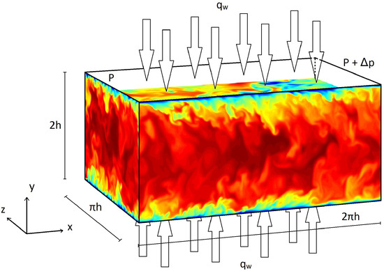
Figure 1.
Geometry and instantaneous representation of the temperature field.
As it was said above, the computational box was optimized in [25]. The dimensions of the box are , and in the streamwise, wall-normal, and spanwise directions, respectively. Coordinates in these directions are denoted by x, and z. The corresponding velocities are U, and W, or, using index notation, . This is also the case for vorticity, and helicity . Temperature is represented by T. However, the transformed temperature, (defined below), will be used during the entire paper. Uppercase letters denote instantaneous flow magnitudes. Using the Reynolds decomposition, one can obtain the averaged value, denoted by an overbar, and the fluctuating part, denoted by a lowercase letter, of the flow magnitudes, i.e., . The superscript + indicates normalization in wall units, using and , where is the mean shear stress and is the fluid density.
The behavior of turbulent flows is described by the Navier–Stokes equations, which are composed by the continuity and momentum equations,
and the energy equation,
where is the average of in time and in the three spatial directions, i.e., , where is the bulk velocity. In the energy equation, the transformed temperature, is used. Since the MBC is used, the temperature in the channel increases linearly in the streamwise direction and periodic conditions cannot be used for T. contains the nonperiodic part of the temperature, which makes periodic in the streamwise direction. Notice that the method described below is also useful for any other passive scalar, as it could be NOx concentration. It is also important to point out that for clarity, only the system with one energy equation will be explained here. However, as heat transfer is treated as a passive scalar, several different Prandtl numbers can be run simultaneously. In what follows and to facilitate the discussion, + superscripts will be omitted.
Using some algebra, which involves taking the rotational of Equations (1) and (2) twice, these equations can be written in velocity-vorticity form obtaining a fourth-order equation for V
and a second-order equation for
where and collect the nonlinear part of the Equations (4) and (5), and are given by
The main advantage of this system is that pressure is not present, simplifying the problem. Notice that one can easily recover velocities and vorticities from the continuity equation and the definition of ,
Taking derivatives,
and reorganizing the terms, we get
As the flow is periodic in both x and it is natural to use Fourier methods in these directions. The Fourier transform of any field is defined as
where the hat indicates the Fourier coefficient, and and are the wavenumbers in x and respectively. Equations (10) and (11) can be trivially solved as they become
Notice that this technique cannot be used for the -modes of U and Using the Navier–Stokes equations, one can write
and solve these equations instead. The pressure gradient in the spanwise direction is negligible. However, the pressure gradient in the streamwise component can be used to keep the flow mass constant. Using Fourier transforms, Equations (3)–(5) are transformed into Fourier space in x and z, obtaining three decoupled problems,
where is the Fourier transform of the energy equation nonlinear term.
Problem (14)–(16) is usually solved splitting in three parts, (wavenumbers are omitted)
where a and b are chosen in order to fulfill the homogeneous Neumann condition:
and
although, due to the symmetry of the problem, so only Equations (21), (22), (24) and (25) have to be solved. Notice that 3D PDE have been transformed into independent problems.
3. Numerical Method
3.1. CFD Techniques
As it is said above, Fourier method in x and z is the best option to solve this problem. This, in fact, decouples the problems (21)–(25) in a large amount of problems in y. The numerical technique used for y is thus critical to obtain an accurate and fast algorithm. This kind of problem had been addressed mostly by spectral methods [9,31]. A typical technique used in channels is Chebyshev polynomials [11,32]. This has also been applied to thermoconvective problems [33,34,35]. However, in this case, it is more efficient the use of Compact Finite Differences, CFD. The CFD method was introduced in a groundbreaking article by SK Lele in 1992 [36]. Lele’s idea was to use finite differences to solve problems presenting a range of spatial scales, generalizing some Padé schemes that had been used early [37,38]. Lele’s CFD main advantage is that maintaining the freedom in choosing the mesh points of typical finite difference methods (FD), offering very high precision, comparable to spectral methods. This is critical in turbulent problems, as one typically needs many more points close to the wall than in the outer regions of the flow.
Throughout this part of this work, the following notation is going to be used. Let be a real evaluated function. Supposing that u is differentiable enough, the first and second derivative of u at the point will be denoted by and . In the case of a derivative of grade n, we will use . Here, is a point belonging to a certain discretization of the interval , where a and b are finite and , . Without loss of generality, we will focus on schemes for the second derivative. FD schemes aim to compute an approximation of trough a linear combination of the values of the function close to . CFD, instead, relates a linear combination of the second derivatives with the values of the function. To explain the practical use of CFD schemes, we are going to work with one specific example, the scheme used in [29]. In that work, the authors used a stencil of seven points in the function and five in the second derivative. Let us assume that the following relation holds
for some unknowns coefficients, and . Without loss of generality, it is possible to assume that one of these coefficients is one, so from now on, . Defining , Taylor’s Theorem states that
and
The relations between the coefficients and are derived by matching the Taylor series coefficients. In this case, the formal truncation error of the approximation is tenth order. Translating this information into an algebraic equation leads to the system
Please note that this is the direct matrix coming from matching Taylor’s expansions. Usually, this matrix is ill-conditioned, so results can be very inaccurate. A typical procedure to overcome this problem consists of normalizing each row by its absolute value maximum.
As the mesh can be nonuniform, it is necessary to solve this system for each point in the mesh. When approaching the boundaries, no ghost points are used but the stencils are adapted, removing the points which lay outside the interval. This reduces the formal truncation error of the system. Once the coefficients for every point have been computed, we obtain two sparse matrices, one containing the coefficients, , and another one made by the coefficients, , such that
where the superscript denotes the transpose. Note that (28) can be used in both ways, to derive a function or to integrate it.
3.2. Time Discretization
To get good accuracy in reasonable computation times, a third-order Runge–Kutta method has been chosen, derived in [39]. For any problem with the form
where L is a linear operator and N is nonlinear, the equation is discretized as follows:
with for This method presents two problems. The first one is a problem of memory, due to the necessity of saving two nonlinear terms in steps two and three. The second problem is a possible loss of accuracy near the wall, due to the explicit computation of the linear operator in the right hand,
Both problems are solved in the algorithm, using a little bit of algebra. Suppose that (30) is solved, and is to be computed. Let us denote
then
and we can compute and store in a single buffer of memory the right hand side of (31) except the nonlinear term . This tactic can be also applied in the computation of but only in the cases where does not change. If the time step changes, the derivative of has to be computed explicitly. To avoid this loss of accuracy, it is a good idea to recompute the maximum every few steps, using the Courant–Friedichs–Lewy condition
The simulations made with this code ran with a CFL of showing remarkable stability.
Equations (30)–(32) are solved for , and using CFD. In what follows we will work with the energy equation, given that the linear operator is for and and for The operator L in Fourier space can be written as
Denoting by the right-hand side of (30)–(32), this system becomes
In Fourier space, one gets
Now using the two matrix described in the CFD section (28), and defining as the first constant of the previous equation,
we get
Defining a new matrix as
the final problem to solve is
Notice that this matrix is banded, which allows low-storage schemes and the use of very efficient LAPACK routines.
4. Parallelization Strategy
The most expensive part of the algorithm is the computation of the nonlinear terms , and . This is because it is necessary to compute these terms in physical space, due to the aliasing problem [31]. Notice that there are two global operations:
- Direct and inverse Fourier transforms in x and z, as the nonlinear term has to be computed in physical space.
- Integration-derivation in y.
As the data is distributed throughout the supercomputer, it is necessary to perform several all-to-all communications, which are critical and extremely demanding of the fast network of the supercomputer. The code demands a total of global communications per step, where is the total number of heat transfer problems studied.
The number of points of the problem, and thus memory, depend on the Reynolds number studied. Another constraint is the efficiency of the fast Fourier transforms (FFT), so typically numbers made up of powers of 2 and 3 are chosen to increase the velocity of the FFT. Assuming a mesh with points, generally is the largest one. It is then natural to start each substep of the Runge–Kutta scheme with the data set distributed in y–z planes. To avoid load imbalances, the number of nodes must be a divisor of the number of complex planes, which is after dealiasing. This number is also the maximum number of nodes that can be used. The maximum number of OpenMP processes at each node is where is the number of processors of the node.
The code to implement the algorithm described above, where Figure 2 can serve as roadmap, is as follows
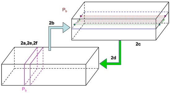
Figure 2.
Parallelization scheme of the code.
- Read data and configuration files: HDF5
- Runge–Kutta, data: , and in Fourier Space, distributed through the supercomputer with a shape.
- (a)
- Calculation of nonlinear terms (I). Time: 15% of total time
- .
- Compute statistical quantities of the flow if needed.
- Change shape from to
- Perform inverse transforms in z of and
- (b)
- Calculation on nonlinear terms (II). Time: 35% of total time
- Global transposes: Data is moved trough all the machine, from y–z planes into x-lines using MPI routines.
- (c)
- Calculation on nonlinear terms (III). Time:10% of total time
- Perform inverse transforms in x of and .
- Computes three technical buffers to compute later the nonlinear terms and . is computed here.
- Perform direct transforms in x of and
- (d)
- Calculation on nonlinear terms (IV). Time: 20% of total time
- Global transposes: Data is moved trough all the machine, from x-lines into y–z planes
- (e)
- Calculation on nonlinear terms (V). Time: 10% of total time
- Perform direct transforms in z of and
- Change shape from to
- (f)
- Solve viscous problem. This step requires 10% of total time.
- (g)
- Save data to disk if needed.
- (h)
- Move to the step 2a.
- End of program.
The code spends 90% of the time and almost all communication time computing the nonlinear term and only 10% to actually solve the equations. A large share of this 90% is used to do global communications. This is a critical step and requires an in-deep study of the supercomputer where the simulation is going to run.
Finally, notice that while global communications uses MPI routines, the granularity of the code makes the use of OpenMP routines for the Fourier transforms, derivatives, and the viscous step. This is an important advantage due to the foreseen evolution of supercomputation.
5. Conclusions
The main goal of this work is to develop a code to perform direct numerical simulations of distinctive wall-bounded thermal canonical flows. This code has run for roughly 50 CPU-M hours in several supercomputers, already producing several articles. FFT and CFD techniques have been described—in particular, how to use a nonequispaced grid for CFD. In addition, the combination of the Runge–Kutta time-stepper and the previous techniques have been explained. Finally, the parallelization scheme has been outlined. Its main advantage is the granularity of the data, allowing a large amount of small problems in each step that can be solved efficiently using OpenMP techniques.
The raw data that support the findings of this study are available from the corresponding author upon reasonable request. One point statistics can be downloaded from the web page of our group: http://personales.upv.es/serhocal/ (accessed on 24 March 2021).
Author Contributions
Conceptualization, F.Á.-Á.; Data curation, M.J.P.-Q.; Formal analysis, F.L.-R., F.Á.-Á. and S.H.; Funding acquisition, S.H.; Investigation, S.H.; Methodology, F.L.-R.; Resources, M.J.P.-Q.; Software, F.L.-R., M.J.P.-Q. and S.H.; Validation, F.Á.-Á.; Visualization, F.Á.-Á.; Writing—original draft, S.H.; Writing—review & editing, F.Á.-Á. All authors have read and agreed to the published version of the manuscript.
Funding
This work was supported by RTI2018-102256-B-I00 of MINECO/FEDER. The computations of the new simulations were made possible by several generous grants of computing time from the Barcelona Supercomputing Centre, references FI-2018-1-0037, FI-2018-2-0021, FI-2018-3-0032, FI-2019-1-0025, IM-2019-2-2016, AECT-2020-1-0024, AECT-2020-2-0005.
Institutional Review Board Statement
Not applicable.
Informed Consent Statement
Not applicable.
Data Availability Statement
Not applicable.
Acknowledgments
S.H. is deeply indebted and grateful to his students of the Master of Aerospace Engineering, Universitat Politècnica de València.
Conflicts of Interest
The authors declare no conflict of interest.
Abbreviations
The following abbreviations are used in this manuscript:
| CFD | Compact Finite Differences |
| DNS | Direct Numerical Simulation |
| FD | Finite Differences |
| FFT | Fast Fourier Transform |
| LES | Large Eddy Simulations |
| ODE | Ordinary differential equation |
| PDE | Partial differential equation |
| RANS | Reynolds Averaged Navier Stokes |
References
- Pope, S.B. Turbulent Flows; Cambridge University Press: Cambridge, UK, 2000. [Google Scholar]
- Margot, X.; Hoyas, S.; Fajardo, P.; Patouna, S. A moving mesh generation strategy for solving an injector internal flow problem. Math. Comput. Model. 2010, 52, 1143–1150. [Google Scholar] [CrossRef]
- Margot, X.; Hoyas, S.; Fajardo, P.; Patouna, S. CFD study of needle motion influence on the exit flowconditions of single-hole injectors. At. Sprays 2011, 21, 31–40. [Google Scholar] [CrossRef]
- Escarti-Guillem, M.; Hoyas, S.; García-Raffi, L. Rocket plume URANS simulation using OpenFOAM. Results Eng. 2019, 4, 100056. [Google Scholar] [CrossRef]
- Lluesma-Rodríguez, F.; González, T.; Hoyas, S. CFD simulation of a hyperloop capsule inside a closed environment. Results Eng. 2021, 9, 100196. [Google Scholar] [CrossRef]
- Kolmogorov, A.N. Local structure of turbulence in an incompressible fluid at very high Reynolds numbers. Dokl. Akad. Nauk. 1941, 30, 9–13. [Google Scholar] [CrossRef]
- Kolmogorov, A.N. Dissipation of energy in isotropic turbulence. Dokl. Akad. Nauk. 1941, 32, 19–21. [Google Scholar]
- Samie, M.; Marusic, I.; Hutchins, N.; Fu, M.; Fan, Y.; Hultmark, M.; Smits, A. Fully resolved measurements of turbulent boundary layer flows up to Reτ = 20000. J. Fluid Mech. 2018, 851, 391–415. [Google Scholar] [CrossRef]
- Kim, J.; Moin, P.; Moser, R. Turbulence statistics in fully developed channels flows at low Reynolds numbers. J. Fluid Mech. 1987, 177, 133–166. [Google Scholar] [CrossRef]
- Spalart, P. Direct simulation of a turbulent boundary layer up to Rθ = 1410. J. Fluid Mech. 1988, 187, 61–98. [Google Scholar] [CrossRef]
- Moser, R.; Kim, J.; Mansour, N. Direct numerical simulation of turbulent channel flow up to Reτ = 590. Phys. Fluids 1999, 11, 943–945. [Google Scholar] [CrossRef]
- Hoyas, S.; Jiménez, J. Scaling of the velocity fluctuations in turbulent channels up to Reτ = 2003. Phys. Fluids 2006, 18, 011702. [Google Scholar] [CrossRef]
- Hoyas, S.; Jiménez, J. Reynolds number effects on the Reynolds-stress budgets in turbulent channels. Phys. Fluids 2008, 20, 101511. [Google Scholar] [CrossRef]
- Simens, M.P.; Jimenez, J.; Hoyas, S.; Mizuno, Y. A high-resolution code for turbulent boundary layers. J. Comput. Phys. 2009, 228, 4218–4231. [Google Scholar] [CrossRef]
- Lee, M.; Moser, R. Direct numerical simulation of turbulent channel flow up to Reτ ≈ 5200. J. Fluid Mech. 2015, 774, 395–415. [Google Scholar] [CrossRef]
- Lozano-Durán, A.; Jiménez, J. Effect of the computational domain on direct simulations of turbulent channels up to Reτ = 4200. Phys. Fluids 2014, 26, 011702. [Google Scholar] [CrossRef]
- Bernardini, M.; Pirozzoli, S.; Orlandi, P. Velocity statistics in turbulent channel flow up to Reτ = 4000. J. Fluid Mech. 2014, 758, 327–343. [Google Scholar]
- Avsarkisov, V.; Hoyas, S.; Oberlack, M.; García-Galache, J. Turbulent plane Couette flow at moderately high Reynolds number. J. Fluid Mech. 2014, 751, R1. [Google Scholar] [CrossRef]
- Kraheberger, S.; Hoyas, S.; Oberlack, M. DNS of a turbulent Couette flow at constant wall transpiration up to Reτ = 1000. J. Fluid Mech. 2018, 835, 421–443. [Google Scholar] [CrossRef]
- Kim, J.; Moin, P. Transport of Passive Scalars in a Turbulent Channel Flow; NASA: Ames Research Center: Moffett Field, CA, USA, 1987; Volume 1, pp. 1–14. [Google Scholar]
- Lyons, S.; Hanratty, T.; McLaughlin, J. Direct numerical simulation of passive heat transfer in a turbulent channel flow. Int. J. Heat Mass Transf. 1991, 34, 1149–1161. [Google Scholar] [CrossRef]
- Kasagi, N.; Tomita, Y.; Kuroda, A. Direct Numerical Simulation of Passive Scalar Field in a Turbulent Channel Flow. J. Heat Transf. 1992, 114, 598–606. [Google Scholar] [CrossRef]
- Piller, M. Direct numerical simulation of turbulent forced convection in a pipe. Int. J. Numer. Methods Fluids 2005, 49, 583–602. [Google Scholar] [CrossRef]
- Yano, T.; Kasagi, N. Direct numerical simulation of turbulent heat transport at high Prandtl numbers. JSME Int. J. Ser. B Fluids Therm. Eng. 1999, 42, 284–292. [Google Scholar] [CrossRef]
- Lluesma-Rodríguez, F.; Hoyas, S.; Peréz-Quiles, M. Influence of the computational domain on DNS of turbulent heat transfer up to Reτ = 2000 for Pr = 0.71. Int. J. Heat Mass Transf. 2018, 122, 983–992. [Google Scholar] [CrossRef]
- Alcántara-Ávila, F.; Hoyas, S.; Pérez-Quiles, M. DNS of thermal channel flow up to Reτ = 2000 for medium to low Prandtl numbers. Int. J. Heat Mass Transf. 2018, 127, 349–361. [Google Scholar] [CrossRef]
- Alcántara-Ávila, F.; Barberá, G.; Hoyas, S. Evidences of persisting thermal structures in Couette flows. Int. J. Heat Fluid Flow 2019, 76, 287–295. [Google Scholar] [CrossRef]
- Alcántara-Ávila, F.; Hoyas, S. Direct Numerical Simulation of thermal channel flow for medium–high Prandtl numbers up to Reτ = 2000. Int. J. Heat Mass Transf. 2021. submitted. [Google Scholar]
- Alcántara-Ávila, F.; Hoyas, S.; Pérez-Quiles, M. Direct Numerical Simulation of thermal channel fow for Reτ = 5000 and Pr = 0.71. Accept. J. Fluid Mech. 2021. [Google Scholar] [CrossRef]
- Gandía Barberá, S.; Alcántara-Ávila, F.; Hoyas, S.; Avsarkisov, V. Stratification effect on extreme-scale rolls in plane Couette flows. Phys. Rev. E 2021, 6, 034605. [Google Scholar] [CrossRef]
- Canuto, C.; Hussaini, M.Y.; Quarteroni, A.M.; Thomas, A., Jr. Spectral Methods in Fluid Dynamics; Springer Science & Business Media: Berlin/Heidelberg, Germany, 2012. [Google Scholar]
- Del Alamo, J.; Jiménez, J.; Zandonade, P.; Moser, R. Scaling of the energy spectra of turbulent channels. J. Fluid Mech. 2004, 500, 135–144. [Google Scholar] [CrossRef]
- Hoyas, S.; Herrero, H.; Mancho, A. Thermocapillar and thermogravitatory waves in a convection problem. Theor. Comput. Fluid Dyn. 2004, 18, 309–321. [Google Scholar] [CrossRef]
- Hoyas, S.; Gil, A.; Fajardo, P.; Pérez-Quiles, M. Codimension-three bifurcations in a Bénard-Marangoni problem. Phys. Rev. E Stat. Nonlinear Soft Matter Phys. 2013, 88, 015001. [Google Scholar] [CrossRef] [PubMed]
- Hoyas, S.; Fajardo, P.; Pérez-Quiles, M. Influence of geometrical parameters on the linear stability of a Bénard-Marangoni problem. Phys. Rev. E 2016, 93, 043105. [Google Scholar] [CrossRef] [PubMed]
- Lele, S.K. Compact finite difference schemes with spectral-like resolution. J. Comput. Phys. 1992, 103, 16–42. [Google Scholar] [CrossRef]
- Orszag, S.A.; Israeli, M. Numerical Simulation of Viscous Incompressible Flows. Annu. Rev. Fluid Mech. 1974, 6, 281–318. [Google Scholar] [CrossRef]
- Rubin, S.; Khosla, P. Polynomial interpolation methods for viscous flow calculations. J. Comput. Phys. 1977, 24, 217–244. [Google Scholar] [CrossRef]
- Spalart, P.R.; Moser, R.D.; Rogers, M.M. Spectral methods for the Navier-Stokes equations with one infinite and two periodic directions. J. Comput. Phys. 1991, 96, 297–324. [Google Scholar] [CrossRef]
Publisher’s Note: MDPI stays neutral with regard to jurisdictional claims in published maps and institutional affiliations. |
© 2021 by the authors. Licensee MDPI, Basel, Switzerland. This article is an open access article distributed under the terms and conditions of the Creative Commons Attribution (CC BY) license (https://creativecommons.org/licenses/by/4.0/).