
Normalized Information Criteria and Model Selection in the Presence of Missing Data

Department of Industrial Engineering and Management, Ben-Gurion University of the Negev, P.O. Box 653, Beer-Sheva 84105, Israel
*
Author to whom correspondence should be addressed.
Mathematics 2021, 9(19), 2474; https://doi.org/10.3390/math9192474
Submission received: 1 August 2021
/
Revised: 6 September 2021
/
Accepted: 27 September 2021
/
Published: 3 October 2021
(This article belongs to the Special Issue Methods and Applications of Statistics in the Social and Health Sciences)
Abstract
:Information criteria such as the Akaike information criterion (AIC) and Bayesian information criterion (BIC) are commonly used for model selection. However, the current theory does not support unconventional data, so naive use of these criteria is not suitable for data with missing values. Imputation, at the core of most alternative methods, is both distorted as well as computationally demanding. We propose a new approach that enables the use of classic well-known information criteria for model selection when there are missing data. We adapt the current theory of information criteria through normalization, accounting for the different sample sizes used for each candidate model (focusing on AIC and BIC). Interestingly, when the sample sizes are different, our theoretical analysis finds that is the proper correction for that we need to optimize (where is the sample size available to the model) while is the correction of BIC. Furthermore, we find that the computational complexity of normalized information criteria methods is exponentially better than that of imputation methods. In a series of simulation studies, we find that normalized-AIC and normalized-BIC outperform previous methods (i.e., normalized-AIC is more efficient, and normalized BIC includes only important variables, although it tends to exclude some of them in cases of large correlation). We propose three additional methods aimed at increasing the statistical efficiency of normalized-AIC: post-selection imputation, Akaike sub-model averaging, and minimum-variance averaging. The latter succeeds in increasing efficiency further.
1. Introduction
In statistical research and data mining, methods for selecting the “best” model associated with the observed data are of great importance. This is especially crucial in areas such as healthcare and medical research, where the models themselves are very important (and so merely minimizing the generalization error directly, via cross-validation and non-parametric methods, will not suffice). Model selection takes a major role in regression analysis that searches for a set of variables that are “important", to compose a model that best explains some given data. In recent decades, a variety of methods have been developed for selecting models when the data are completely observed, in particular methods based on information criteria [1,2].
Information criteria are perhaps the most common tools used for model selection, through the process of comparing a quantitative score for each model and choosing the model with the best score. The information criterion score is a trade-off between goodness-of-fit and the complexity of the model: specifically , where is the maximized likelihood of the candidate model, and the penalty term takes into consideration the complexity of the sub-model. Perhaps the most common information criterion today is the Akaike information criterion (AIC), first introduced by [3,4], where the AIC penalty is simply , twice the number of parameters in the model. The idea of this information criterion was derived from the Kullback–Leibler (KL) divergence, a quantitative measure of directed distance between two models. AIC estimates how much information is lost when approximating the true unknown model, which actually generated the observed data, with the estimated model.
Another common information criterion is the Bayesian information criterion (BIC) presented by [5], which has penalty , where n is the number of observations. BIC was derived from Bayesian theory, based on the Bayes factor approach. It is an approximation to the Bayes factor, which selects the model with the greatest posterior probability. Unlike the AIC, it is asymptotically consistent—it will select the true model if it is among the candidate models considered—but it is inefficient for prediction (in contrast to AIC, which is asymptotically efficient for prediction). This criterion is used when trying to understand which of the variables explain the data, and find the model most likely to be true [1,6].
A problem with both of these methods is that they are not suitable where the data contain missing values. Model selection in the presence of missing data is a major challenge, even when the data are missing completely at random, MCAR, (here we use Rubin’s taxonomy for missingness [7,8,9]; cf. the recent and more comprehensive taxonomy by [10]).
In particular, suppose we have n independent observations, containing some missing values. Consider that we have a set of candidate models, , to choose from, in order to explain the observations. It might happen that each candidate model, , is based on a different sample size, . Figure 1 shows a setting of a design matrix in a regression model, where the various possible models do not have the same sample size; thus, implementing model selection using conventional information criteria is inappropriate.
Obviously, missing data are a problem for nearly all statistical applications, not just for model selection. Various methods have been developed to deal with this problem, most of which involve manipulating the data into a complete dataset, so a standard analysis can be performed. The common approaches for dealing with missing data ranges from complete cases analysis (which simply deletes all observations with one or more missing values, leaving a complete dataset so that a standard analysis can be performed) to single imputation and multiple imputation, which consists of three stages—imputation, analysis, and combination—all of which are required to properly account for the uncertainty of imputation [8,11]. Somewhat naturally, early work addressing missing data in the context of model selection took this approach and tried to adapt it; however, it is challenging to combine the results of variable selection (the last stage) across all imputed datasets in a principled framework, and there are a variety of articles on this issue [12,13,14,15,16,17].
Another strategy, presented by [12], is to combine multiple imputation and variable selection in a Bayesian framework. The authors of that study showed two methods for linear regression models with missing data in the covariates. The first method, impute then select (ITS), starts with generating different imputed datasets, then applies Bayesian variable selection methods for each imputed dataset, and uses Rubin’s rule to combine the results. The second method is simultaneously impute and select, which embeds the steps of imputation and variable selection in a single, combined Gibbs sampling process. The first method is easier to implement in standard software and enables flexible imputation and separate analysis, but the study’s results indicated that the second method slightly outperformed the first.
One more variable selection strategy is to combine resampling techniques with imputation, as presented by [18]. They developed the procedure of bootstrap imputation and stability selection, which generates bootstrap samples and conducts single imputation on each bootstrap dataset. It then obtains the randomized lasso estimate for each dataset, and the final variable selection is conducted by stability selection. The authors of [19] developed the similar method, multiple imputation random lasso, with the main difference being that their method first performs imputation, and only then generates bootstrap samples. Both sets of results showed that these approaches are suitable for high-dimensional problems. This approach, using imputation or expectation–maximization (and EM-like) to replace missing data, is present also in [20,21,22,23], cf. [24,25,26].
In this work we present a different approach, based on first principles of information criteria [3,4,5]. We propose to apply the information criteria to a candidate model by using all of its full observations, and then normalize, in some form, the information criteria according to sample size. In this way, the different models can be compared by the information criterion score per observation. Consider again the example in Figure 1, in order to calculate the information criterion of a model containing variables and , we will use only observations 5, 6, 7, and 10, and then normalize it to the number of observations, , to obtain the normalized information criterion. By contrast, in models containing and , we will use observations 7, 9, and 10 to calculate the information criterion and then normalize it to .
Here, we focus on two methods for model selection in the presence of missing data, which are based on the theory of existing AIC and BIC methods, and introduce normalized AIC and normalized BIC. The advantage of the new methods is the use of more observations than in “complete cases”, on the one hand, while avoiding unnecessary variance due to imputation, on the other (as well as savings in computational complexity compared to imputation methods).
The rest of this paper is organized as follows. In Section 2, we present the theory of normalized AIC and normalized BIC, which adapts current theory to cases where the data are missing. In Section 3, we discuss the computational efficiency [27] of the normalized information criteria, compared to imputation-based methods, as well as their statistical efficiency, and present three additional methods that extend the normalized AIC method from Section 2.1, in order to increase its statistical efficiency. Simulation results are provided in Section 4. We conclude this article in Section 5.
2. Normalized Information Criteria
Our theory of normalized AIC and normalized BIC relies on the traditional theory of AIC and BIC with changes due to relaxing the assumption that all candidate models have the same sample size; the new criteria makes no such assumption.
Suppose we have data that are independent and identically distributed i.i.d., drawn from some probability distribution with the unknown density , and we have a set of candidate models, , where each model is a family of probability densities, , depending on a parameter vector, . Where is the parameter space of model with dimension .
In the context of this paper, the data contains missing values. Each model is based on the observations that do not contain missing values, so each model can have different sample size , which is indicated by the subscript . The likelihood of the data, given the jth model based on observations is , and the maximum likelihood estimator of , based on data, is
2.1. Normalized AIC
The AIC is equal to , where k is the number of parameters in the model. Akaike recognized the properties of as a mean unbiased estimate of the expected relative KL distance between a candidate model and the “true” model, on data that are previously unseen; however, since the multiplicative factor shared by the AIC scores of all models do not affect their selection, it was disregarded, and subsequent research focused on the AIC score itself. We assume, on the other hand, that each candidate model, , is based on a different sample size, . Therefore, sample size n is no longer constant for all candidate models, and cannot be ignored.
The AIC is an estimation of the KL divergence for selecting the model that minimizes the information lost when candidate model, , is used to approximate the reality, f,
where is an unknown constant, equal for all candidate models, and the second term, the relative KL information, is the expectation with respect to the probability density, f. Note that the true model f is not necessarily in any of the candidate models. For all candidate models, we calculate the negative expected relative distance and select the model with the smallest value, i.e., the “closest” to
where x is a conceptual future random sample from distribution f, that play as “validation” set, to estimate , and assume to be independent sample from data . The expectations and are the expectation with respect to the true model, , over the random samples x and , respectively. If multiplied by 2 and it will produce , the AIC score for the candidate model .
Thus, the final criterion obtained for model is
The best model chosen by this method would be the one that minimizes the criterion. More detailed derivation of the AIC appears in Appendix A.
2.2. Normalized BIC
The BIC is , where k is the number of parameters in the model, and n is the number of observations. The BIC is a Bayesian method for selecting the model which maximizes the a posteriori probability of the model given the data. For all candidate models, , we calculate the posterior probability and select the model with the greatest value. According to Bayes’ theorem the posterior probability of model , given data comprised of observations, is
where is the prior probability of model , is the unconditional likelihood of the data comprised of observations, is the prior density of given model j, and is the marginal probability of the data for model j.
In case all prior probabilities are equal, i.e., and for all j, the critical quantity to be approximated is , because all other expressions in (1) are the same for all models. Thus, by maximizing this term the posterior probability will be maximized as well. In this standard case, BIC is obtained as
The best model chosen by the method would be the one that minimizes the criterion (i.e., maximizes the posterior probability). For a more detailed derivation of BIC see Appendix B. Similarly, in the case of different sample sizes, a “naive” BIC score can be calculated
however, now the denominator in (1) cannot be ignored. To maximize the posterior probability we need to maximize the quantity
We develop the log denominator of expression (3) as follows:
Assume , using the law of large numbers yield
and the log unconditional likelihood converges to
When comparing two models, we need to check whether
which is equivalent to
and from (2)–(4)
Instead of comparing each pair of models, it is possible to calculate the result for each model, , by comparing to the fixed model which consists of an intercept only, . Since uses all observations, the candidate models maximal sample size is that of the constant model, , we find that in case , the above is
and in case , the above is
Although the value of h is unknown, we can estimate it (The scalar parameter h is known as the entropy of the distribution g. Estimation of a scalar is generally much simpler than estimation of a distribution, and thus estimating h is easier compared to estimating g. However, here we do not even require estimating h and thus we do not discuss it further; this is left for future developments). Furthermore, as a simple substitute we can optimize the left-hand side, and select the model with the best ratio.
The final normalized BIC is calculated as follows for each model, : in the case , the score will be ; otherwise, and the score will be . The best model will be the one with the lowest score.
3. Statistical Efficiency and Computational Efficiency
The methods presented in Section 2 introduce a benefit in terms of statistical efficiency. First, they are statistically efficient in the sense that they uses all cases completely observed for a candidate model. Unlike complete-cases analysis, where each candidate model uses only the cases completely observed of the data, the new proposed methods use a larger fraction of the original data so the model selection procedure is more efficient. Second, the new methods avoid the addition of “noise” and unnecessary variance due to imputation.
In addition to being advantageous in terms of statistical efficiency, the normalized information criteria are also advantageous in terms of computational efficiency (see also [27]). They do not require a procedure for filling in missing values as in imputation method, and moreover the model selection procedure processes less data for each candidate model.
3.1. Computational Efficiency
In this section, we compare the computational efficiency of model selection of normalized-information-criterion methods and the computational efficiency of single-imputation methods; we find that under a MCAR assumption, imputation, which considers a complete dataset after filling in the missing data, can be exponentially less efficient.
Consider the following crude toy example of “all subset regression” (exhaustively comparing all possible models in the candidate set) and examining how much data are being processed by the model-selection procedures:
Assume a global model that contains d variables and n observations, and the goal is to choose the best model among a set of candidate models, . This set of models is the subset of the global model with all possible combination of the variables, so the total number of models in the set of candidates is . The number of models in that contain exactly j variables, where , is . Each model , containing j variables can be represented by an rectangle data matrix. These are the data each model m receives, so in case missing values do not occur, the “data size” for model m with j variables is exactly the multiplication between the number of variables and the number of observation: .
Under MCAR, each entry is missing with probability p, independently for all entries. The probability of single observation (i.e., row) with j variables to be completely observed is , and the number of observations completely observed out of n possible observations is binomially distributed with parameter n and probability ; therefore, the expected value of the number of completely observed observations is
The expected “data size” of model m with j variables in case of MCAR is the expected number of complete observations multiplied by the number of variables:
In order to obtain the computational efficiency of both methods, we calculate the “size of the data” each method processes during the model selection procedure; i.e., the “data size” each model m receives and summing it up over all candidate models under consideration in the procedure. This size is a function of the number of observations in the global model, n, the number of variables in the global model, d, and the missingness probability per entry of the data, p.
In order to calculate the computational complexity of model selection with single imputation we set aside the fill-in procedure, and only calculates as if the missingness probability is 0 (due to the completion of the missing values). Thus, each model has the same number of observed data n exactly:
As mentioned above, the number of models in that contain j variables are , and the data size is the multiplication . Using Newton’s binomial formula, we obtain
To find the computational complexity of the normalized-information-criterion methods, a similar calculation is made, but this time each value is observed with probability
Further, is the number of models in that contain j variables, and the data size is the multiplication mention before . Using Newton’s binomial formula (after integration with respect to p), we obtain
Calculating the computational efficiency ratio between the single imputation methods (5) and normalized information criterion methods (6) yields
Hence, the improvement in computational efficiency increases exponentially as the number of variables increases; i.e., using normalized information criteria significantly reduces computational complexity, compared to single imputation.
A similar simple calculation for other scenarios, such as forward-selection, would yield results that might be less overwhelming but substantial nonetheless. Indeed, for forward selection the ratio in computational efficiency increases quadratically (though this is more nuanced, and in addition to it depends also on , the number of variables in the chosen model).
3.2. Increasing the Statistical Efficiency
The new methods are statistically efficiencies since they uses more observations then complete cases, and they do not add additional noise as imputation methods.
However, they do not use all available information for each model, as opposed to imputation mathods that uses all observed data. For example, suppose that, in a regression model with missing values in the design matrix, the model selected by normalized AIC contains the variables and . Figure 2a illustrates the data available for the selected model, completely ignoring the other variables. In calculating the normalized AIC, only observations 3, 6, 9, and 10 are used, while the rest of the available values, marked in white, are not used.
To address the inefficiency issue of the preliminary normalized AIC procedure discussed in Section 2.1, we propose three additional methods that extend the normalized AIC, called post-selection imputation, Akaike sub-model averaging, and minimum variance averaging. These methods use all of the observed information relevant to the model chosen by the method normalized AIC in order to increase its efficiency. All methods use only the data from the selected model and completely ignore variables that are not part of the chosen model.
3.2.1. Post-Selection Imputation
Imputation is performed only after the removal of “unwanted” columns, identified using our selection procedure. For instance, in Figure 2a, the method will first fill in the missing values, marked in black, and only then estimate the parameters.
3.2.2. Akaike Sub-Model Averaging
After identifying the “best” model, it is possible to make use of its nested models, which add additional data. For example, in Figure 2a, the model has three sub-models: first, a model containing only variable ; second, a model containing only variable ; and third, a model containing variables and .
This procedure (as well as the procedure in Section 3.2.3) will include all observations relevant to the sub-model, based on the values that do exist in that observation. As an illustration, Figure 2 shows how the observations are associated with their respective models. In Figure 2b, all observations which contain values of variable will be associated with the first model, which contains only variable . Those observations (3, 5, 6, 7, 9, and 10) are highlighted. Similarly, Figure 2c highlights the observations (2, 3, 4, 6, 8, 9, and 10) associated with the second model, which contains variable . Finally, Figure 2d highlights the observations (3, 6, 9, and 10) belonging to the third model—the full model. Note that the best (full) model has the minimal sample size.
We will use model averaging by determining their associated weights, akin to Akaike weights [2,28,29]. We take a similar approach as we did in Section 2.2, by finding the “posterior” distribution of each sub-model, and approximate the log posterior odds from the best model. Further, we assume that the priori probabilities are the same, but the denominator probabilities are not, and therefore we will not ignore it.
The posterior distribution of model j is
where is the prior probability of model , is the unconditional likelihood of the data comprised of observations and is the marginal probability of the data for model j.
Akaike recognize the quantity as the “likelihood” of the model determined by the method of maximum likelihood [30,31,32], so
We develop the denominator of expression (7) exactly the same as in Equation (4), and obtain
In case all prior probabilities are equal, and from (7)–(9), we obtain the quantity
In order to use (10) as weights we can solve for the h which yields ; however, there is a simpler albeit cruder approach:
Let be the model chosen by the normalized AIC procedure, so it minimize the score
where t is the number of existing sub-models of in the original dataset.
Similar to Section 2.2 let us define the relative difference
where the second case yields the same relative difference as the original Akaike weights. The sub-model weights, , obtain by finding the relative difference for each model, , and substitute it in the following equation
The proposed weights have similar characteristics to the original Akaike weights. We strive to minimize the proposed relative difference, so “closer” models (with lower AIC) have a higher weight and vice versa. In addition, the relative difference is always non-negative, , and specifically zero for the best model. Another feature that corresponds to missing data is to provide greater weights to models with larger sample sizes, which increases the statistical power.
The weight has the heuristic interpretation as the probability that is the best model, given the data and the set of sub-models. The final prediction estimation obtain by linear combination of all sub-models estimates with their associate weights
This is further examined below via simulations.
3.2.3. Minimal Variance Sub-Model Averaging
The method presented in Section 3.2.2 might ignore the correlation that exists between the different models. We propose another method for sub-model averaging that takes into account the correlation between the models. The motivation of this method is the same as the previous method—making use of the nested models within the “best” model, which utilizes additional data. As mention before, the final prediction estimation obtains by a linear combination of all sub-models estimates with their associate weights, as in (11).
The variance of is
where is the weights vector, is the estimates generalization error (mean-squared error; MSE) covariance matrix of the models, and t is the number of existing sub-models in the original selected dataset by the normalized AIC.
We will use model averaging by determining their appropriate weights, proportional to the inverse generalization MSE covariance matrix of the models. The weights vector are obtained by minimizing the variance using Lagrangian multipliers with the constraint yielding
where U is a vector of 1’s. This weights are the optimal minimum variance thus minimize the MSE.
The procedure will assign large weight to models with small variance, and small weight to models with large variance, taking into account the correlation between the models.
In order to obtain the MSE covariance matrix we use the well-known bootstrap method, introduce by [33] and extensively described in [34]. Our procedure start by resampling observations independently with replacement from the selected dataset, until sample size is equal to that for the original data set, n. These samples will serve as bootstrap train dataset. The probability that an observation does not appear in a bootstrap sample is as , so the expected number of observation not chosen is and these observations will serve as a validation dataset.
Each bootstrap sample i (), estimates the vector and each component j () is calculated as
where i is the bootstrap sample index and j is the model index. This process repeated B times, resulting in B bootstrap samples and B estimators, which combine to the estimate MSE matrix. These matrix is then used to compute the variance-covariance matrix of the models, .
4. Simulation Studies
In order to investigate the statistical properties of the normalized information criteria for modeling selection with missing data, we performed a series of simulations using R.
4.1. Design
The data were simulated in the form of a linear regression model , where is the vector of dependent variables, is the design matrix, and is the noise vector, whose entries are i.i.d. and normally distributed with mean zero and variance 2.5, i.e., . The design matrix is composed of explanatory variables, which were generated from a multivariate normal distribution with symmetric correlation matrix with equal off-diagonal elements, denoted as ; where three different off-diagonal elements were considered: , , and . The coefficients were set to be , , , , and , so the “real” model comprises the variables , , , and . The response vector, , was obtained by the aforementioned linear regression. 400 observations were generated, and for the AIC methods outlined in Section 2.1 and Section 3.2, an additional 200 observations were treated as “test” data for model validation, with the remaining observations being “training” data, used to fit the models.
We created missing data by omitting some of the values from the design matrix (the training design matrix for AIC methods). We explored the MCAR missingness mechanism with two different missingness probabilities, and per observation, so that there were approximately and complete cases, respectively. With this simulation configuration there are six different design factors for all combinations of different effect of the correlation parameters () and missingness probabilities (p). For each of those six simulation configurations, 100 different datasets with missing values were simulated. The candidate models, , are all-subset regressions, so there are possible models.
4.2. Comparing Model Selection Results between AIC Methods
The normalized AIC method calculates for each candidate model, , the normalized AIC score, , according to the number of observations that the model was based on, . The model with the minimal score is selected. The methods that extend the normalized AIC are based on the results of normalized AIC. These methods were compared to complete case, single imputation, and multiple-imputation methods. Single imputation and multiple imputation was performed using MICE package [35], with one and five imputations respectively. For all these three methods, the regular AIC score was calculated for all possible models.
Each method was applied to each of the 100 datasets, where for each dataset the generalization error (MSE) of the chosen model was calculated over a test-set as . Then, the MSE was averaged over 100 simulated datasets. Overall, for each method, a total of six average MSE for each of the different configurations was calculated for comparison purposes. To test the statistical significance of the difference between the competing average scores, a two-tailed paired t-test was performed, with significance level 0.05.
4.2.1. Normalized AIC
Figure 3 presents the comparisons between the normalized AIC method and the other three methods. Each plot shows the MSE result averaged over 100 simulation datasets for the six different designs. Full circle markings indicate that the result is significant according to paired t-test, and empty markings indicate otherwise.
Figure 3a shows the comparison of normalized AIC to complete cases, and in Figure 3b the comparison of normalized AIC to single imputation is shown. It can be seen that for both comparisons, and for all the different configurations, the normalized AIC method yields better results, and is statistically more efficient. For almost all the comparisons made, the results are significant (except in Figure 3b, at and ).
On the other hand, in Figure 3c, which compares normalized AIC to multiple imputation, there is no method that achieves better results for all configurations and all results are not significant; therefore, the results are inconclusive and both methods are fairly on par. As expected, all methods yield better results for small missingness probabilities and lower correlations.
4.2.2. Extensions of Normalized AIC
In this section, we examine the methods that build on the normalized AIC approach. Post-selection imputation, Akaike sub-model averaging, and minimum variance averaging methods make use of only the variables chosen by the normalized-AIC method. For the chosen model, each method re-estimates the predictions. In post-selection imputation, multiple imputation is performed with the MICE package, and five imputations are made. In minimum variance averaging, bootstrap samples are made. Figure 4, Figure 5 and Figure 6 compares the extension methods to normalized AIC, multiple imputation and to each other, respectively. They summarize the average generalization MSE score for all six different designs. Here, too, full circles indicate statistically significantly differences.
Figure 4 compares normalized AIC and the methods extending it and examines whether the methods succeed in improving its statistical efficiency. Figure 4a, comparing post-selection imputation to the normalized AIC method, shows that post-selection imputation yields better results for all the different designs, significantly for higher missingness probabilities and higher correlations. Further, Figure 4b,c, compared to the Akaike sub-model averaging and minimum variance averaging to normalized AIC, respectively, shows that both extending methods yield better results for all six configurations significantly.
Figure 5 compares multiple imputation and the three extensions of normalized AIC methods: post-selection imputation (in Figure 5a), Akaike sub-model averaging (in Figure 5b), and minimum variance averaging (in Figure 5c).
It can be seen that all of the three extensions methods achieved lower MSE than multiple imputation, for all the different configurations. Post-selection imputation yields significant results for cases with and , and Akaike sub-model averaging yields significant results for all cases, except at and . Minimum variance averaging is significantly statistically more efficient for all six configurations.
Figure 6 compares the three methods extending the normalized AIC to each other.
Figure 6a, comparing Akaike sub-model averaging to post-selection imputation, shows that Akaike sub-model averaging yields better results for all the different configurations, significantly only at and and at and . Figure 6b, comparing minimum variance averaging to post-selection imputation, and Figure 6c, comparing minimum variance averaging to Akaike sub-model averaging, shows that minimum variance averaging succeed in minimized the MSE for both comparisons and all different configurations, significantly (except in Figure 6c, at and ).
Detailed numerical results for each method are provided in Appendix C.
4.3. Comparing Model Selection Results between BIC Methods
The normalized BIC method calculated for each candidate model, , the normalized BIC score according to the number of observations that the model was based on, . The score is if the sample size of model j is not completely observed (), and otherwise, where model 0 is the constant model. The model with the minimum score will be selected. Similar to the AIC method, the normalized BIC was compared to complete case, single imputation, and multiple imputation methods. For all these three methods, the regular BIC score was calculated.
In addition, we compared normalized BIC to an additional fourth method. We implemented a variation of the ITS method described in Section 1, which consists of three similar steps but uses different algorithms than those described in the original method in [12]. The first step is to perform multiple imputation, which is achieved using the MICE package, with imputed datasets. In the second step, a Bayesian variable selection algorithm is implemented for each dataset, l, separately, where . We implemented this using the BMS package [36]. Then, we calculated the posterior inclusion probability for each variable:
. In the third and final step, we combined the results using Rubin’s rules [7] to obtain the average marginal posterior probability of across L multiple imputation datasets defined as . The final variable selection is determined by whether exceeds the threshold of 0.5.
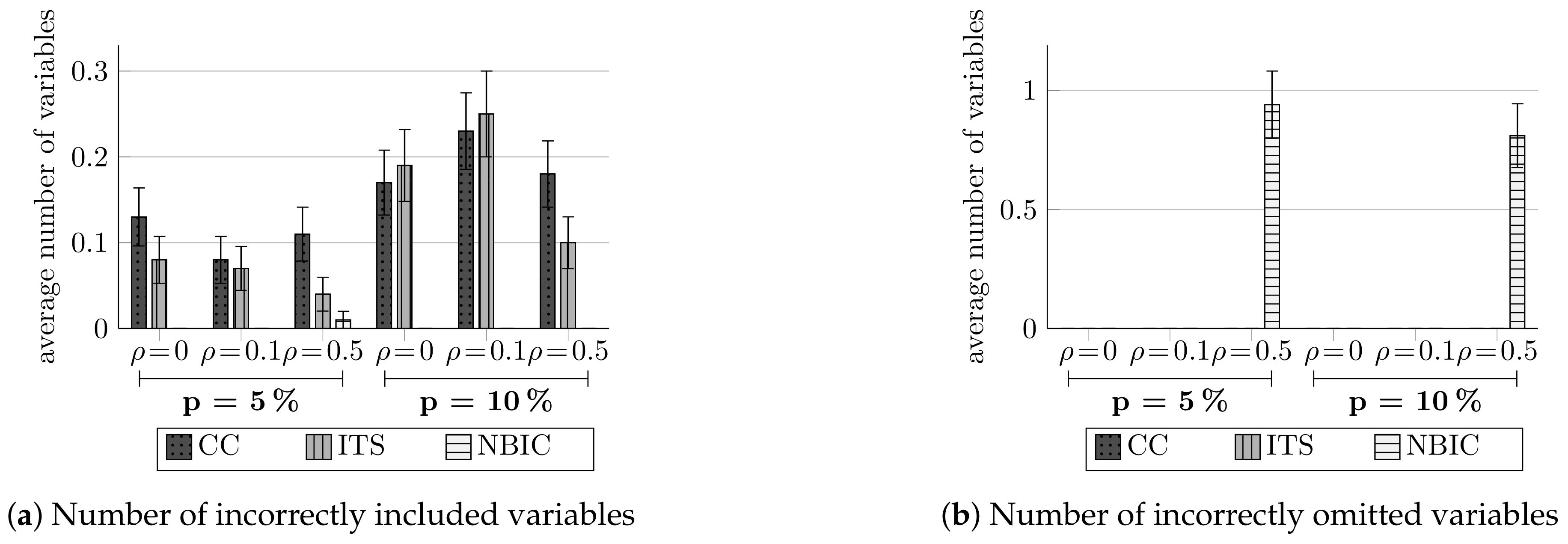
BIC methods were tested similarly to the AIC methods, only here, for each dataset the scores “incorrectly omitted” and “incorrectly included” were calculated for the chosen model and averaged over 100 simulated datasets. “Incorrectly omitted” is the number of important variables that were not selected in the chosen model (i.e., the number of variables from the important set, , , , and , not selected); and “incorrectly included” is the number of unimportant variables selected in the chosen model (i.e., the number of variables from the unimportant set, , , , , , and that were selected).
In Figure 7, we compared the normalized BIC method to complete case and ITS methods. Figure 7a provides the “incorrectly included” score for each different configuration and method. The results show that, while the other methods tend to include variables that are not important to the chosen model, the method we developed, normalized BIC, included only variables that were important. The results presented in Figure 7b summarize the “incorrectly omitted” score. It can be seen that all methods do not tend to exclude important variables, although when the correlation is large the normalized BIC method does tend to omit some.
The results of the single and multiple imputation methods were inferior to the other methods, so we do not present them here. Detailed numerical results for each method are provided in Appendix D.
5. Discussion
In this paper, we presented a new perspective on popular information criteria, specifically AIC and BIC, and developed a theory that adapts them to address data containing missing values. The traditional information criteria are not applicable in cases where data are missing, as they are based on the assumption that all models have the same constant sample size. The methods presented here address this issue by making slight modifications to the existing theory, required due to this non-assumption, and using the different sample sizes for each model to normalize its score. Thus, the score of each models is per-observation, which makes them comparable for model selection.
The methods we have introduced are intuitive, easy to use, and can be easily integrated into statistical software to help in the task of model selection. These methods do not require a fully complete dataset or modification of the original dataset before analysis; they do not remove in advance some of the observations (as in complete cases method) and more information is utilized, and they do not require filling of data (as in imputation methods) with additional uncertainty. In addition, the normalized information criteria require less computational resources compared to imputation methods and are more computationally efficient in the model-selection process. In particular, for “all subset” selection the computational efficiency is exponentially better as the number of variables increases; similarly, for “forward” selection the efficiency is quadratically better as the number of variables increases (with dependency on the number of final variables selected).
In the simulation here we find the new methods typically outperform the common alternative methods, with the exception of normalized-AIC and multiple imputation which were roughly on par. It seems that the trade-off between “adding noise” (with multiple imputation) and not using all the available data (with normalized-AIC) is balanced in this situation. However, the statistical efficiency of the vanilla normalized-AIC can be easily improved by an additional step which does not leave out any relevant data. In particular, three additional methods we suggest here, post-selection imputation, Akaike sub-model averaging and minimum variance averaging, reduced significantly the MSE and outperformed the rest (in particular the latter). Further examination of the computational complexity of these methods is indeed warranted; however, multiple imputation would nevertheless come out as more demanding, bearing in mind that it requires also an actual imputation stage (which we ignored here).
In this work we focused on a setting akin to “classic” statistics, i.e., a low-dimensional linear regression model. In future work it would be interesting to broaden the scope, both to more elaborate models, as well as to the “high-dimensional” data, where concerns of computational efficiency are much more acute. Finally, the normalization we introduced here (of information criteria) focus on AIC and BIC, but this new perspective could serve as a basis for any likelihood-based information criteria, not only AIC and BIC; this too is the subject of ongoing work.
Author Contributions
Conceptualization, Y.B.; methodology, Y.B.; software, N.C.; validation, N.C.; formal analysis, Y.B. and N.C.; writing—original draft preparation, Y.B. and N.C.; writing—review and editing, Y.B. and N.C.; supervision, Y.B. Both authors have read and agreed to the published version of the manuscript.
Funding
This research received no external funding.
Institutional Review Board Statement
Not applicable.
Informed Consent Statement
Not applicable.
Data Availability Statement
Not applicable.
Conflicts of Interest
The authors declare no conflict of interest.
Appendix A
Here we reiterate the derivation of the classic AIC, as described in the eloquent lecture notes for `Intermediate Statistics’ by Larry Wasserman (see also [1,2,37]).
A possible way to measure the information lost when the candidate model is used to approximate the reality, , is given by the Kullback–Leibler divergence
where the first term, , is an unknown constant, equal for all candidate models, and the second term, called the relative KL information, is the expectation with respect to the probability density, f. , while only if , so the goal is to minimize the quantity , which is equivalent to maximizing the second term, define as
Therefore, the quantity R become our main interest and we would like to estimate it.
Let be the solution of . From conventional asymptotic theory, under regularity condition the MLE converges to as . An intuitive estimator for R is to solve the integral with the empirical data , and estimate its MLE,
but this estimator is biased because we use data twice—in finding the MLE, , and in solving the integral. this estimator will tend to overshoot its target, R.
To solve this problem, Akaike found that instead of estimating the value in (A1), we can estimate the expected Kullback–Leibler distance based on conceptual future data, x, from the same true distribution, f, and assume that it is based on a separate, independent sample from the data . That is, we use data x to estimate the maximum likelihood estimator, . So, we need to estimate
where the inner part is the same as (A1), with replaced by the maximum likelihood estimator based on data x, and the expectation and are the expectation with respect to the true model, , over the random samples x and , respectively. The AIC using asymptotic theory to obtain an approximate expression for the bias so that we can correct it.
First, we use Taylor series expansion for R in (A1) around
where and . The expected value of R with respect to x is
where here we used the following result from standard asymptotic theory
so and
.
Second, we again using Taylor series expansion for in (A2) around
where .
Substitute , we obtain
Taking the expectation with respect to
In order to find the bias term we take the expectation of the difference between and R with respect to
If the model is correct (i.e., ) then and the trace term is the number of dimension in the model, , so the bias term is approximately
and using the bias correction we obtain
Appendix B
As described in [37], the BIC derivation is based on Laplace approximation method to the marginal probability. The marginal probability of the data is
The BIC is defined as −2 the marginal probability
Development of the marginal probability can be performed by the Laplace approximation. We can define (A5) as
First, we use Taylor series expansion for around the MLE , under the usual regularity conditions
where and . Second, we use Taylor series expansion for around the MLE ,
By substitute both expansions (A6) and (A7) in Equation (A5), we obtain
since converges in probability to with order and the following integral is 0
The integral in (A8) is correspond to the integral of multivariate normal distribution with mean and covariance
where is the determinant. So, as increases to infinity, Equation (A8) is
By substitute the approximation of the marginal probability in the BIC definition, we obtain
Keeping the first two dominant terms with respect to sample size, we obtain the well-known BIC
Appendix C
The numerical results of the AIC method simulations are presented below. Both Table A1 and Table A2 show, in their respective columns, the six different configurations of the parameters p and . Table A1 shows the average MSE results across the 100 simulations for each method (and their associated standard errors in parentheses). The method labels in the rows are abbreviated to NAIC (normalized AIC), CC (complete cases), SI (single imputation), MI (multiple imputation), PSI (post-selection imputation), ASMA (Akaike Bayesian sub-model averaging), and MVA (minimum variance sub-model averaging). Table A2 shows the p-value of the paired t-test, comparing two specific methods. Each line presents a different comparison.

Table A1.
MSE and its standard error, averaged over 100 simulated datasets.
| MVA | 2.5342 | 2.5590 | 2.5885 | 2.5713 | 2.5657 | 2.5713 |
| (0.0248) | (0.0256) | (0.0262) | (0.0262) | (0.0284) | (0.0274) | |
| ASMA | 2.5465 | 2.5752 | 2.5980 | 2.5882 | 2.5795 | 2.5798 |
| (0.0241) | (0.0253) | (0.0277) | (0.0238) | (0.0237) | (0.0270) | |
| PSI | 2.5493 | 2.5828 | 2.5991 | 2.6036 | 2.5906 | 2.5876 |
| (0.0247) | (0.0265) | (0.0258) | (0.0271) | (0.0278) | (0.0286) | |
| MI | 2.5555 | 2.5940 | 2.6084 | 2.6168 | 2.6106 | 2.6070 |
| (0.0246) | (0.0268) | (0.0252) | (0.0264) | (0.0275) | (0.0287) | |
| NAIC | 2.5556 | 2.5882 | 2.6122 | 2.6143 | 2.6093 | 2.6075 |
| (0.0253) | (0.0265) | (0.0271) | (0.0273) | (0.0286) | (0.028) | |
| CC | 2.5775 | 2.5983 | 2.6276 | 2.6824 | 2.6538 | 2.6618 |
| (0.0256) | (0.0271) | (0.0277) | (0.0274) | (0.0287) | (0.0296) | |
| SI | 2.5753 | 2.6062 | 2.6189 | 2.6417 | 2.6419 | 2.6416 |
| (0.0246) | (0.0262) | (0.0258) | (0.0255) | (0.028) | (0.0287) | |
Table A2.
Two-tailed paired t-test.
| NAIC vs. CC | <0.001 | 0.0395 | 0.0363 | <0.001 | <0.001 | <0.001 |
| NAIC vs. SI | 0.0013 | 0.0121 | 0.4069 | 0.0097 | 0.0052 | 0.0021 |
| NAIC vs. MI | 0.9791 | 0.2807 | 0.5651 | 0.7595 | 0.8892 | 0.9549 |
| PSI vs. NAIC | 0.0569 | 0.1706 | 0.003 | 0.0923 | 0.018 | 0.0177 |
| ASMA vs. NAIC | <0.001 | <0.001 | <0.001 | <0.001 | <0.001 | <0.001 |
| MVA vs. NAIC | <0.001 | <0.001 | <0.001 | <0.001 | <0.001 | <0.001 |
| PSI vs. MI | 0.0795 | 0.0087 | 0.0725 | 0.0357 | <0.001 | <0.001 |
| ASMA vs. MI | 0.0212 | <0.001 | 0.0716 | <0.001 | <0.001 | <0.001 |
| MVA vs. MI | <0.001 | <0.001 | 0.0031 | <0.001 | <0.001 | 0.0001 |
| ASMA vs. PSI | 0.3487 | 0.0287 | 0.7475 | 0.0019 | 0.0742 | 0.2175 |
| MVA vs. PSI | <0.001 | <0.001 | 0.0496 | <0.001 | <0.001 | 0.0409 |
| MVA vs. ASMA | <0.001 | <0.001 | 0.0482 | 0.0012 | 0.0137 | 0.1713 |
Appendix D
The numerical results of the BIC method simulations are presented in Table A3 and Table A4, each of which show the average number of incorrectly selected variables (and their associated standard errors in parentheses) over 100 simulated datasets. The columns correspond to the six different configurations of the parameters p and , and rows show the different methods. The methods labels in the rows are abbreviated to NBIC (normalized BIC), CC (complete cases), MI (multiple imputation), ITS (impute then select), and SI (single imputation). Table A3 presents the incorrectly included variable scores, and Table A4 the incorrectly omitted variable scores. 2
Table A3.
Average number of incorrectly included variables, and its standard error over 100 simulated datasets.
Table A3.
Average number of incorrectly included variables, and its standard error over 100 simulated datasets.
| NBIC | 0 | 0 | 0.01 | 0 | 0 | 0 |
| (0) | (0) | (0.01) | (0) | (0) | (0) | |
| CC | 0.13 | 0.08 | 0.11 | 0.17 | 0.23 | 0.18 |
| (0.0338) | (0.0273) | (0.0314) | (0.0378) | (0.0446) | (0.0386) | |
| MI | 0.25 | 0.29 | 0.25 | 0.46 | 0.48 | 0.45 |
| (0.0435) | (0.0537) | (0.0458) | (0.0717) | (0.0674) | (0.0657) | |
| ITS | 0.08 | 0.07 | 0.04 | 0.19 | 0.25 | 0.10 |
| (0.0273) | (0.0256) | (0.0197) | (0.0419) | (0.05) | (0.0301) | |
| SI | 0.33 | 0.35 | 0.32 | 0.6 | 0.69 | 0.57 |
| (0.0551) | (0.0626) | (0.068) | (0.0765) | (0.0787) | (0.0685) | |
Table A4.
Average number of incorrectly omitted variables, and its standard error over 100 simulated datasets.
Table A4.
Average number of incorrectly omitted variables, and its standard error over 100 simulated datasets.
| NBIC | 0 (0) | 0 (0) | 0.94 (0.1413) | 0 (0) | 0 (0) | 0.81 (0.1339) |
| CC | 0 (0) | 0 (0) | 0 (0) | 0 (0) | 0 (0) | 0 (0) |
| MI | 0 (0) | 0 (0) | 0 (0) | 0 (0) | 0 (0) | 0 (0) |
| ITS | 0 (0) | 0 (0) | 0 (0) | 0 (0) | 0 (0) | 0 (0) |
| SI | 0 (0) | 0 (0) | 0 (0) | 0 (0) | 0 (0) | 0 (0) |
References
- Claeskens, G.; Hjort, N.L. Model Selection and Model Averaging; Technical Report; Cambridge University Press: Cambridge, UK, 2008. [Google Scholar]
- Burnham, K.P.; Anderson, D.R. Model Selection and Multimodel Inference: A Practical Information-Theoretic Approach; Springer: Berlin/Heidelberg, Germany, 2002. [Google Scholar]
- Akaike, H. Information theory and an extension of the maximum likelihood principle. In Selected Papers of Hirotugu Akaike; Springer: New York, NY, USA, 1998; pp. 267–281. [Google Scholar]
- Akaike, H. A new look at the statistical model identification. In Selected Papers of Hirotugu Akaike; Springer: Berlin/Heidelberg, Germany, 1974; pp. 215–222. [Google Scholar]
- Schwarz, G. Estimating the Dimension of a Model. Ann. Stat. 1978, 6, 461–464. [Google Scholar] [CrossRef]
- Burnham, K.P.; Anderson, D.R. Multimodel inference: Understanding AIC and BIC in model selection. Sociol. Methods Res. 2004, 33, 261–304. [Google Scholar] [CrossRef]
- Rubin, D. Multiple Imputation for Nonresponse in Surveys; Wiley Series in Probability and Statistics; Wiley: Hoboken, NJ, USA, 1987. [Google Scholar]
- Little, R.; Rubin, D. Statistical Analysis with Missing Data; Wiley: New York, NY, USA, 2002. [Google Scholar]
- Allison, P.D. Missing Data; Sage Publications: Thousand Oaks, CA, USA, 2001; Volume 136. [Google Scholar]
- Doretti, M.; Geneletti, S.; Stanghellini, E. Missing data: A unified taxonomy guided by conditional independence. Int. Stat. Rev. 2018, 86, 189–204. [Google Scholar] [CrossRef] [Green Version]
- Schafer, J.L. Analysis of Incomplete Multivariate Data; Chapman and Hall/CRC: Boca Raton, FL, USA, 1997. [Google Scholar]
- Yang, X.; Belin, T.R.; Boscardin, W.J. Imputation and variable selection in linear regression models with missing covariates. Biometrics 2005, 61, 498–506. [Google Scholar] [CrossRef]
- Wood, A.M.; White, I.R.; Royston, P. How should variable selection be performed with multiply imputed data? Stat. Med. 2008, 27, 3227–3246. [Google Scholar] [CrossRef]
- Schomaker, M.; Wan, A.T.; Heumann, C. Frequentist model averaging with missing observations. Comput. Stat. Data Anal. 2010, 54, 3336–3347. [Google Scholar] [CrossRef]
- Schomaker, M.; Heumann, C. Model selection and model averaging after multiple imputation. Comput. Stat. Data Anal. 2014, 71, 758–770. [Google Scholar] [CrossRef]
- Zhao, Y.; Long, Q. Variable selection in the presence of missing data: Imputation-based methods. Wiley Interdiscip. Rev. Comput. Stat. 2017, 9, e1402. [Google Scholar] [CrossRef]
- Pan, J.; Li, C.; Tang, Y.; Li, W.; Li, X. Energy Consumption Prediction of a CNC Machining Process with Incomplete Data. IEEE/CAA J. Autom. Sin. 2021, 8, 987–1000. [Google Scholar] [CrossRef]
- Long, Q.; Johnson, B.A. Variable selection in the presence of missing data: Resampling and imputation. Biostatistics 2015, 16, 596–610. [Google Scholar] [CrossRef] [Green Version]
- Liu, Y.; Wang, Y.; Feng, Y.; Wall, M.M. Variable selection and prediction with incomplete high-dimensional data. Ann. Appl. Stat. 2016, 10, 418. [Google Scholar] [CrossRef]
- Shimodaira, H. A new criterion for selecting models from partially observed data. In Selecting Models from Data; Springer: Berlin/Heidelberg, Germany, 1994; pp. 21–29. [Google Scholar]
- Cavanaugh, J.E.; Shumway, R.H. An Akaike information criterion for model selection in the presence of incomplete data. J. Stat. Plan. Inference 1998, 67, 45–66. [Google Scholar] [CrossRef]
- Garcia, R.I.; Ibrahim, J.G.; Zhu, H. Variable selection for regression models with missing data. Stat. Sin. 2010, 20, 149. [Google Scholar] [PubMed]
- Claeskens, G.; Consentino, F. Variable selection with incomplete covariate data. Biometrics 2008, 64, 1062–1069. [Google Scholar] [CrossRef] [PubMed] [Green Version]
- Luo, X.; Liu, H.; Gou, G.; Xia, Y.; Zhu, Q. A parallel matrix factorization based recommender by alternating stochastic gradient decent. Eng. Appl. Artif. Intell. 2012, 25, 1403–1412. [Google Scholar] [CrossRef]
- Shang, M.; Luo, X.; Liu, Z.; Chen, J.; Yuan, Y.; Zhou, M. Randomized latent factor model for high-dimensional and sparse matrices from industrial applications. IEEE/CAA J. Autom. Sin. 2018, 6, 131–141. [Google Scholar] [CrossRef]
- Luo, X.; Wang, Z.; Shang, M. An Instance-Frequency-Weighted Regularization Scheme for Non-Negative Latent Factor Analysis on High-Dimensional and Sparse Data. IEEE Trans. Syst. Man Cybern. Syst. 2021, 51, 3522–3532. [Google Scholar] [CrossRef]
- Salti, D.; Berchenko, Y. Random Intersection Graphs and Missing Data. Proc. AAAI Conf. Artif. Intell. 2020, 34, 5579–5585. [Google Scholar]
- Buckland, S.T.; Burnham, K.P.; Augustin, N.H. Model selection: An integral part of inference. Biometrics 1997, 53, 603–618. [Google Scholar] [CrossRef]
- Burnham, K.P.; Anderson, D.R.; Huyvaert, K.P. AIC model selection and multimodel inference in behavioral ecology: Some background, observations, and comparisons. Behav. Ecol. Sociobiol. 2011, 65, 23–35. [Google Scholar] [CrossRef]
- Akaike, H. On the likelihood of a time series model. J. R. Stat. Soc. Ser. D 1978, 27, 217–235. [Google Scholar] [CrossRef]
- Akaike, H. Statistical inference and measurement of entropy. In Scientific Inference, Data Analysis, and Robustness; Elsevier: Amsterdam, The Netherlands, 1983; pp. 165–189. [Google Scholar]
- Akaike, H. Prediction and entropy. In Selected Papers of Hirotugu Akaike; Springer: Berlin/Heidelberg, Germany, 1985; pp. 387–410. [Google Scholar]
- Efron, B. Bootstrap Methods: Another Look at the Jackknife. Ann. Stat. 1979, 7, 1–26. [Google Scholar] [CrossRef]
- Efron, B.; Tibshirani, R.J. An Introduction to the Bootstrap; Number 57 in Monographs on Statistics and Applied Probability; Chapman & Hall/CRC: Boca Raton, FL, USA, 1993. [Google Scholar]
- Buuren, S.v.; Groothuis-Oudshoorn, K. mice: Multivariate imputation by chained equations in R. J. Stat. Softw. 2010, 45, 1–68. [Google Scholar] [CrossRef] [Green Version]
- Zeugner, S.; Feldkircher, M. Bayesian model averaging employing fixed and flexible priors: The BMS package for R. J. Stat. Softw. 2015, 68, 1–37. [Google Scholar] [CrossRef] [Green Version]
- Konishi, S.; Kitagawa, G. Information Criteria and Statistical Modeling; Springer Science & Business Media: Berlin/Heidelberg, Germany, 2008. [Google Scholar]
Figure 1.
Illustration of a design matrix with missing values (black cells) in a regression model. to correspond to variables in the model, and rows depict observations.
Figure 1.
Illustration of a design matrix with missing values (black cells) in a regression model. to correspond to variables in the model, and rows depict observations.

Figure 2.
Observations associated with a sub-model, based on the observed values, where each shading signifies a different sub-model. (a) The data for the selected model containing the variables X2 and X4. Black—missing data; white—observed data. (b) Light grey—the observed data for the sub-model containing just the variable X2. (c) Grey—the observed data for the sub-model containing just the variable X4. (d) Dark grey—the observed data for the sub-model containing both variables X2 and X4.
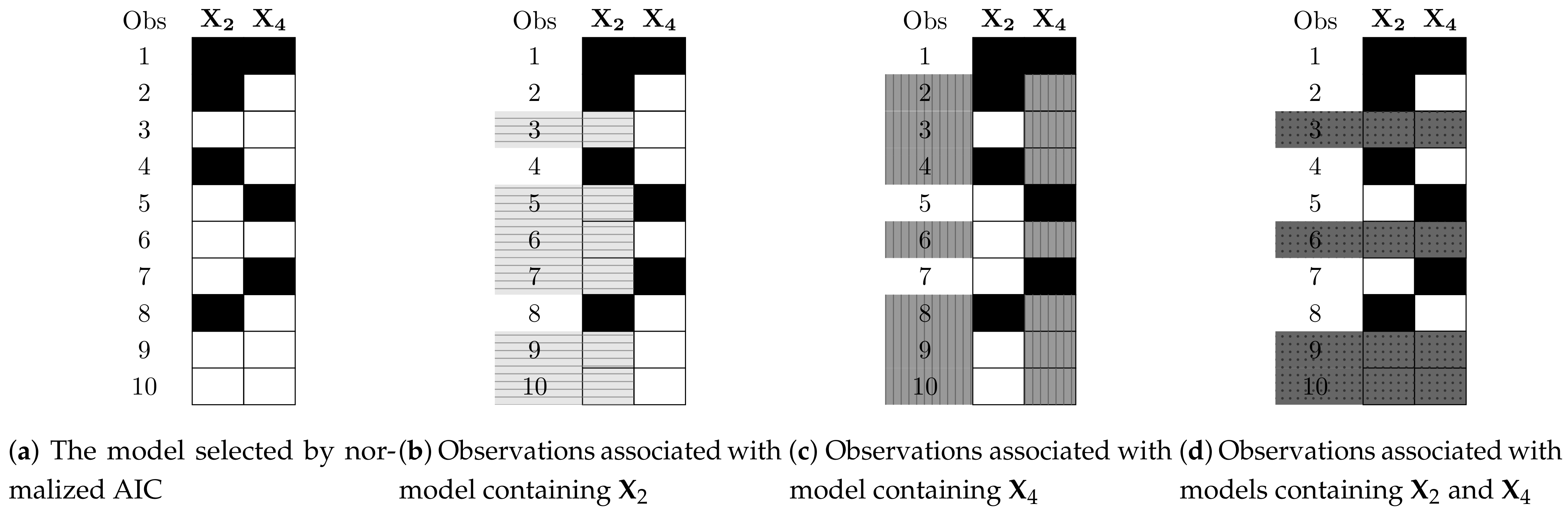
Figure 3.
Comparing the MSE of normalized AIC (NAIC) and other methods, averaged over 100 simulations, and the significance of the differences.
Figure 3.
Comparing the MSE of normalized AIC (NAIC) and other methods, averaged over 100 simulations, and the significance of the differences.

Figure 4.
Comparing the MSE of the methods extending the normalized AIC and normalized AIC (NAIC), averaged over 100 simulations, and the significance of the differences.
Figure 4.
Comparing the MSE of the methods extending the normalized AIC and normalized AIC (NAIC), averaged over 100 simulations, and the significance of the differences.

Figure 5.
Comparing the MSE of the methods extending the normalized AIC and multiple imputation (MI), averaged over 100 simulations, and the significance of the differences.
Figure 5.
Comparing the MSE of the methods extending the normalized AIC and multiple imputation (MI), averaged over 100 simulations, and the significance of the differences.

Figure 6.
Comparing the MSE of the methods extending the normalized AIC to each other, averaged over 100 simulations, and the significance of the differences.
Figure 6.
Comparing the MSE of the methods extending the normalized AIC to each other, averaged over 100 simulations, and the significance of the differences.
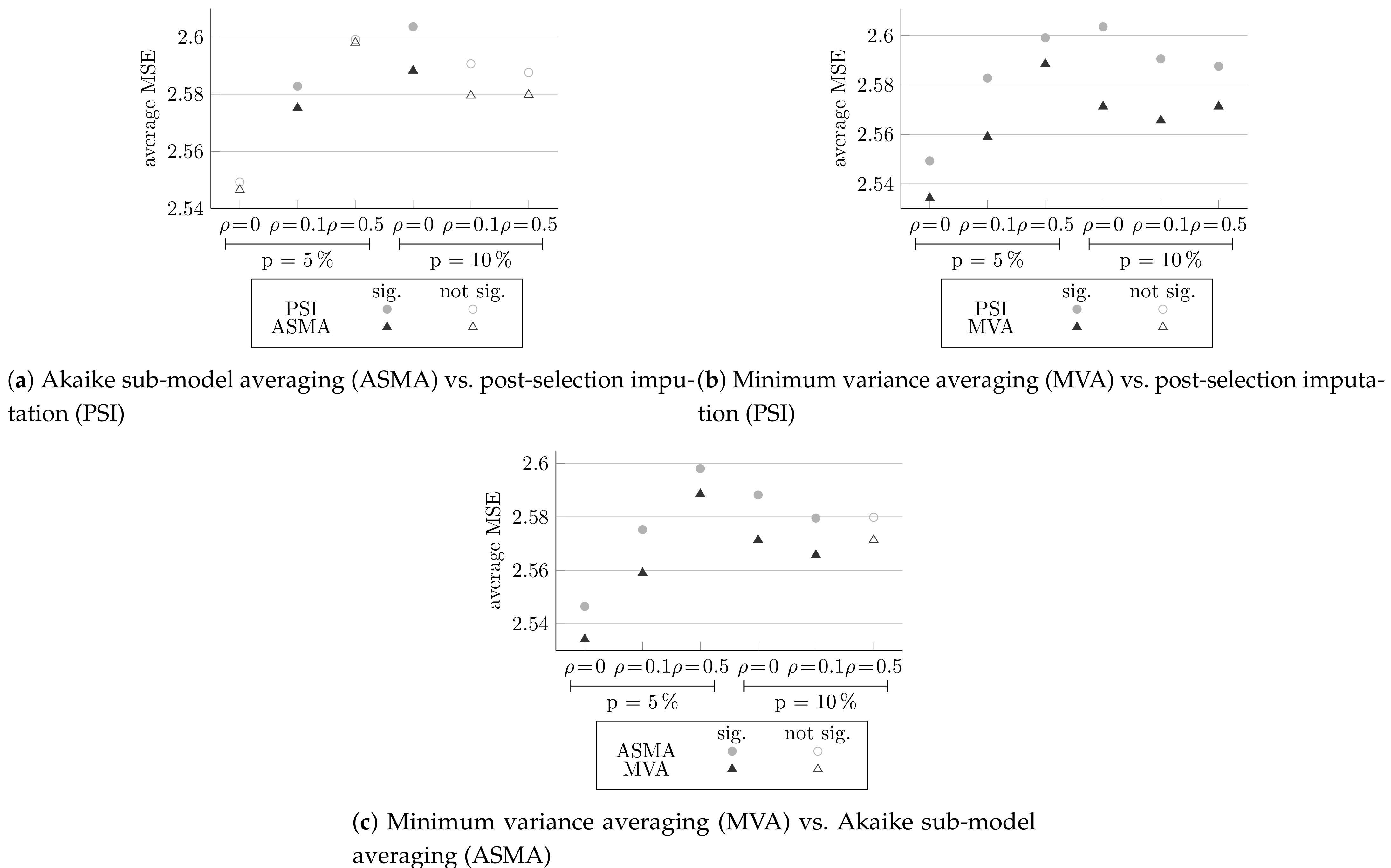
Figure 7.
Comparing the numbers of incorrectly selected variables, for complete case (CC), impute then select (ITS), and normalized BIC (NBIC) methods, averaged over 100 simulations.
Figure 7.
Comparing the numbers of incorrectly selected variables, for complete case (CC), impute then select (ITS), and normalized BIC (NBIC) methods, averaged over 100 simulations.
Publisher’s Note: MDPI stays neutral with regard to jurisdictional claims in published maps and institutional affiliations. |
© 2021 by the authors. Licensee MDPI, Basel, Switzerland. This article is an open access article distributed under the terms and conditions of the Creative Commons Attribution (CC BY) license (https://creativecommons.org/licenses/by/4.0/).
Share and Cite
MDPI and ACS Style
Cohen, N.; Berchenko, Y. Normalized Information Criteria and Model Selection in the Presence of Missing Data. Mathematics 2021, 9, 2474. https://doi.org/10.3390/math9192474
AMA Style
Cohen N, Berchenko Y. Normalized Information Criteria and Model Selection in the Presence of Missing Data. Mathematics. 2021; 9(19):2474. https://doi.org/10.3390/math9192474
Chicago/Turabian StyleCohen, Nitzan, and Yakir Berchenko. 2021. "Normalized Information Criteria and Model Selection in the Presence of Missing Data" Mathematics 9, no. 19: 2474. https://doi.org/10.3390/math9192474
Note that from the first issue of 2016, this journal uses article numbers instead of page numbers. See further details here.