Porous Three-Dimensional Scaffold Generation for 3D Printing


1
Department of Mathematics, Korea University, Seoul 02841, Korea
2
Department of Mathematics, Kangwon National University, Gangwon-do 24341, Korea
*
Author to whom correspondence should be addressed.
Mathematics 2020, 8(6), 946; https://doi.org/10.3390/math8060946
Submission received: 20 May 2020
/
Revised: 3 June 2020
/
Accepted: 4 June 2020
/
Published: 9 June 2020
Abstract
:In this paper, we present an efficient numerical method for arbitrary shaped porous structure generation for 3D printing. A phase-field model is employed for modeling phase separation phenomena of diblock copolymers based on the three-dimensional nonlocal Cahn–Hilliard (CH) equation. The nonlocal CH equation is a fourth-order nonlinear partial differential equation. To efficiently solve the governing equation, an unconditionally gradient stable convex splitting method for temporal discretization with a Fourier spectral method for the spatial discretization is adopted. The standard fast Fourier transform is used to speed up the computation. A new local average concentration function is introduced to the original nonlocal CH equation so that we can locally control the morphology of the structure. The proposed algorithm is simple to implement and complex shaped structures can also be implemented with corresponding signed distance fields. Various numerical tests are performed on simple and complex structures. The computational results demonstrate that the proposed method is efficient to generate irregular porous structures for 3D printing.
1. Introduction
Porosity has many advantages in a variety of fields, including biomaterials, tissue engineering, and clinical medicine. Especially, 3D porous scaffolds have attracted considerable attention in tissue engineering. For instance, bones may be damaged due to accidents or aging in humans; one of the most common methods for severe bone injury is surgical treatment, in which the damaged area is removed and then transplanted for recovery. Because bone is a porous structure, scaffolds with similar porosity distribution and mechanical loading structures need to be studied [1,2].
Porous objects usually have relatively large internal surface areas and are resistant to physical force. Moreover, in the case of a model in which the pores are connected to each other, fluids can flow along them, thereby providing nutrition and cell growth [3]. Therefore, many researches related to generating porous structures have been conducted so far on materials [4], porous sizes [5], architecture [6], topology optimization [7], and 3D printing [8,9] for optimized porous scaffolds. Hollister [10] presented both hierarchical computational topology design and solid free-form fabrication to make 3D anatomic scaffolds with porous structure satisfying the balance between permeability and diffusion. Because creating a porous scaffold that balances mechanical function and material transport is an important issue, how to adjust it efficiently is constantly being studied so far. The authors in [11] used numerical and experimental methods to investigate the influence of the porous structure of triply periodic minimal surface (TPMS) scaffolds on the macroscopic permeability behavior. In addition, advances in 3D printing technology have led to active research into patient-specific structures. As such, the porous scaffolds are closely related to 3D printing. Mohammed et al. [8] examined the creation of unit cells from TPMS renderings as a basis for creating tailored porous structures. In [12], the authors presented a multi-scale porous structure-based lightweight method to make lightweight and strong three-dimensional printed models.
On the one hand, the development of various additive manufacturing technologies [13,14] has made it possible to use various infill technologies for generating 3D objects. These methods are effective for filling the interior of surfaces with porosity. Various methods are used to generate the porosity on surface, such as the Voronoi diagram [15], the Poisson disk sampling [16], and the example-based method [17], etc. Therefore, various combinations of the above methods can be applied to a variety of applications such as designing porosity architecture of bones, for example, by obtaining an internal structure suitable for porous surfaces. On the other hand, there are methods of creating porous objects smoothly using partial differential equations (PDE) to the 3D object itself directly. Creating porous structures using PDE begins with forming patterns on surface. In the previous study, using the reaction-diffusion type PDE, the numerical simulation results with generated patterns on surface were presented in [18]. In this study, the mesh is generated but the interior is not filled, therefore filling inside of object is needed to generate porosity. Then, one can create the object with the similar effect as above. Certain aspects of this approach have been examined implicitly by Jeong et al. [19]. The authors studied numerically a phase-field model for diblock copolymers based on the nonlocal Cahn–Hilliard (CH) equation. The reason why porosity can be obtained is that isosurfaces can be generated using phase-field models. A different average concentration yields a different pattern, i.e., a different porosity by adjusting the phase values.
Therefore, the main purpose of this paper is to use the nonlocal CH equation [19] with a new local average concentration function to generate arbitrary shaped porous structure for 3D printing with space-dependent porous patterns. The CH equation was originally derived from the spinodal decomposition and coarse dynamics of binary alloys. It has been applied to various fields such as image inpainting [20], image segmentation [21], multi-phase flow [22]. Once a signed distance field is given, our method solves the equation and can generate a porous object quickly by using the well-known method, the fast Fourier transform (FFT). Compared with traditional engineering algorithms for generating regular porous architectures, the proposed method allows one to easily adjust parameters to obtain irregular structures with specific volume, density, etc. Regular porous objects are easy to design and fabricate but have shortages such as controlling local pore sizes or distribution of pores. These limitations can be solved through the generation of irregular porous objects [9]. Likewise, these difficulties can be solved by using the modified space-dependent average concentration function in our model.
2. Mathematical Model and Numerical Method
Let be the order parameter. Then, the nonlocal CH equation for modeling a diblock copolymer is given as
where is the domain, and are positive constants, and is the average concentration [19].
In this paper, the nonlocal CH equation with a local average concentration function is proposed to generate arbitrary shaped porous structure for 3D printing:
With the local average concentration function , arbitrary shaped porous structure for 3D printing can be easily generated. When we consider a structure represented by the signed distance function , a local average concentration functions can be defined as follows:
where is a space-dependent function. Figure 1 illustrates a structure in the domain cube.
An unconditionally stable Fourier spectral method is used for the nonlocal CH Equation (1) in 3D space . Fourier spectral method has been applied in many studies [23]. Let be the spatial step size, where , , and are positive even integers. Let be approximations of , where and with the temporal step.
Let be the discrete Fourier transform with a given data , where , and The inverse discrete Fourier transform is
Let
Then,
By using the linearly stabilized splitting scheme [24] to Equation (1), we have
where . Thus, Equation (5) can be transformed into the discrete Fourier space as follows:
Therefore, the following discrete Fourier transform is obtained as follows:
Then, using Equation (4), we get the updated numerical solution as
The standard FFT has been used to speed up the computations [25].
3. Numerical Experiments
In this section, we perform several numerical experiments on various structures and print the resulting 3D models. The interfacial length parameter is defined by mh. This means that there is approximately transition layer width when [26].
3.1. Simple Structures
In this subsection, numerical tests are conducted to generate porous structures inside simple surfaces for which distance functions are well known. The followings are the signed distance functions for a sphere, a cube, a cylinder, and a torus [27]. The periodic nodal surface (PNS) approximation of the Schwarz primitive (P) surface [28,29] is also listed below.
First, let us consider the case that is a constant. The initial phase condition is given as
on the computational domain , where is a random number between and 1. Figure 2a shows the surfaces of the sphere, the cube, the cylinder, the torus, and the P surface with the signed distance functions (7)–(11) from top to bottom. The following parameters are used: , , , , , and . For torus only, the domain is with , and . Figure 2b–d are zero level isosurfaces of numerical solutions at , , and , respectively.
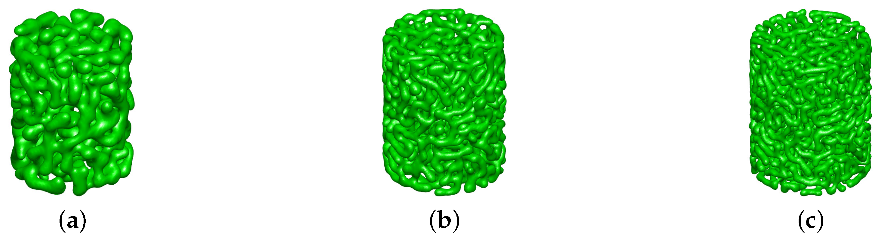
Next, we investigate the effect of parameter on the dynamics of phase separation. The following values are used: , 1000, and 2000, and the rest of the parameters are the same as before. Figure 3a–c show the zero level isosurfaces of at with , 1000, and 2000, respectively. As the value of increases, the structure becomes more detailed.
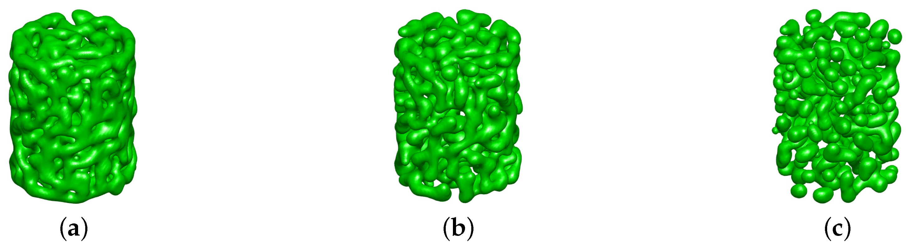
Now, we consider the effect of the local average concentration functions (3). First, the constant average concentration, , , , and are used; and the other parameters are the same as before. Figure 4 show zero level isosurfaces of at with , , and , respectively. According to the values of the local average concentration function, the results show corresponding average concentration morphologies.
Moreover, the following space-dependent average concentration function is used
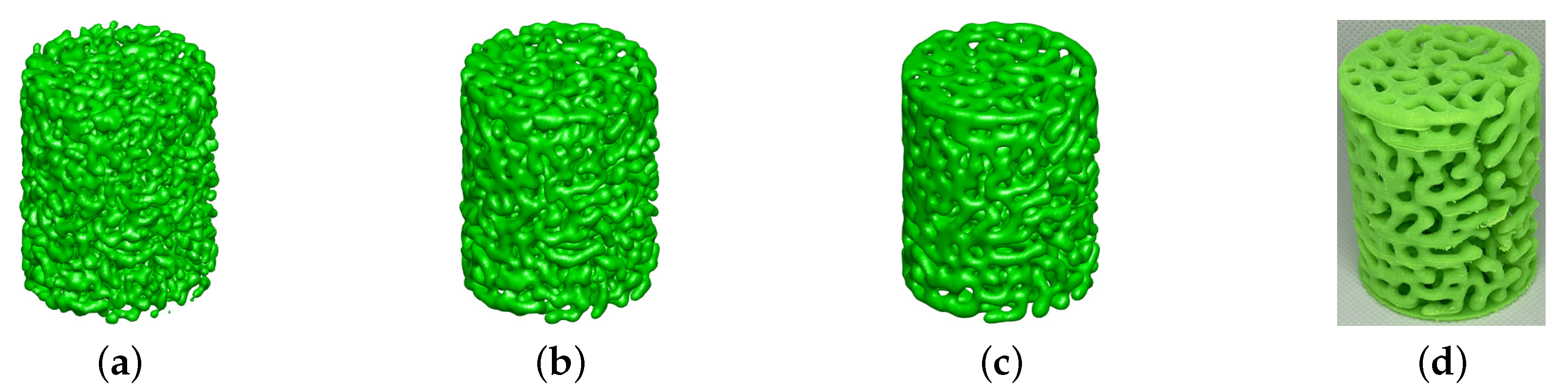
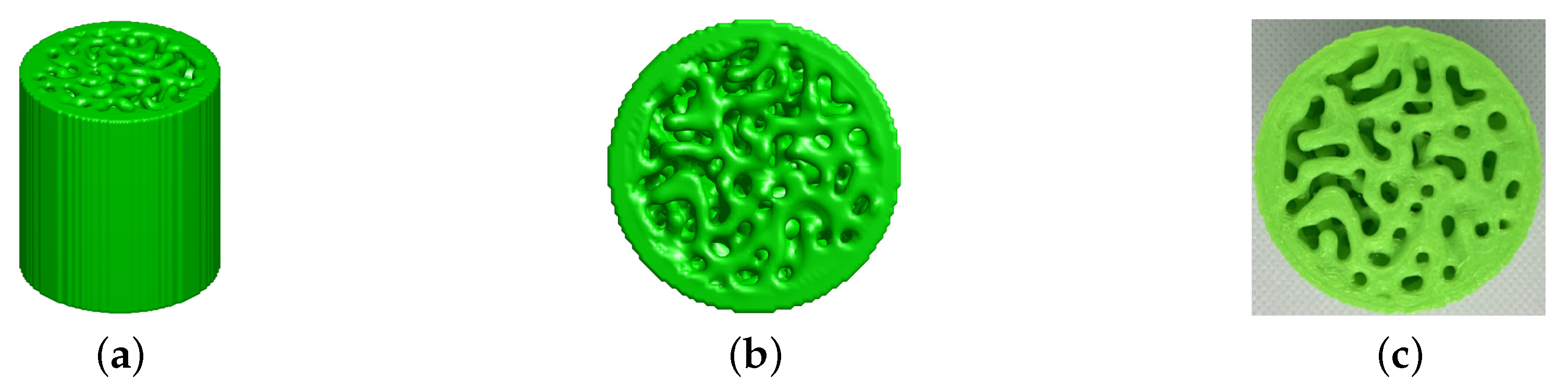
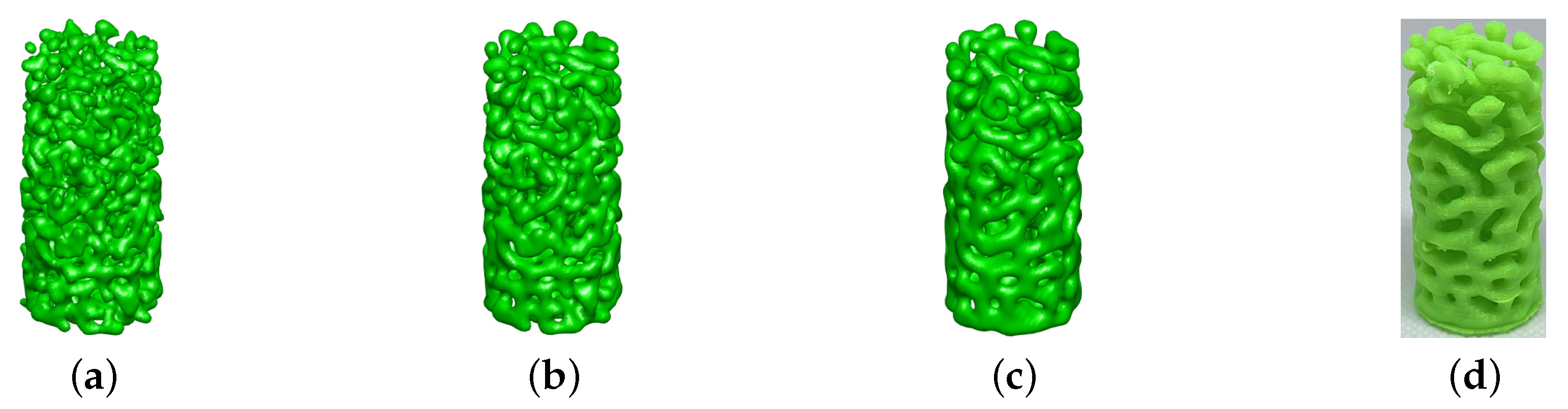
where are inside the cylinder. Here, the parameters are used as follows: , , , and . Figure 5 shows the phase separation of the cylinder structure over time. Figure 5d is a 3D printed model of the structure in Figure 5c. As post-processing, the above cylinder result is covered on the side with and on the bottom thickness. Figure 6 shows the results in Figure 5c with closed cylinder.
Let us consider a cylinder represented by
on the computational domain with a space-dependent average concentration function defined as:
Here, the parameters , , , , , and are used. In Figure 7, there are more porous upwards.
Now, consider a cylinder represented by
on the computational domain with a space-dependent average concentration function defined as:
Here, the following parameters are used: , , , , , and . In Figure 8, there are more porous inside the cylinder.
3.2. Complex Structures
Further examples for complex structures with various average concentration functions are presented. Assume that there is point cloud data of surface for complex structure. First, the Stanford Bunny from the Stanford 3D repository is used as an example for the complex structure. Note that point2trimesh function in MATLAB is used to make a discrete signed distance function for the Stanford bunny. Once the discrete signed distance function is computed, then the procedure is the same as before. Unless otherwise noted, the following initial condition is used for phase separations of complex structure case:
Figure 9a–c show the phase separation on the Stanford Bunny at , , and , respectively. Here, , , , , , , and are used. Furthermore, the following discrete average concentration function is used:
where , , , .
Compared to the constant average function used in the above simulations, the usage of a space-dependent average function produces various patterns in complex structures. For the next step, a similar investigation for the Stanford Armadillo is performed. Figure 10a–c show the phase separation on the Stanford Armadillo at , , and , respectively. Here, , , , , , , , and the same discrete average concentration function Equation (13) are used, where .
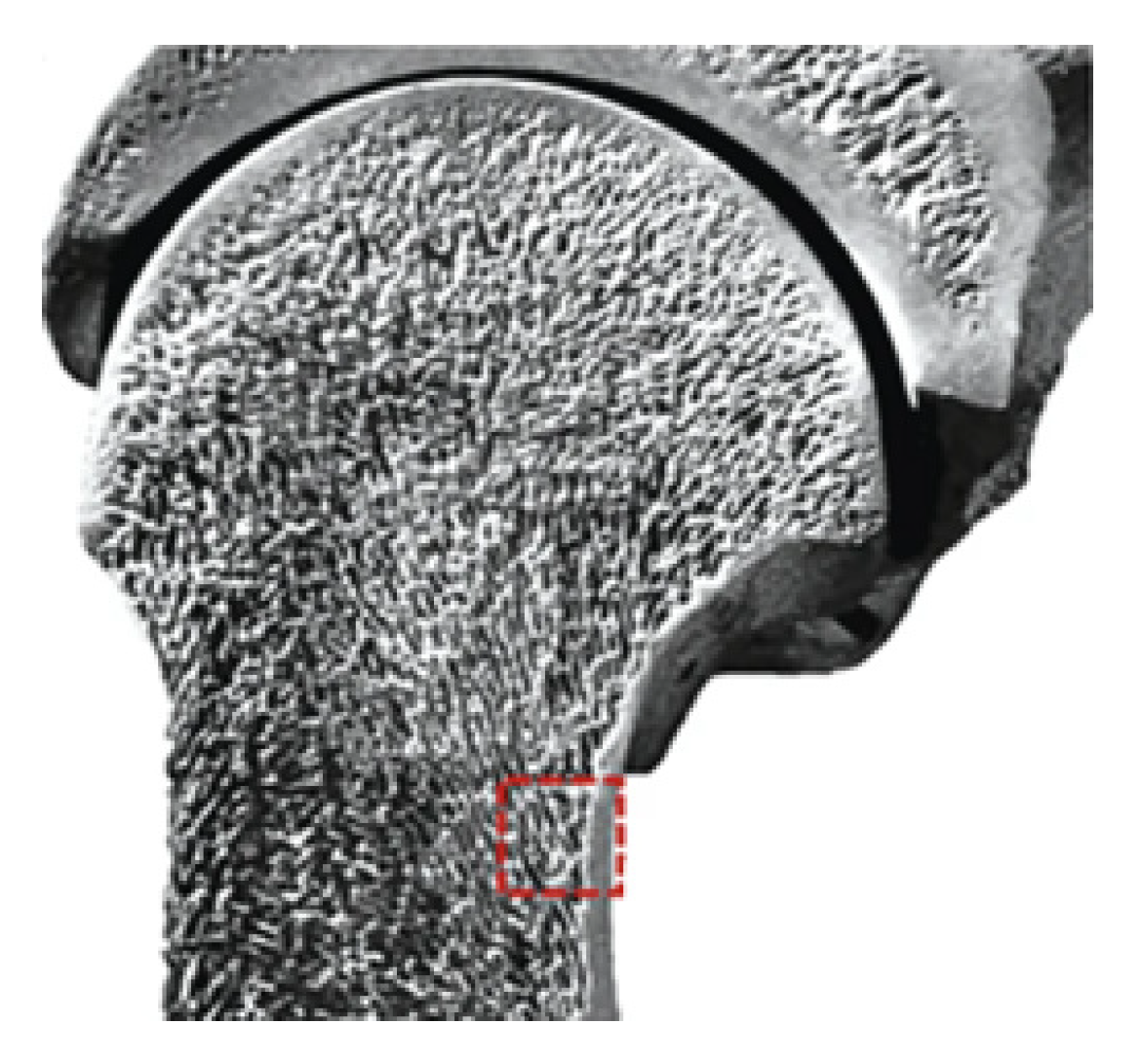
Next, the following examples show that the proposed method for making porous structures can be useful for bone tissue engineering studies because bone is a porous material (see Figure 12). Let us consider a bone and a spine as shown in Figure 13a and Figure 14a.
Similar to the Stanford Bunny, we create a discrete signed distance function using point2trimesh function and use the same initial condition (12). Figure 13b,c illustrate the phase separation on the given bone structure at and , respectively. Here, , , , , , and are used. Moreover, we use the discrete average concentration function (13), where , , , .
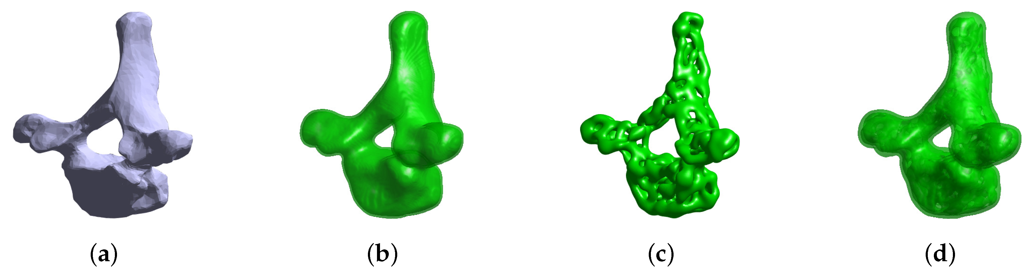
Figure 14b,c illustrate the compact bone made by giving thickness on the given spine, and spongy bone represented by the phase separation on the given spine at . Figure 14d describes the combination of these two structures as post-processing. Here, , , , , , and are used. Moreover, we use the discrete average concentration function (13), where , , , .
3.3. Porous Structure Generation Using TPMS
We consider TPMSs which are widely used for porous scaffold structure in the field of tissue engineering. Numerical simulations are conducted with the signed distance functions of Schwarz primitive (P), Schwarz diamond (D), and Schoen gyroid (G) surface, respectively [28,29]:
as shown in Figure 15. Note that PNS approximations of TPMSs are relaxed and bounded using tanh function in Equations (14)–(16).
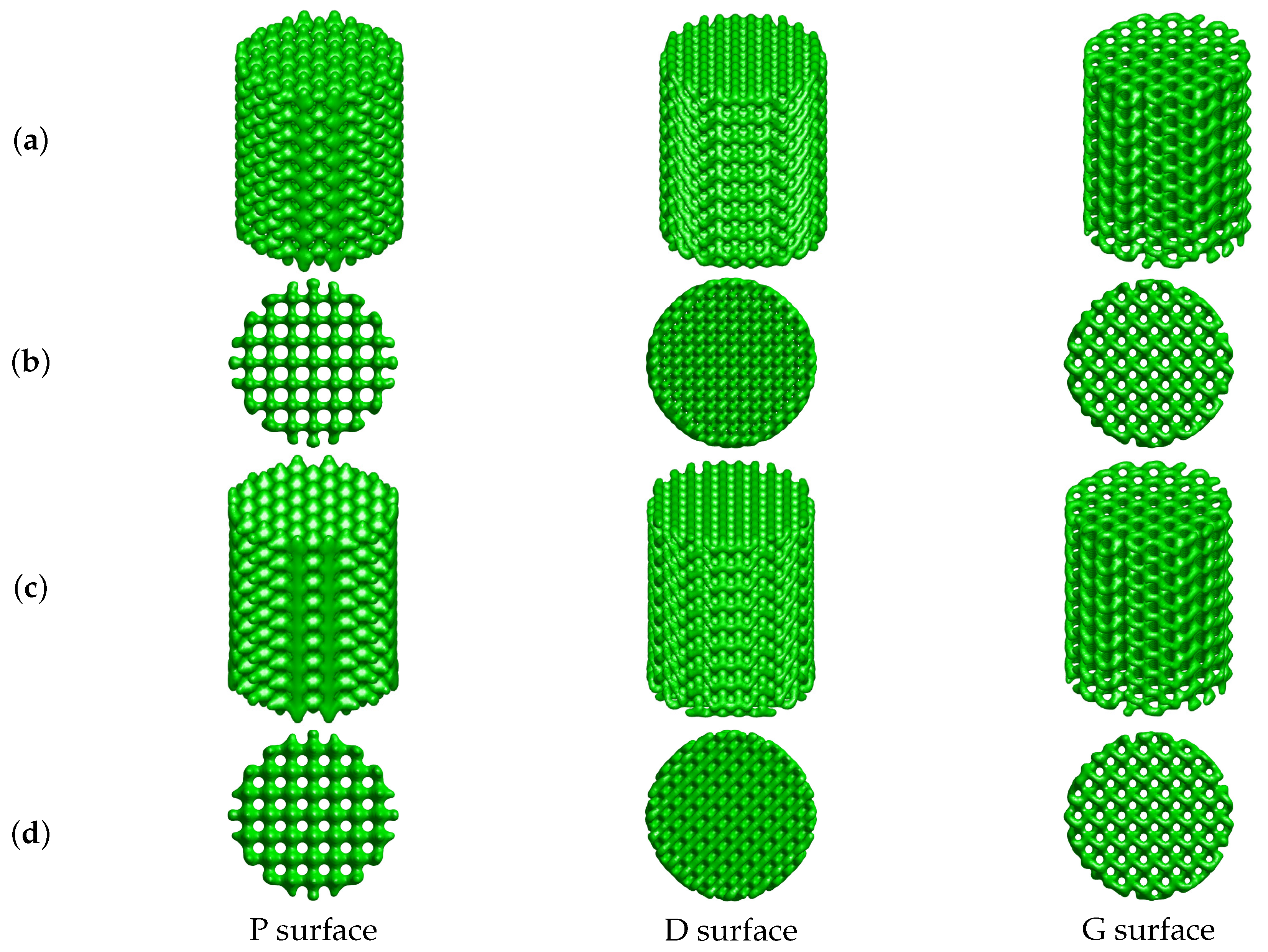
A porous scaffold structure can be created by configuring several TPMSs in the shape of cylinder. In [8], authors made 3D porous scaffolds in a tetrahedral, cubic, and cylindrical configuration using Gyroid and P surfaces. They used commercial programs to make Gyroid and Schwarz P unit cells and create scaffold structures. However, the nonlocal CH equation (2) can be used to make similar results. The following parameters on the computational domain are used: , , , , and . Equation (14) is used as the initial condition in the cylinder (9). Figure 16a–c illustrate the numerical results at , , and , respectively.
Figure 17 shows cylindrical scaffolds using the D surface (15) and G surface (16) with the same parameters as in the previous test. Figure 16 and Figure 17 show the shapes of the scaffolds soften over time.
To smooth the outside of the cylindrical scaffold structure, a post-processing is added after applying Equation (6). Let the whole domain be , the cylindrical domain be , the slightly smaller cylinder be as shown in Figure 18.
First, we make a cylinder with the initial condition and a local average concentration, and save the initial data in the domain . At every iteration, the solution is replaced by the initial value for each . Figure 19 illustrates the numerical results at . Both methods based on the simulation results are compared: On the one hand, Equation (6) is solved on the domain . The results are shown in Figure 19a,b; On the other hand, for is solved and replaced by the initial values. The results are shown in Figure 19c,d. With the second method, we can obtain the cylindrical scaffolds which maintain the original shape of TPMSs inside the cylinder and smooth outside it.
3.4. TPMS Scaffolds Inside Complex Surfaces
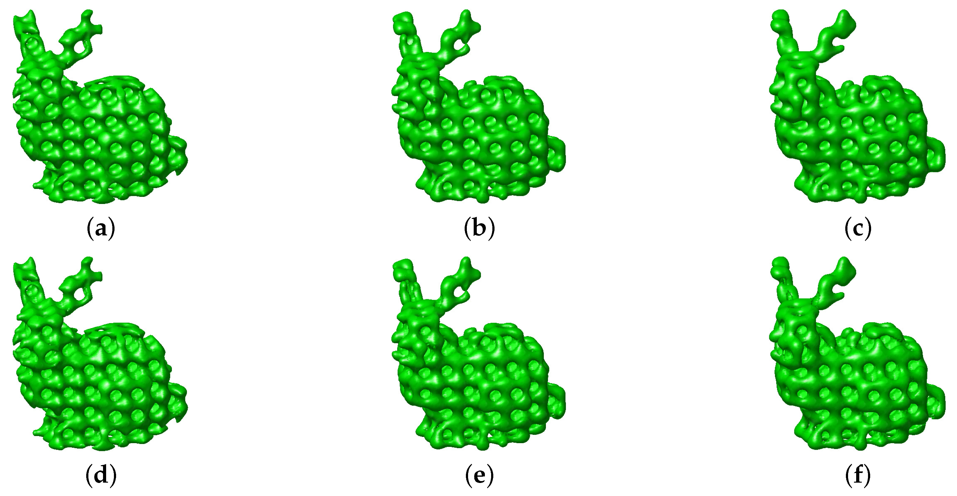
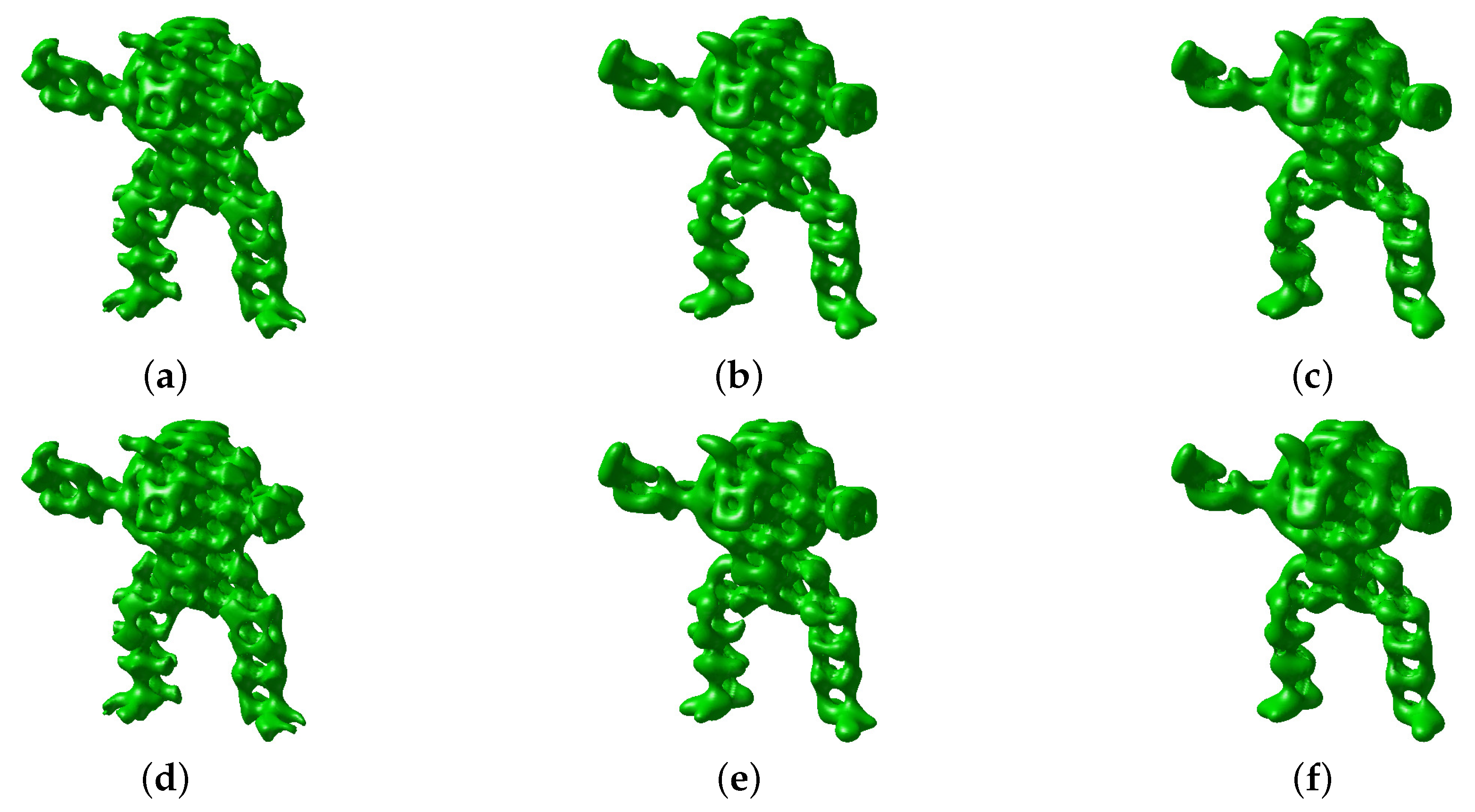
Both methods used in the TPMS section above are applied to the Stanford Bunny and Armadillo. Figure 20 and Figure 21 show snapshots of temporal evolutions with average concentration function Equation (13) for the Stanford Bunny and Armadillo, respectively. All the parameters are the same listed in Section 3.2 except for and .
4. Conclusions
In this paper, the simple numerical method was proposed to generate irregular porous objects using the phase-field model for diblock copolymers based on the nonlocal CH equation. Using the space-dependent local average concentration function, the computational simulation results of generating various typed porous structures were presented. The most important findings are:
- •
- The proposed method can generate porous structures from a solid volume using a distance function.
- •
- The porous structure generating algorithm is simple and easy to implement.
- •
- The proposed algorithm can control pore shapes by the space-dependent average concentration function.
In this article, we focused on the porous structure generation from solid volumes. In future work, we will investigate the generation of porous structure on arbitrary surfaces in three-dimensional space.
Author Contributions
Conceptualization, J.K.; methodology, J.K. and D.J.; software, C.L., D.J., S.Y., and J.K.; validation, C.L. and S.Y.; formal analysis, C.L. and S.Y.; investigation, C.L., D.J., S.Y., and J.K.; writing–original draft preparation, C.L., D.J., S.Y., and J.K.; writing–review and editing, C.L., D.J., S.Y., and J.K.; visualization, C.L. and S.Y.; funding acquisition, J.K., C.L., and D.J. All authors have read and agreed to the published version of the manuscript.
Funding
The first author (C.L.) was supported by Basic Science Research Program through the National Research Foundation of Korea (NRF) funded by the Ministry of Education (NRF-2019R1A6A3A13094308). The author (D.J.) was supported by the National Research Foundation of Korea (NRF) grant funded by the Korea government (MSIP) (NRF-2017R1E1A1A03070953). The corresponding author (J.K.) expresses thanks for the support from the BK21 PLUS program.
Acknowledgments
The authors thank the editor and the reviewers for their constructive and helpful comments on the revision of this article.
Conflicts of Interest
The authors declare no conflict of interest.
References
- Neto, A.; Ferreira, J. Synthetic and marine-derived porous scaffolds for bone tissue engineering. Materials 2018, 11, 1702. [Google Scholar] [CrossRef] [PubMed] [Green Version]
- Kim, T.; Kim, M.; Goh, T.; Lee, J.; Kim, Y.; Yoon, S.; Lee, C. Evaluation of Structural and Mechanical Properties of Porous Artificial Bone Scaffolds Fabricated via Advanced TBA-Based Freeze-Gel Casting Technique. Appl. Sci. 2019, 9, 1965. [Google Scholar] [CrossRef] [Green Version]
- Scheffler, M.; Colombo, P. Cellular Ceramics: Structure, Manufacturing, Properties and Applications; John Wiley & Sons: Hoboken, NJ, USA, 2006. [Google Scholar]
- Gajendiran, M.; Choi, J.; Kim, S.J.; Kim, K.; Shin, H.; Koo, H.J.; Kim, K. Conductive biomaterials for tissue engineering applications. J. Ind. Eng. Chem. 2017, 51, 12–26. [Google Scholar] [CrossRef]
- Tang, W.; Lin, D.; Yu, Y.; Niu, H.; Guo, H.; Yuan, Y.; Liu, C. Bioinspired trimodal macro/micro/nano-porous scaffolds loading rhBMP-2 for complete regeneration of critical size bone defect. Acta Biomater. 2016, 32, 309–323. [Google Scholar] [CrossRef] [PubMed]
- Cipitria, A.; Lange, C.; Schell, H.; Wagermaier, W.; Reichert, J.C.; Hutmacher, D.W.; Fratzl, P.; Duda, G.N. Porous scaffold architecture guides tissue formation. J. Bone Miner. Res. 2012, 27, 1275–1288. [Google Scholar] [CrossRef] [PubMed]
- Zhang, P.; Toman, J.; Yu, Y.; Biyikli, E.; Kirca, M.; Chmielus, M.; To, A.C. Efficient design-optimization of variable-density hexagonal cellular structure by additive manufacturing: Theory and validation. J. Manuf. Sci. Eng. 2015, 137, 021004. [Google Scholar] [CrossRef]
- Mohammed, M.I.; Badwal, P.S.; Gibson, I. Design and fabrication considerations for three dimensional scaffold structures. In Proceedings of the International Conference on Design and Technologyy, KEG, Geelong, Australia, 5–8 December 2016; pp. 120–126. [Google Scholar]
- Kou, X.; Tan, S. A simple and effective geometric representation for irregular porous structure modeling. Comput. Aided Des. 2010, 42, 930–941. [Google Scholar] [CrossRef] [Green Version]
- Hollister, S.J. Porous scaffold design for tissue engineering. Nat. Mater. 2005, 4, 518. [Google Scholar] [CrossRef]
- Castro, A.; Pires, T.; Santos, J.; Gouveia, B.; Fernandes, P. Permeability versus Design in TPMS Scaffolds. Materials 2019, 12, 1313. [Google Scholar] [CrossRef] [Green Version]
- Hu, J.; Wang, S.; Wang, Y.; Li, F.; Luo, Z. A lightweight methodology of 3D printed objects utilizing multi-scale porous structures. Vis. Comput. 2019, 35, 949–959. [Google Scholar] [CrossRef]
- Song, Y.; Yang, Z.; Liu, Y.; Deng, J. Function representation based slicer for 3d printing. Comput. Aided Geom. Des. 2018, 62, 276–293. [Google Scholar] [CrossRef]
- Mao, Y.; Wu, L.; Yan, D.M.; Guo, J.; Chen, C.W.; Chen, B. Generating hybrid interior structure for 3D printing. Comput. Aided Geom. Des. 2018, 62, 63–72. [Google Scholar] [CrossRef]
- Wang, X.; Ying, X.; Liu, Y.J.; Xin, S.Q.; Wang, W.; Gu, X.; Mueller-Wittig, W.; He, Y. Intrinsic computation of centroidal Voronoi tessellation (CVT) on meshes. Comput. Aided Des. 2015, 58, 51–61. [Google Scholar] [CrossRef]
- Corsini, M.; Cignoni, P.; Scopigno, R. Efficient and flexible sampling with blue noise properties of triangular meshes. IEEE Trans. Vis. Comput. Graph. 2012, 18, 914–924. [Google Scholar] [CrossRef] [PubMed] [Green Version]
- Schumacher, C.; Thomaszewski, B.; Gross, M. Stenciling: Designing Structurally-Sound Surfaces with Decorative Patterns. Comput. Graph. Forum. 2016, 35, 101–110. [Google Scholar] [CrossRef]
- Turk, G. Generating textures on arbitrary surfaces using reaction-diffusion. In ACM SIGGRAPH Computer Graphics; ACM: New York, NY, USA, 1991; Volume 25, pp. 289–298. [Google Scholar]
- Jeong, D.; Kim, J. Microphase separation patterns in diblock copolymers on curved surfaces using a nonlocal Cahn–Hilliard equation. Eur. Phys. J. E 2015, 38, 117. [Google Scholar] [CrossRef]
- Bertozzi, A.L.; Esedoglu, S.; Gillette, A. Inpainting of binary images using the Cahn–Hilliard equation. IEEE Trans. Image Process. 2006, 16, 285–291. [Google Scholar] [CrossRef]
- Chalupeckỳ, V. Numerical studies of Cahn–Hilliard equation and applications in image processing. In Proceedings of the Czech–Japanese Seminar in Applied Mathematics, Praha, Czech Republic, 4–7 August 2004; pp. 10–22. [Google Scholar]
- Boyer, F.; Lapuerta, C.; Minjeaud, S.; Piar, B.; Quintard, M. Cahn–Hilliard/Navier–Stokes model for the simulation of three-phase flows. Transp. Porous Media 2010, 82, 463–483. [Google Scholar] [CrossRef]
- Li, Y.; Wang, J.; Lu, B.; Jeong, D.; Kim, J. Multicomponent volume reconstruction from slice data using a modified multicomponent Cahn–Hilliard system. Pattern Recognit. 2019, 93, 124–133. [Google Scholar] [CrossRef]
- Eyre, D.J. An unconditionally stable one-step scheme for gradient systems. 1998, 1–15, Unpublished article. [Google Scholar]
- Shen, J.; Tang, T.; Wang, L.L. Spectral Methods: Algorithms, Analysis and Applications; Springer Science & Business Media: Berlin/Heidelberg, Germany, 2011; Volume 41. [Google Scholar]
- Kim, J. Phase-field models for multi-component fluid flows. Commun. Comput. Phys. 2012, 12, 613–661. [Google Scholar] [CrossRef]
- Shin, J.; Jeong, D.; Kim, J. A conservative numerical method for the Cahn–Hilliard equation in complex domains. J. Comput. Phys. 2011, 230, 7441–7455. [Google Scholar] [CrossRef]
- Yoo, D.J. Computer-aided porous scaffold design for tissue engineering using triply periodic minimal surfaces. Int. J. Precis. Eng. Manuf. 2011, 12, 61–71. [Google Scholar] [CrossRef]
- Lee, H.G.; Park, J.; Yoon, S.; Lee, C.; Kim, J. Mathematical Model and Numerical Simulation for Tissue Growth on Bioscaffolds. Appl. Sci. 2019, 9, 4058. [Google Scholar] [CrossRef] [Green Version]
- Gong, T.; Xie, J.; Liao, J.; Zhang, T.; Lin, S.; Lin, Y. Nanomaterials and bone regeneration. Bone Res. 2015, 3, 15029. [Google Scholar] [CrossRef]
Figure 1.
Schematic diagram illustrating a volume in the cubic domain.

Figure 2.
Sphere, cube, cylinder, torus, P surface from top to bottom. (a) Surfaces and (b–d) zero level isosurfaces of at , and , respectively, with an initial condition .
Figure 2.
Sphere, cube, cylinder, torus, P surface from top to bottom. (a) Surfaces and (b–d) zero level isosurfaces of at , and , respectively, with an initial condition .

Figure 3.
(a–c) are zero level isosurfaces of at with , 1000, and 2000, respectively, and .

Figure 4.
(a–c) are zero level isosurfaces of at with , , and , respectively, and .

Figure 5.
Zero level isosurfaces of at (a) , (b) , and (c) . (d) 3D printed model of zero level isosurfaces of at .
Figure 5.
Zero level isosurfaces of at (a) , (b) , and (c) . (d) 3D printed model of zero level isosurfaces of at .

Figure 6.
(a,b) Zero level isosurfaces of with closed cylinder at , and (c) its corresponding 3D printed model.
Figure 6.
(a,b) Zero level isosurfaces of with closed cylinder at , and (c) its corresponding 3D printed model.

Figure 7.
Zero level isosurfaces of with at (a) , (b) , and (c) . (d) 3D printed model of zero level isosurfaces of at .
Figure 7.
Zero level isosurfaces of with at (a) , (b) , and (c) . (d) 3D printed model of zero level isosurfaces of at .

Figure 8.
Temporal phase separation with at (a) , (b) , and (c) . (d) 3D printed model of zero level isosurfaces of at .
Figure 8.
Temporal phase separation with at (a) , (b) , and (c) . (d) 3D printed model of zero level isosurfaces of at .

Figure 9.
(a–c) are snapshots of phase separation with average concentration function Equation (13) on the Stanford Bunny at , , and , respectively.
Figure 9.
(a–c) are snapshots of phase separation with average concentration function Equation (13) on the Stanford Bunny at , , and , respectively.

Figure 10.
(a–c) are snapshots of phase separation with average concentration function Equation (13) on the Stanford Armadillo at , , and , respectively.
Figure 10.
(a–c) are snapshots of phase separation with average concentration function Equation (13) on the Stanford Armadillo at , , and , respectively.


Figure 12.
Porous structure inside the bone. Reprinted with permission from Gong et al. [30]. Copyright 2015, Springer Nature.
Figure 12.
Porous structure inside the bone. Reprinted with permission from Gong et al. [30]. Copyright 2015, Springer Nature.

Figure 13.
(a) Bone structure. (b) and (c) are snapshots of phase separation with average concentration function Equation (13) at and , respectively.
Figure 13.
(a) Bone structure. (b) and (c) are snapshots of phase separation with average concentration function Equation (13) at and , respectively.

Figure 14.
(a) Spine. (b) Compact bone. (c) Spongy bone represented by the snapshot of phase separation with average concentration function Equation (13) at . (d) Combination of (b) and (c).
Figure 14.
(a) Spine. (b) Compact bone. (c) Spongy bone represented by the snapshot of phase separation with average concentration function Equation (13) at . (d) Combination of (b) and (c).

Figure 15.
Triply periodic minimal surfaces: P, D, and G.

Figure 16.
Cylindrical scaffolds using the P surface. Snapshots of phase separation at (a) , (b) , and (c) .
Figure 16.
Cylindrical scaffolds using the P surface. Snapshots of phase separation at (a) , (b) , and (c) .

Figure 17.
Cylindrical scaffolds using the (a,b) D and (c,d) G surfaces. Snapshots of phase separation at and from left to right.
Figure 17.
Cylindrical scaffolds using the (a,b) D and (c,d) G surfaces. Snapshots of phase separation at and from left to right.

Figure 18.
Schematic diagram illustrating a surface in the cubic domain .

Figure 19.
Comparison between phase separation of two methods at : (a,b) Equation (6) is solved on the domain ; (c,d) for is updated with the initial condition.
Figure 19.
Comparison between phase separation of two methods at : (a,b) Equation (6) is solved on the domain ; (c,d) for is updated with the initial condition.

Figure 20.
(a–c) are snapshots of phase separation on the Stanford Bunny at , , and , respectively. (d–f) are snapshots of phase separation with replacing initial values inside the object at , , and , respectively. Here, the local average concentration function Equation (13) is used.
Figure 20.
(a–c) are snapshots of phase separation on the Stanford Bunny at , , and , respectively. (d–f) are snapshots of phase separation with replacing initial values inside the object at , , and , respectively. Here, the local average concentration function Equation (13) is used.

Figure 21.
(a–c) are snapshots of phase separation on the Stanford Armadillo at , , and , respectively. (d–f) are snapshots of phase separation with replacing initial values inside the object at , , and , respectively. Here, the local average concentration function Equation (13) is used.
Figure 21.
(a–c) are snapshots of phase separation on the Stanford Armadillo at , , and , respectively. (d–f) are snapshots of phase separation with replacing initial values inside the object at , , and , respectively. Here, the local average concentration function Equation (13) is used.

© 2020 by the authors. Licensee MDPI, Basel, Switzerland. This article is an open access article distributed under the terms and conditions of the Creative Commons Attribution (CC BY) license (http://creativecommons.org/licenses/by/4.0/).
Share and Cite
MDPI and ACS Style
Lee, C.; Jeong, D.; Yoon, S.; Kim, J. Porous Three-Dimensional Scaffold Generation for 3D Printing. Mathematics 2020, 8, 946. https://doi.org/10.3390/math8060946
AMA Style
Lee C, Jeong D, Yoon S, Kim J. Porous Three-Dimensional Scaffold Generation for 3D Printing. Mathematics. 2020; 8(6):946. https://doi.org/10.3390/math8060946
Chicago/Turabian StyleLee, Chaeyoung, Darae Jeong, Sungha Yoon, and Junseok Kim. 2020. "Porous Three-Dimensional Scaffold Generation for 3D Printing" Mathematics 8, no. 6: 946. https://doi.org/10.3390/math8060946
Note that from the first issue of 2016, this journal uses article numbers instead of page numbers. See further details here.