An Efficient Conjugate Gradient Method for Convex Constrained Monotone Nonlinear Equations with Applications †


1
KMUTTFixed Point Research Laboratory, SCL 802 Fixed Point Laboratory, Science Laboratory Building, Department of Mathematics, Faculty of Science, King Mongkut’s University of Technology Thonburi (KMUTT), 126 Pracha-Uthit Road, Bang Mod, Thrung Khru, Bangkok 10140, Thailand
2
Department of Mathematical Sciences, Faculty of Physical Sciences, Bayero University, Kano 700241, Nigeria
3
Center of Excellence in Theoretical and Computational Science (TaCS-CoE), Science Laboratory Building, King Mongkut’s University of Technology Thonburi (KMUTT), 126 Pracha-Uthit Road, Bang Mod, Thrung Khru, Bangkok 10140, Thailand
4
Department of Medical Research, China Medical University Hospital, China Medical University, Taichung 40402, Taiwan
5
Department of Mathematics, Faculty of Science, Gombe State University, Gombe 760214, Nigeria
*
Author to whom correspondence should be addressed.
†
This project was supported by Petchra Pra Jom Klao Doctoral Academic Scholarship for Ph.D. Program at KMUTT. Moreover, this project was partially supported by the Thailand Research Fund (TRF) and the King Mongkut’s University of Technology Thonburi (KMUTT) under the TRF Research Scholar Award (Grant No. RSA6080047).
Mathematics 2019, 7(9), 767; https://doi.org/10.3390/math7090767
Submission received: 29 June 2019
/
Revised: 30 July 2019
/
Accepted: 6 August 2019
/
Published: 21 August 2019
(This article belongs to the Special Issue Iterative Methods for Solving Nonlinear Equations and Systems)
Abstract
:This research paper proposes a derivative-free method for solving systems of nonlinear equations with closed and convex constraints, where the functions under consideration are continuous and monotone. Given an initial iterate, the process first generates a specific direction and then employs a line search strategy along the direction to calculate a new iterate. If the new iterate solves the problem, the process will stop. Otherwise, the projection of the new iterate onto the closed convex set (constraint set) determines the next iterate. In addition, the direction satisfies the sufficient descent condition and the global convergence of the method is established under suitable assumptions. Finally, some numerical experiments were presented to show the performance of the proposed method in solving nonlinear equations and its application in image recovery problems.
Keywords:
nonlinear monotone equations; conjugate gradient method; projection method; signal processingMSC:
65K05; 90C52; 90C56; 92C551. Introduction
In this paper, we consider the following constrained nonlinear equation
where is continuous and monotone. The constraint set is nonempty, closed and convex.
Monotone equations appear in many applications [1,2,3], for example, the subproblems in the generalized proximal algorithms with Bregman distance [4], reformulation of some -norm regularized problems arising in compressive sensing [5] and variational inequality problems are also converted into nonlinear monotone equations via fixed point maps or normal maps [6], (see References [7,8,9] for more examples). Among earliest methods for the case is the hyperplane projection Newton method proposed by Solodov and Svaiter in Reference [10]. Subsequently, many methods were proposed by different authors. Among the popular methods are spectral gradient methods [11,12], quasi-Newton methods [13,14,15] and conjugate gradient methods (CG) [16,17].
To solve the constrained case (1), the work of Solodov and Svaiter was extended by Wang et al. [18] which also involves solving a linear system in each iteration but it was shown later by some authors that the computation of the linear system is not necessary. For examples, Xiao and Zhu [19] presented a CG method, which is a combination the well known CG-DESCENT method in Reference [20] with the projection strategy by Solodov and Svaiter. Liu et al. [21] presented two CG method with sufficiently descent directions. In Reference [22], a modified version of the method in Reference [19] was presented by Liu and Li. The modification improves the numerical performance of the method in Reference [19]. Another extension of the Dai and Kou (DK) CG method combined with the projection method to solve (1) was proposed by Ding et al. in Reference [23]. Just recently, to popularize the Dai-Yuan (DY) CG method, Liu and Feng [24] modified the DY such that the direction will be sufficiently descent. A new hybrid spectral gradient projection method for solving convex constraints nonlinear monotone equations was proposed by Awwal et al. in Reference [25]. The method is a convex combination of two different positive spectral parameters together with the projection strategy. In addition, Abubakar et al. extended the method in Reference [17] to solve (1) and also solve some sparse signal recovery problems.
Inspired by some the above methods, we propose a descent conjugate gradient method to solve problem (1). Under appropriate assumptions, the global convergence is established. Preliminary numerical experiments were given to compare the proposed method with existing methods to solve nonlinear monotone equations and some signal and image reconstruction problems arising from compressive sensing.
The remaining part of this paper is organized as follows. In Section 2, we state the proposed algorithm as well as its convergence analysis. Finally, Section 3 reports some numerical results to show the performance of the proposed method in solving Equation (1), signal recovery problems and image restoration problems.
2. Algorithm: Motivation and Convergence Result
This section starts by defining the projection map together with some of its properties.
Definition 1.
Let be a nonempty closed convex set. Then for any , its projection onto Ψ, denoted by , is defined by
Moreover, is nonexpansive, That is,
All through this article, we assume the followings
- ()
- The mapping F is monotone, that is,
- ()
- The mapping F is Lipschitz continuous, that is there exists a positive constant L such that
- ()
- The solution set of (1), denoted by , is nonempty.
An important property that methods for solving Equation (1) must possess is that the direction satisfy
where is a constant. The inequality (3) is called sufficient descent property if is the gradient vector of a real valued function .
In this paper, we propose the following search direction
where
and is determined such that Equation (3) is satisfied. It is easy to see that for , the equation holds with . Now for ,
aking we have
Thus, the direction defined by (4) satisfy condition (3) where .
To prove the global convergence of Algorithm 1, the following lemmas are needed.
| Algorithm 1: (DCG) |
| Step 0. Given an arbitrary initial point , parameters , , and set . Step 1. If , stop, otherwise go to Step 2. Step 2. Compute using Equation (4). Step 3. Compute the step size such that Step 4. Set . If and , stop. Else compute where Step 5. Let and go to Step 1. |
Lemma 1.
Lemma 2.
Suppose that assumptions ()–() holds, then the sequences and generated by Algorithm 1 (CGD) are bounded. Moreover, we have
and
Proof.
We will start by showing that the sequences and are bounded. Suppose , then by monotonicity of F, we get
Also by definition of and the line search (8), we have
So, we have
Thus the sequence is non increasing and convergent and hence is bounded. Furthermore, from Equation (13), we have
and we can deduce recursively that
Then from Assumption (), we obtain
If we let , then the sequence is bounded, that is,
The boundedness of the sequence together with Equations (15) and (16), implies the sequence is bounded.
Since is bounded, then for any , the sequence is also bounded, that is, there exists a positive constant such that
This together with Assumption () yields
Equation (17) implies
However, using Equation (2), the definition of and the Cauchy-Schwartz inequality, we have
which yields
☐
Equation (9) and definition of implies that
Lemma 3.
Suppose is generated by Algorithm 1 (CGD), then there exist such the
Proof.
By definition of and Equation (15)
Letting , we have the desired result. ☐
Theorem 1.
Suppose that assumptions ()–() hold and let the sequence be generated by Algorithm 1, then
Proof.
To prove the Theorem, we consider two cases;
Case 1
Suppose we have Then by continuity of F, the sequence has some accumulation point such that Because converges and is an accumulation point of , therefore converges to .
Case 2
3. Numerical Examples
This section gives the performance of the proposed method with existing methods such as PCG and PDY proposed in References [22,24], respectively, to solve monotone nonlinear equations using 9 benchmark test problems. Furthermore Algorithm 1 is applied to restore a blurred image. All codes were written in MATLAB R2018b and run on a PC with intel COREi5 processor with 4 GB of RAM and CPU 2.3 GHZ. All runs were stopped whenever
The parameters chosen for the existing algorithm are as follows:
PCG method: All parameters are chosen as in Reference [22].
PDY method: All parameters are chosen as in Reference [24].
Algorithm 1: We have tested several values of and found that gives the best result. In addition, to implement most of the optimization algorithms, the parameter is chosen as a very small number. Therefore, we chose and for the implementation of the proposed algorithm.
We test 9 different problems with dimensions ranging from and 6 initial points: , , , , , . In Table 1, Table 2, Table 3, Table 4, Table 5, Table 6, Table 7, Table 8 and Table 9, the number of iterations (ITER), number of function evaluations (FVAL), CPU time in seconds (TIME) and the norm at the approximate solution (NORM) were reported. The symbol ‘−’ is used when the number of iterations exceeds 1000 and/or the number of function evaluations exceeds 2000.
The test problems are listed below, where the function F is taken as .
Problem 1
Problem 2
Problem 3
It is clear that Problem 3 is nonsmooth at .
Problem 4
Problem 5
Problem 6
Problem 7
Problem 8
Problem 9
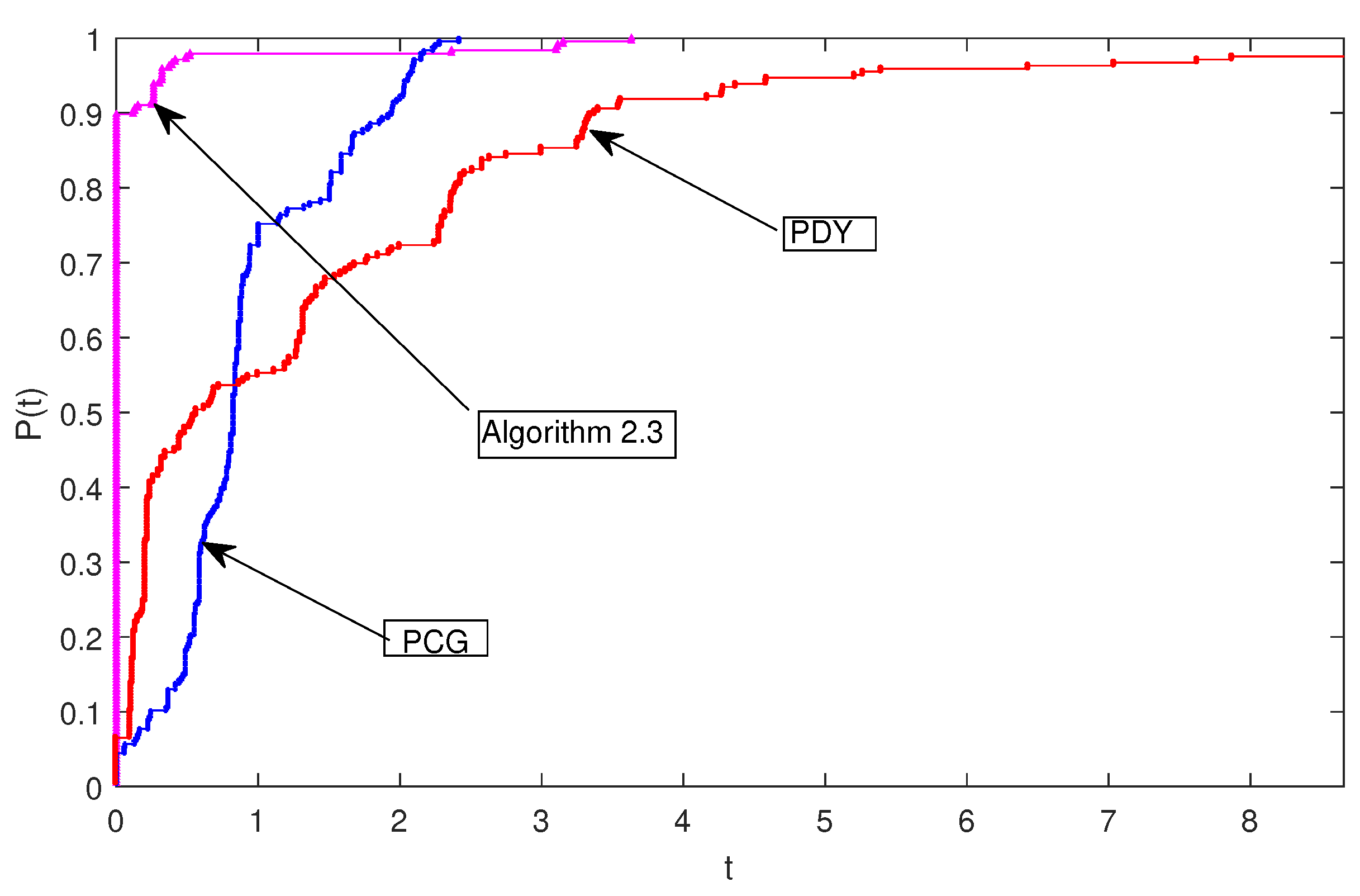
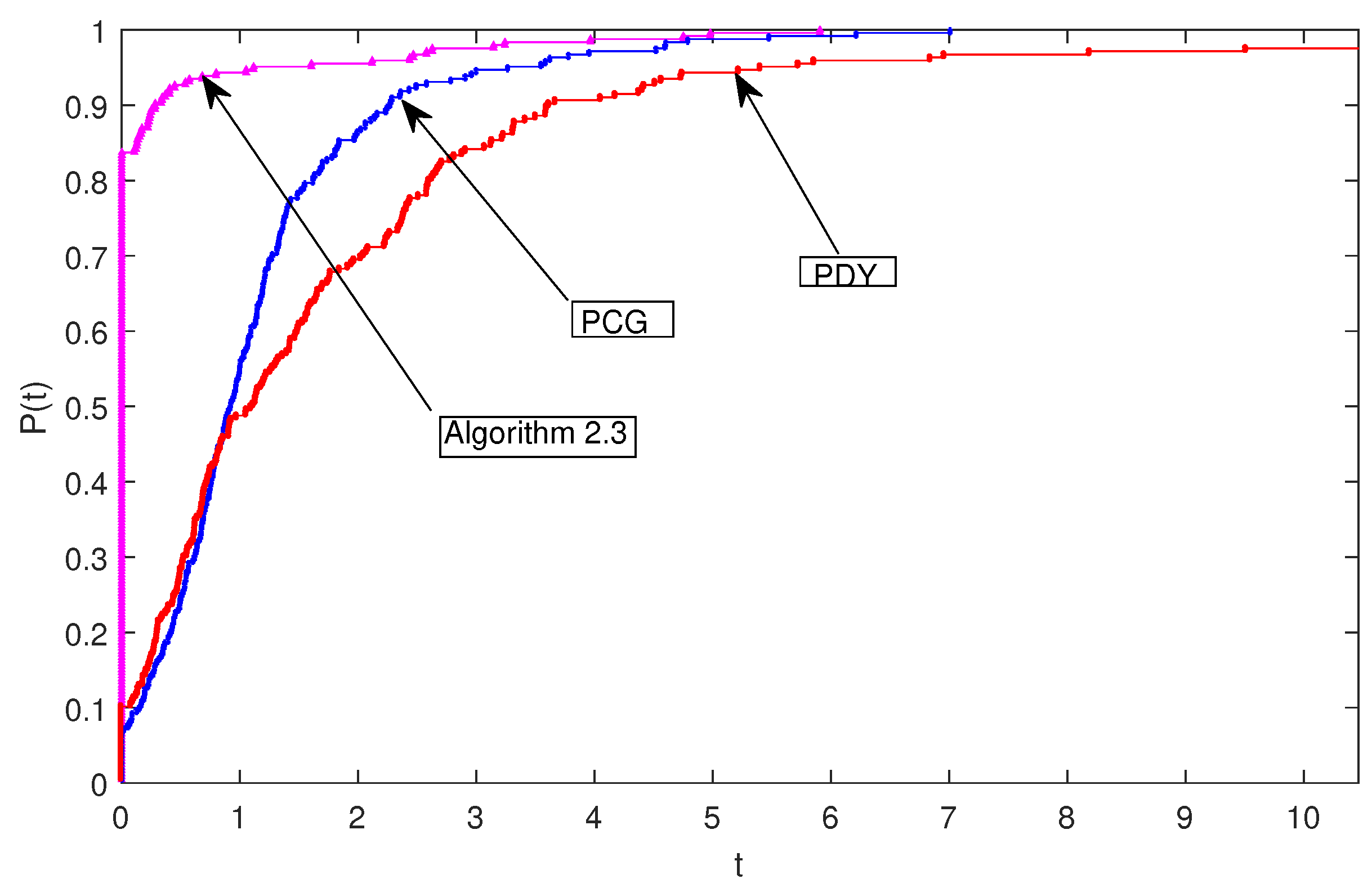
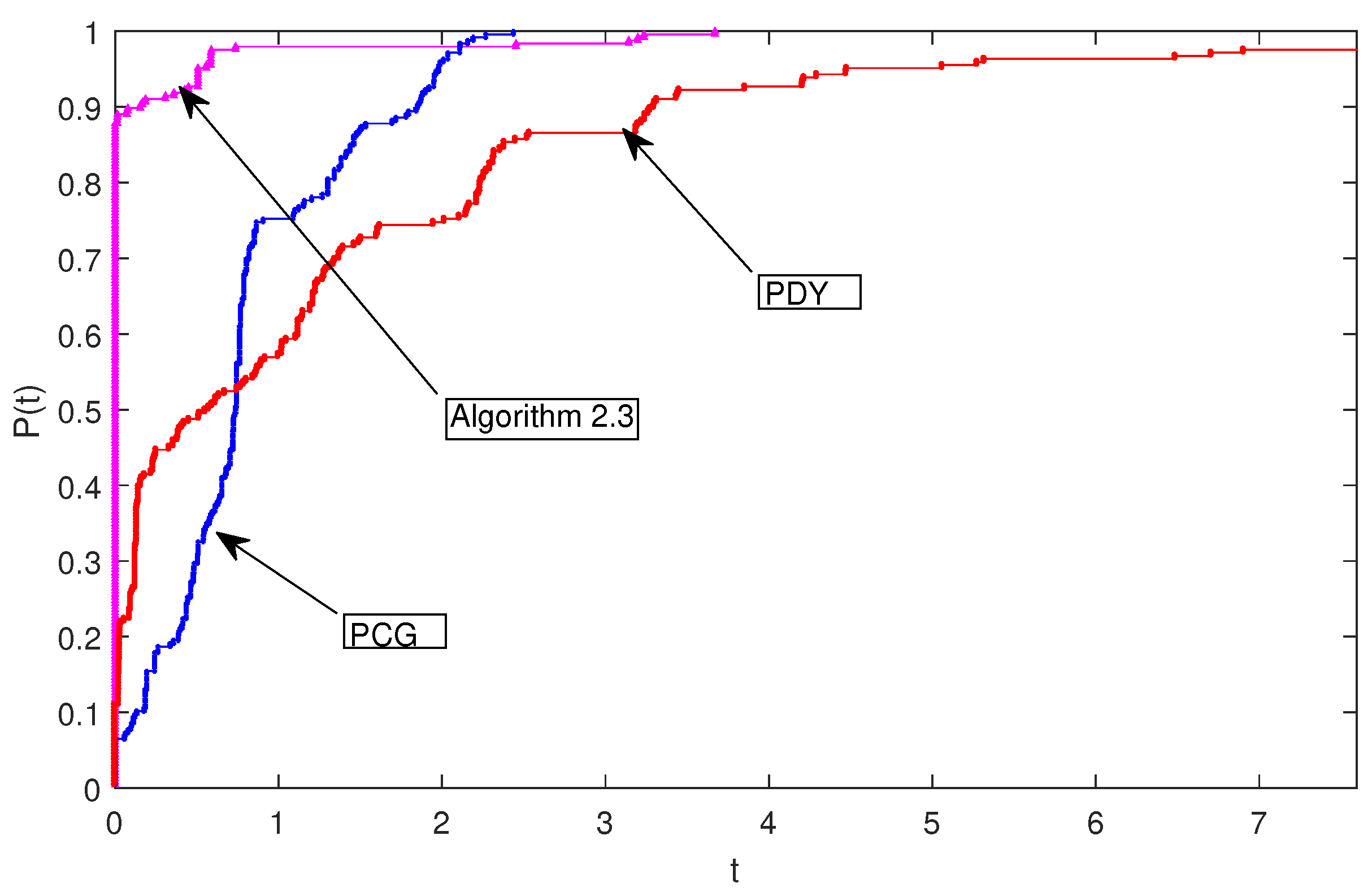
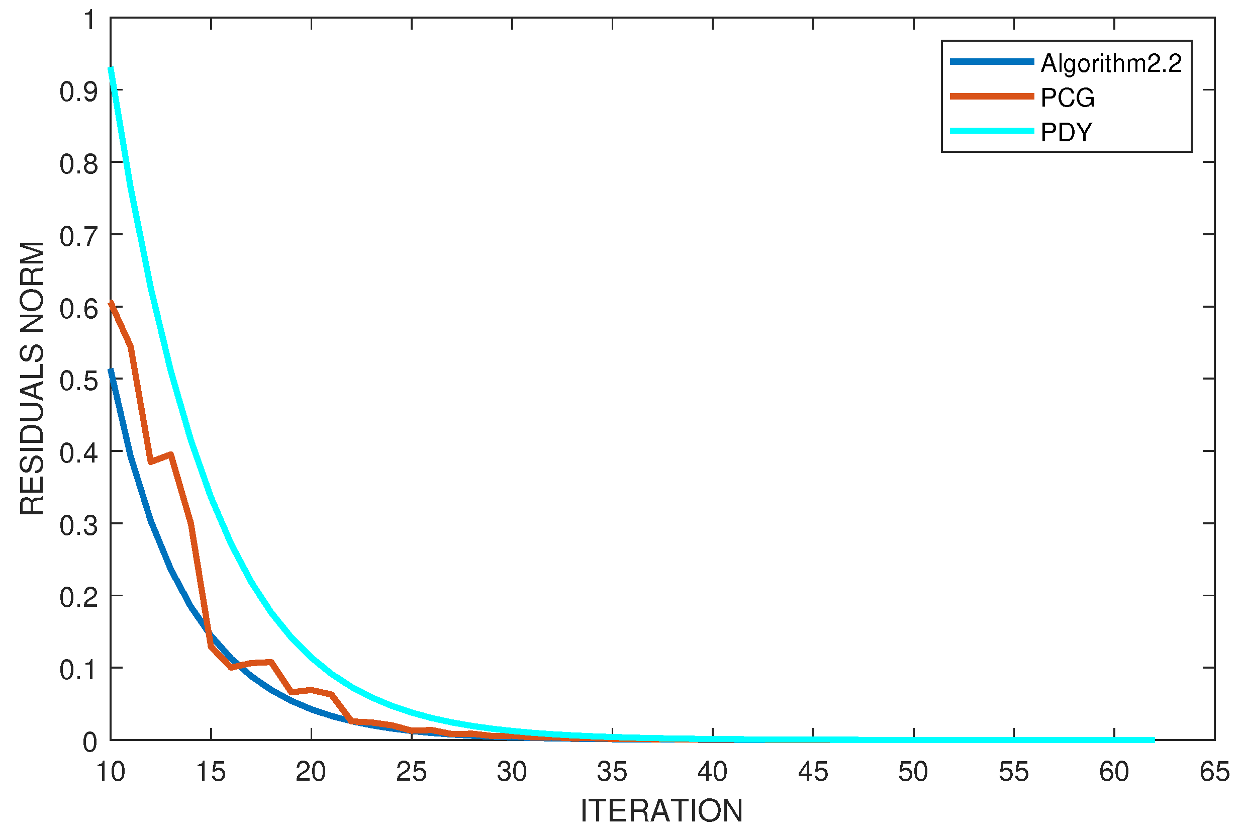
In addition, we employ the performance profile developed in Reference [30] to obtain Figure 1, Figure 2 and Figure 3, which is a helpful process of standardizing the comparison of methods. The measure of the performance profile considered are; number of iterations, CPU time (in seconds) and number of function evaluations. Figure 1 reveals that Algorithm 1 most performs better in terms of number of iterations, as it solves and wins 90 percent of the problems with less number of iterations, while PCG and PDY solves and wins less than 10 percent. In Figure 2, Algorithm 1 performed a little less by solving and winning over 80 percent of the problems with less CPU time as against PCG and PDY with similar performance of less than 10 percent of the problems considered. The translation of Figure 3 is identical to Figure 1. Figure 4 is the plot of the decrease in residual norm against number of iterations on problem 9 with as initial point. It shows the speed of the convergence of each algorithm using the convergence tolerance , it can be observed that Algorithm 1 converges faster than PCG and PDY.
Applications in Compressive Sensing
There are many problems in signal processing and statistical inference involving finding sparse solutions to ill-conditioned linear systems of equations. Among popular approach is minimizing an objective function which contains quadratic () error term and a sparse —regularization term, that is,
where , is an observation, () is a linear operator, is a non-negative parameter, denotes the Euclidean norm of x and is the —norm of x. It is easy to see that problem (24) is a convex unconstrained minimization problem. Due to the fact that if the original signal is sparse or approximately sparse in some orthogonal basis, problem (24) frequently appears in compressive sensing and hence an exact restoration can be produced by solving (24).
Iterative methods for solving (24) have been presented in many papers (see References [5,31,32,33,34,35]). The most popular method among these methods is the gradient based method and the earliest gradient projection method for sparse reconstruction (GPRS) was proposed by Figueiredo et al. [5]. The first step of the GPRS method is to express (24) as a quadratic problem using the following process. Let and splitting it into its positive and negative parts. Then x can be formulated as
where , for all and . By definition of -norm, we have , where . Now (24) can be written as
which is a bound-constrained quadratic program. However, from Reference [5], Equation (25) can be written in standard form as
where , , , .
Clearly, D is a positive semi-definite matrix, which implies that Equation (26) is a convex quadratic problem.
Xiao et al. [19] translated (26) into a linear variable inequality problem which is equivalent to a linear complementarity problem. Furthermore, it was noted that z is a solution of the linear complementarity problem if and only if it is a solution of the nonlinear equation:
The function F is a vector-valued function and the “min” is interpreted as component-wise minimum. It was proved in References [36,37] that is continuous and monotone. Therefore problem (24) can be translated into problem (1) and thus Algorithm 1 (DCG) can be applied to solve it.
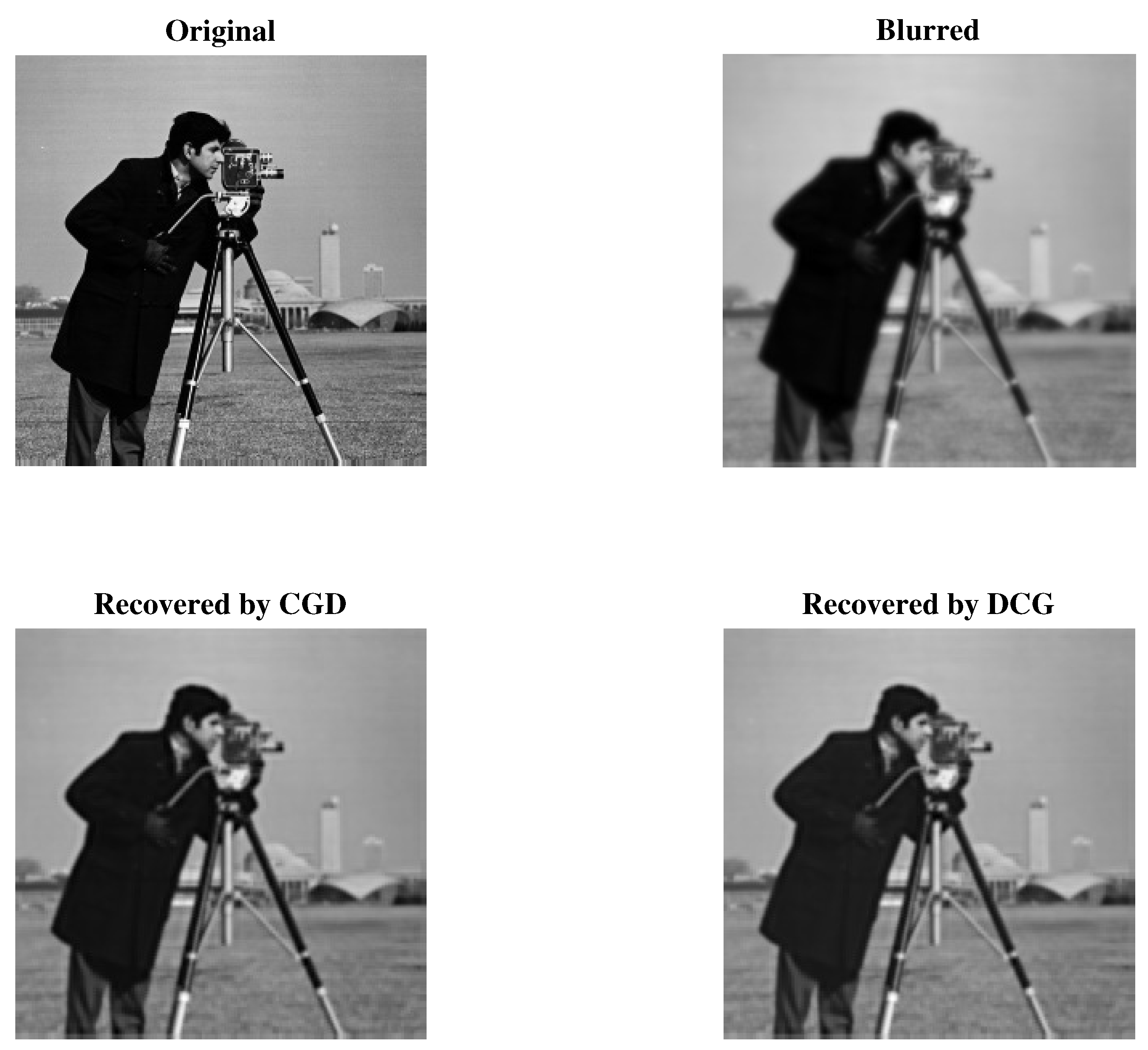
In this experiment, we consider a simple compressive sensing possible situation, where our goal is to restore a blurred image. We use the following well-known gray test images; (P1) Cameraman, (P2) Lena, (P3) House and (P4) Peppers for the experiments. We use 4 different Gaussian blur kernals with standard deviation to compare the robustness of DCG method with CGD method proposed in Reference [19]. CGD method is an extension of the well-known conjugate gradient method for unconstrained optimization CG-DESCENT [20] to solve the -norm regularized problems.
To access the performance of each algorithm tested with respect to metrics that indicate a better quality of restoration, in Table 10 we reported the number of iterations, the objective function (ObjFun) value at the approximate solution, the mean of squared error (MSE) to the original image ,
where is the reconstructed image and the signal-to-noise-ratio (SNR) which is defined as
We also reported the structural similarity (SSIM) index that measure the similarity between the original image and the restored image [38]. The MATLAB implementation of the SSIM index can be obtained at http://www.cns.nyu.edu/~lcv/ssim/.
The original, blurred and restored images by each of the algorithm are given in Figure 5, Figure 6, Figure 7 and Figure 8. The figures demonstrate that both the two tested algorithm can restored the blurred images. It can be observed from Table 10 and Figure 5, Figure 6, Figure 7 and Figure 8 that Algorithm 1 (DCG) compete with the CGD algorithm, therefore, it can be used as an alternative to CGD for restoring blurred image.
4. Conclusions
In this research article, we present a CG method which possesses the sufficient descent property for solving constrained nonlinear monotone equations. The proposed method has the ability to solve non-smooth equations as it does not require matrix storage and Jacobian information of the nonlinear equation under consideration. The sequence of iterates generated converge the solution under appropriate assumptions. Finally, we give some numerical examples to display the efficiency of the proposed method in terms of number of iterations, CPU time and number of function evaluations compared with some related methods for solving convex constrained nonlinear monotone equations and its application in image restoration problems.
Author Contributions
Conceptualization, A.B.A.; methodology, A.B.A.; software, H.M.; validation, P.K. and A.M.A.; formal analysis, P.K. and H.M.; investigation, P.K. and A.M.A.; resources, P.K.; data curation, A.B.A. and H.M.; writing—original draft preparation, A.B.A.; writing—review and editing, H.M.; visualization, A.M.A.; supervision, P.K.; project administration, P.K.; funding acquisition, P.K.
Funding
Petchra Pra Jom Klao Doctoral Scholarship for Ph.D. program of King Mongkut’s University of Technology Thonburi (KMUTT) and Theoretical and Computational Science (TaCS) Center. Moreover, this project was partially supported by the Thailand Research Fund (TRF) and the King Mongkut’s University of Technology Thonburi (KMUTT) under the TRF Research Scholar Award (Grant No. RSA6080047).
Acknowledgments
We thank Associate Professor Jin Kiu Liu for providing us with the access of the CGD-CS MATLAB codes. The authors acknowledge the financial support provided by King Mongkut’s University of Technology Thonburi through the “KMUTT 55th Anniversary Commemorative Fund”. This project is supported by the theoretical and computational science (TaCS) center under computational and applied science for smart research innovation (CLASSIC), Faculty of Science, KMUTT. The first author was supported by the “Petchra Pra Jom Klao Ph.D. Research Scholarship from King Mongkut’s University of Technology Thonburi”.
Conflicts of Interest
The authors declare no conflict of interest.
References
- Gu, B.; Sheng, V.S.; Tay, K.Y.; Romano, W.; Li, S. Incremental support vector learning for ordinal regression. IEEE Trans. Neural Netw. Learn. Syst. 2015, 26, 1403–1416. [Google Scholar] [CrossRef] [PubMed]
- Li, J.; Li, X.; Yang, B.; Sun, X. Segmentation-based image copy-move forgery detection scheme. IEEE Trans. Inf. Forensics Secur. 2015, 10, 507–518. [Google Scholar]
- Wen, X.; Shao, L.; Xue, Y.; Fang, W. A rapid learning algorithm for vehicle classification. Inf. Sci. 2015, 295, 395–406. [Google Scholar] [CrossRef]
- Michael, S.V.; Alfredo, I.N. Newton-type methods with generalized distances for constrained optimization. Optimization 1997, 41, 257–278. [Google Scholar]
- Figueiredo, M.A.T.; Nowak, R.D.; Wright, S.J. Gradient projection for sparse reconstruction: Application to compressed sensing and other inverse problems. IEEE J. Sel. Top. Signal Process. 2007, 1, 586–597. [Google Scholar] [CrossRef]
- Magnanti, T.L.; Perakis, G. Solving variational inequality and fixed point problems by line searches and potential optimization. Math. Program. 2004, 101, 435–461. [Google Scholar] [CrossRef]
- Pan, Z.; Zhang, Y.; Kwong, S. Efficient motion and disparity estimation optimization for low complexity multiview video coding. IEEE Trans. Broadcast. 2015, 61, 166–176. [Google Scholar]
- Xia, Z.; Wang, X.; Sun, X.; Wang, Q. A secure and dynamic multi-keyword ranked search scheme over encrypted cloud data. IEEE Trans. Parallel Distrib. Syst. 2016, 27, 340–352. [Google Scholar] [CrossRef]
- Zheng, Y.; Jeon, B.; Xu, D.; Wu, Q.M.; Zhang, H. Image segmentation by generalized hierarchical fuzzy c-means algorithm. J. Intell. Fuzzy Syst. 2015, 28, 961–973. [Google Scholar]
- Solodov, M.V.; Svaiter, B.F. A globally convergent inexact newton method for systems of monotone equations. In Reformulation: Nonsmooth, Piecewise Smooth, Semismooth and Smoothing Methods; Springer: Dordrecht, The Netherlands, 1998; pp. 355–369. [Google Scholar]
- Mohammad, H.; Abubakar, A.B. A positive spectral gradient-like method for nonlinear monotone equations. Bull. Comput. Appl. Math. 2017, 5, 99–115. [Google Scholar]
- Zhang, L.; Zhou, W. Spectral gradient projection method for solving nonlinear monotone equations. J. Comput. Appl. Math. 2006, 196, 478–484. [Google Scholar] [CrossRef] [Green Version]
- Zhou, W.J.; Li, D.H. A globally convergent BFGS method for nonlinear monotone equations without any merit functions. Math. Comput. 2008, 77, 2231–2240. [Google Scholar] [CrossRef]
- Zhou, W.; Li, D. Limited memory BFGS method for nonlinear monotone equations. J. Comput. Math. 2007, 25, 89–96. [Google Scholar]
- Abubakar, A.B.; Waziria, M.Y. A matrix-free approach for solving systems of nonlinear equations. J. Mod. Methods Numer. Math. 2016, 7, 1–9. [Google Scholar] [CrossRef]
- Abubakar, A.B.; Kumam, P. An improved three-term derivative-free method for solving nonlinear equations. Comput. Appl. Math. 2018, 37, 6760–6773. [Google Scholar] [CrossRef]
- Abubakar, A.B.; Kumam, P.; Awwal, A.M. A descent dai-liao projection method for convex constrained nonlinear monotone equations with applications. Thai J. Math. 2018, 17, 128–152. [Google Scholar]
- Wang, C.; Wang, Y.; Xu, C. A projection method for a system of nonlinear monotone equations with convex constraints. Math. Methods Oper. Res. 2007, 66, 33–46. [Google Scholar] [CrossRef]
- Xiao, Y.; Zhu, H. A conjugate gradient method to solve convex constrained monotone equations with applications in compressive sensing. J. Math. Anal. Appl. 2013, 405, 310–319. [Google Scholar] [CrossRef]
- Hager, W.; Zhang, H. A new conjugate gradient method with guaranteed descent and an efficient line search. SIAM J. Optim. 2005, 16, 170–192. [Google Scholar] [CrossRef]
- Liu, S.-Y.; Huang, Y.-Y.; Jiao, H.-W. Sufficient descent conjugate gradient methods for solving convex constrained nonlinear monotone equations. Abstr. Appl. Anal. 2014, 2014, 305643. [Google Scholar] [CrossRef]
- Liu, J.K.; Li, S.J. A projection method for convex constrained monotone nonlinear equations with applications. Comput. Math. Appl. 2015, 70, 2442–2453. [Google Scholar] [CrossRef]
- Ding, Y.; Xiao, Y.; Li, J. A class of conjugate gradient methods for convex constrained monotone equations. Optimization 2017, 66, 2309–2328. [Google Scholar] [CrossRef]
- Liu, J.; Feng, Y. A derivative-free iterative method for nonlinear monotone equations with convex constraints. Numer. Algorithms 2018, 1–18. [Google Scholar] [CrossRef]
- Muhammed, A.A.; Kumam, P.; Abubakar, A.B.; Wakili, A.; Pakkaranang, N. A new hybrid spectral gradient projection method for monotone system of nonlinear equations with convex constraints. Thai J. Math. 2018, 16, 125–147. [Google Scholar]
- La Cruz, W.; Martínez, J.; Raydan, M. Spectral residual method without gradient information for solving large-scale nonlinear systems of equations. Math. Comput. 2006, 75, 1429–1448. [Google Scholar] [CrossRef]
- Bing, Y.; Lin, G. An efficient implementation of Merrill’s method for sparse or partially separable systems of nonlinear equations. SIAM J. Optim. 1991, 1, 206–221. [Google Scholar] [CrossRef]
- Yu, Z.; Lin, J.; Sun, J.; Xiao, Y.H.; Liu, L.Y.; Li, Z.H. Spectral gradient projection method for monotone nonlinear equations with convex constraints. Appl. Numer. Math. 2009, 59, 2416–2423. [Google Scholar] [CrossRef]
- Yamashita, N.; Fukushima, M. Modified Newton methods for solving a semismooth reformulation of monotone complementarity problems. Math. Program. 1997, 76, 469–491. [Google Scholar] [CrossRef]
- Dolan, E.D.; Moré, J.J. Benchmarking optimization software with performance profiles. Math. Program. 2002, 91, 201–213. [Google Scholar] [CrossRef]
- Figueiredo, M.A.T.; Nowak, R.D. An EM algorithm for wavelet-based image restoration. IEEE Trans. Image Process. 2003, 12, 906–916. [Google Scholar] [CrossRef] [Green Version]
- Hale, E.T.; Yin, W.; Zhang, Y. A Fixed-Point Continuation Method for ℓ1-Regularized Minimization with Applications to Compressed Sensing; CAAM TR07-07; Rice University: Houston, TX, USA, 2007; pp. 43–44. [Google Scholar]
- Beck, A.; Teboulle, M. A fast iterative shrinkage-thresholding algorithm for linear inverse problems. SIAM J. Imaging Sci. 2009, 2, 183–202. [Google Scholar] [CrossRef]
- Van Den Berg, E.; Friedlander, M.P. Probing the pareto frontier for basis pursuit solutions. SIAM J. Sci. Comput. 2008, 31, 890–912. [Google Scholar] [CrossRef]
- Birgin, E.G.; Martínez, J.M.; Raydan, M. Nonmonotone spectral projected gradient methods on convex sets. SIAM J. Optim. 2000, 10, 1196–1211. [Google Scholar] [CrossRef]
- Xiao, Y.; Wang, Q.; Hu, Q. Non-smooth equations based method for ℓ1-norm problems with applications to compressed sensing. Nonlinear Anal. Theory Methods Appl. 2011, 74, 3570–3577. [Google Scholar] [CrossRef]
- Pang, J.-S. Inexact Newton methods for the nonlinear complementarity problem. Math. Program. 1986, 36, 54–71. [Google Scholar] [CrossRef]
- Wang, Z.; Bovik, A.C.; Sheikh, H.R.; Simoncelli, E.P. Image quality assessment: From error visibility to structural similarity. IEEE Trans. Image Process. 2004, 13, 600–612. [Google Scholar] [CrossRef]
Figure 1.
Performance profiles for the number of iterations.

Figure 2.
Performance profiles for the CPU time (in seconds).

Figure 3.
Performance profiles for the number of function evaluations.

Figure 4.
Convergence histories of Algorithm 1, PCG and PDY on Problem 9.

Figure 5.
The original image (top left), the blurred image (top right), the restored image by CGD (bottom left) with SNR = 20.05, SSIM = 0.83 and by DCG (bottom right) with SNR = 20.12, SSIM = 0.83.
Figure 5.
The original image (top left), the blurred image (top right), the restored image by CGD (bottom left) with SNR = 20.05, SSIM = 0.83 and by DCG (bottom right) with SNR = 20.12, SSIM = 0.83.

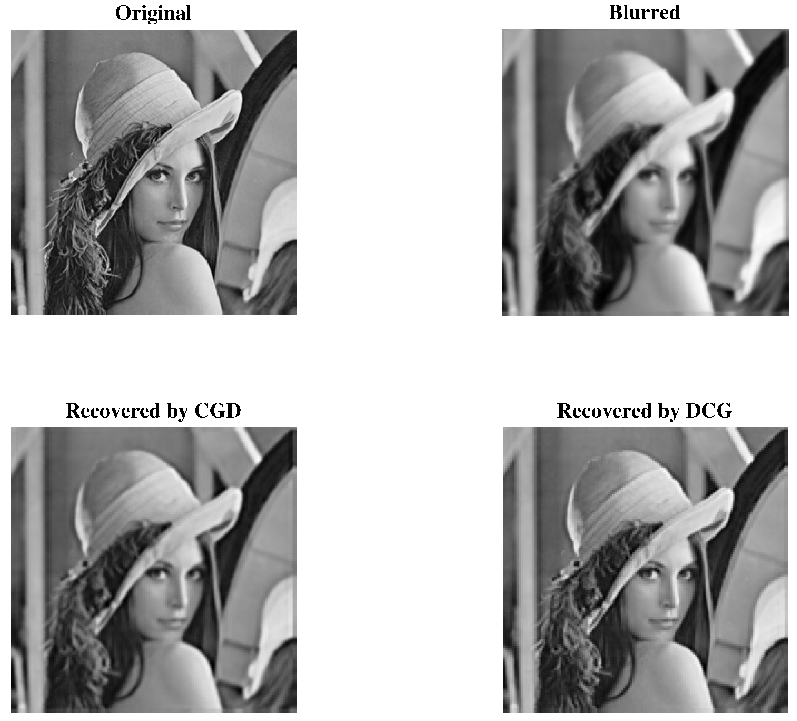
Figure 6.
The original image (top left), the blurred image (top right), the restored image by CGD (bottom left) with SNR = 22.93, SSIM = 0.87 and by DCG (bottom right) with SNR = 24.36, SSIM = 0.90.
Figure 6.
The original image (top left), the blurred image (top right), the restored image by CGD (bottom left) with SNR = 22.93, SSIM = 0.87 and by DCG (bottom right) with SNR = 24.36, SSIM = 0.90.

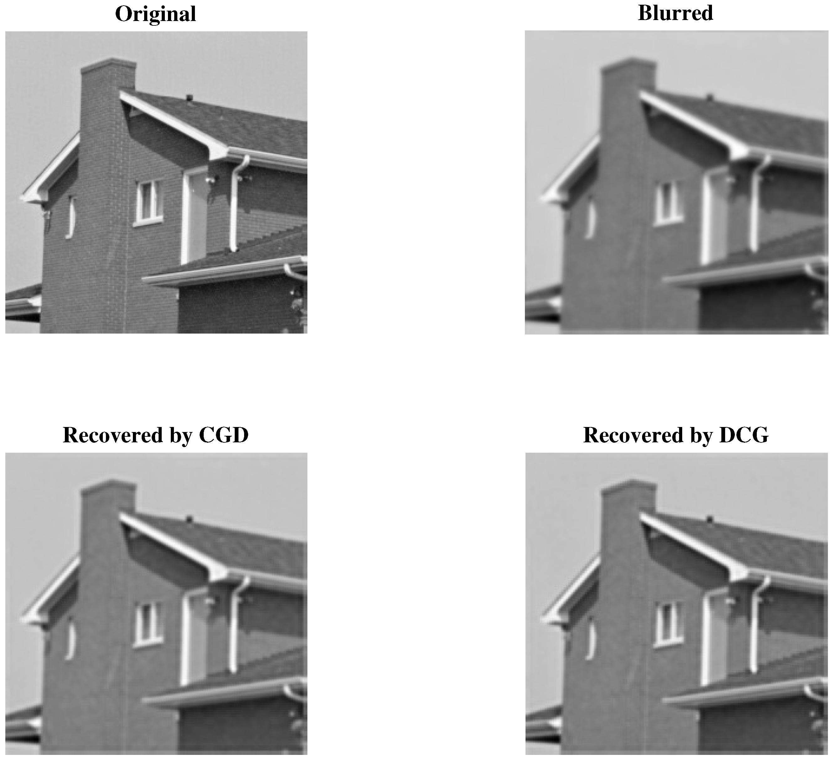
Figure 7.
The original image (top left), the blurred image (top right), the restored image by CGD (bottom left) with SNR = 25.65, SSIM = 0.86 and by DCG (bottom right) with SNR = 26.37, SSIM = 0.87.
Figure 7.
The original image (top left), the blurred image (top right), the restored image by CGD (bottom left) with SNR = 25.65, SSIM = 0.86 and by DCG (bottom right) with SNR = 26.37, SSIM = 0.87.

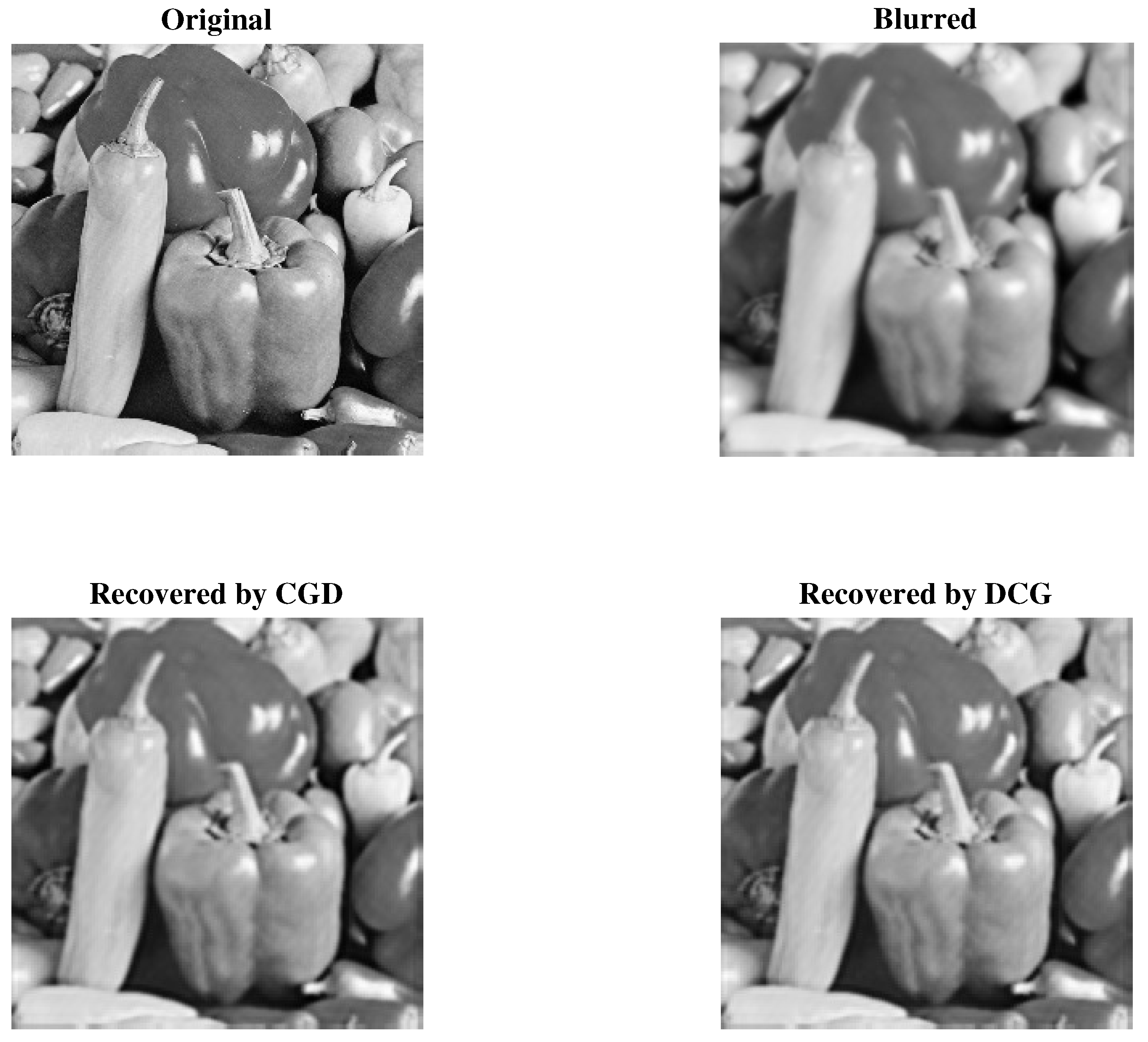
Figure 8.
The original image (top left), the blurred image (top right), the restored image by CGD (bottom left) with SNR = 21.50, SSIM = 0.84 and by DCG (bottom right) with SNR = 21.81, SSIM = 0.85.
Figure 8.
The original image (top left), the blurred image (top right), the restored image by CGD (bottom left) with SNR = 21.50, SSIM = 0.84 and by DCG (bottom right) with SNR = 21.81, SSIM = 0.85.


Table 1.
Numerical Results for Algorithm 1 (DCG), PCG and PDY for Problem 1 with given initial points and dimensions.
Table 1.
Numerical Results for Algorithm 1 (DCG), PCG and PDY for Problem 1 with given initial points and dimensions.
| Algorithm 1 | PCG | PDY | |||||||||||
|---|---|---|---|---|---|---|---|---|---|---|---|---|---|
| DIMENSION | INITIAL POINT | ITER | FVAL | TIME | NORM | ITER | FVAL | TIME | NORM | ITER | FVAL | TIME | NORM |
| 1000 | 11 | 49 | 0.025557 | 8.88 | 18 | 73 | 0.019295 | 5.72 | 12 | 49 | 0.16248 | 9.18 | |
| 12 | 53 | 0.014164 | 4.78 | 18 | 73 | 0.011648 | 9.82 | 13 | 53 | 0.03780 | 6.35 | ||
| 12 | 53 | 0.008524 | 8.75 | 19 | 77 | 0.011197 | 7.1 | 14 | 57 | 0.01550 | 5.59 | ||
| 13 | 57 | 0.011333 | 6.68 | 18 | 73 | 0.022197 | 8.27 | 15 | 61 | 0.01746 | 4.07 | ||
| 13 | 57 | 0.014202 | 6.09 | 63 | 254 | 0.046072 | 9.58 | 14 | 57 | 0.02193 | 9.91 | ||
| 13 | 57 | 0.011045 | 8.14 | 61 | 246 | 0.031608 | 9.15 | 40 | 162 | 0.03472 | 9.70 | ||
| 5000 | 12 | 53 | 0.024311 | 5.82 | 18 | 73 | 0.11431 | 7.42 | 13 | 53 | 0.03158 | 6.87 | |
| 13 | 57 | 0.027361 | 3.13 | 19 | 77 | 0.03997 | 6.53 | 14 | 57 | 0.04270 | 4.62 | ||
| 13 | 57 | 0.02541 | 5.73 | 20 | 81 | 0.056159 | 5.2 | 15 | 61 | 0.05433 | 4.18 | ||
| 14 | 61 | 0.032038 | 4.38 | 19 | 77 | 0.038381 | 8.1 | 15 | 61 | 0.04357 | 9.08 | ||
| 14 | 61 | 0.039044 | 3.98 | 62 | 250 | 0.15836 | 9.53 | 15 | 61 | 0.08960 | 7.30 | ||
| 14 | 61 | 0.027231 | 5.33 | 60 | 242 | 0.13276 | 9.1 | 39 | 158 | 0.11284 | 9.86 | ||
| 10,000 | 12 | 53 | 0.05434 | 8.23 | 18 | 73 | 0.073207 | 9.5 | 13 | 53 | 0.06371 | 9.70 | |
| 13 | 57 | 0.045664 | 4.43 | 19 | 77 | 0.090771 | 8.15 | 14 | 57 | 0.06336 | 6.53 | ||
| 13 | 57 | 0.041922 | 8.09 | 20 | 81 | 0.070859 | 6.74 | 15 | 61 | 0.06414 | 5.90 | ||
| 14 | 61 | 0.047641 | 6.2 | 20 | 81 | 0.087357 | 5.11 | 16 | 65 | 0.07920 | 4.28 | ||
| 14 | 61 | 0.045734 | 5.62 | 62 | 250 | 0.24646 | 8.87 | 39 | 158 | 0.22101 | 7.97 | ||
| 14 | 61 | 0.057104 | 7.54 | 59 | 238 | 0.19949 | 9.96 | 87 | 351 | 0.36237 | 9.93 | ||
| 50,000 | 13 | 57 | 0.16384 | 5.41 | 19 | 77 | 0.25487 | 8.8 | 14 | 57 | 0.27607 | 7.12 | |
| 13 | 57 | 0.18633 | 9.9 | 20 | 81 | 0.32689 | 7.39 | 15 | 61 | 0.26220 | 4.91 | ||
| 14 | 61 | 0.20801 | 5.32 | 21 | 85 | 0.33649 | 6.31 | 16 | 65 | 0.28260 | 4.37 | ||
| 15 | 65 | 0.1946 | 4.08 | 21 | 85 | 0.32779 | 5.1 | 38 | 154 | 0.60650 | 7.54 | ||
| 15 | 65 | 0.19799 | 3.69 | 61 | 246 | 0.82615 | 8.85 | 177 | 712 | 2.52330 | 9.44 | ||
| 15 | 65 | 0.22418 | 4.95 | 59 | 238 | 0.79992 | 8.5 | 361 | 1449 | 5.97950 | 9.74 | ||
| 100,000 | 13 | 57 | 0.32291 | 7.65 | 20 | 81 | 0.53846 | 5.52 | 15 | 61 | 0.39342 | 3.39 | |
| 14 | 61 | 0.33329 | 4.12 | 21 | 85 | 0.61533 | 4.62 | 15 | 61 | 0.42154 | 6.94 | ||
| 14 | 61 | 0.37048 | 7.52 | 21 | 85 | 0.53638 | 8.78 | 16 | 65 | 0.45851 | 6.18 | ||
| 15 | 65 | 0.36058 | 5.76 | 21 | 85 | 0.62002 | 7.21 | 175 | 704 | 4.36100 | 9.47 | ||
| 15 | 65 | 0.34975 | 5.22 | 60 | 242 | 1.4564 | 9.73 | 176 | 708 | 4.29180 | 9.91 | ||
| 15 | 65 | 0.3621 | 7.01 | 58 | 234 | 1.4155 | 9.42 | 360 | 1445 | 9.71190 | 9.99 | ||
Table 2.
Numerical Results for Algorithm 1 (DCG), PCG and PDY for Problem 2 with given initial points and dimensions.
Table 2.
Numerical Results for Algorithm 1 (DCG), PCG and PDY for Problem 2 with given initial points and dimensions.
| Algorithm 1 | PCG | PDY | |||||||||||
|---|---|---|---|---|---|---|---|---|---|---|---|---|---|
| DIMENSION | INITIAL POINT | ITER | FVAL | TIME | NORM | ITER | FVAL | TIME | NORM | ITER | FVAL | TIME | NORM |
| 1000 | 9 | 38 | 3.1744 | 5.84 | 15 | 59 | 0.049899 | 8.59 | 10 | 39 | 0.01053 | 6.96 | |
| 10 | 42 | 0.014633 | 6.25 | 11 | 42 | 0.015089 | 9.07 | 11 | 43 | 0.00937 | 9.23 | ||
| 9 | 38 | 0.017067 | 7.4 | 17 | 66 | 0.016935 | 6.44 | 13 | 51 | 0.01111 | 6.26 | ||
| 7 | 30 | 0.006392 | 6.53 | 18 | 69 | 0.01436 | 6 | 14 | 55 | 0.02154 | 9.46 | ||
| 11 | 46 | 0.011954 | 3.47 | 13 | 48 | 0.00907 | 7.58 | 15 | 59 | 0.01850 | 4.60 | ||
| 12 | 50 | 0.68666 | 6.74 | 18 | 68 | 0.01352 | 5.4 | 15 | 59 | 0.01938 | 7.71 | ||
| 5000 | 10 | 42 | 0.11241 | 3.53 | 16 | 63 | 0.041151 | 9.35 | 11 | 43 | 0.03528 | 4.86 | |
| 11 | 46 | 0.028723 | 3.81 | 12 | 46 | 0.028706 | 8.8 | 12 | 47 | 0.04032 | 6.89 | ||
| 10 | 42 | 0.029367 | 4.3 | 18 | 70 | 0.047532 | 6.98 | 14 | 55 | 0.04889 | 4.61 | ||
| 13 | 54 | 0.036231 | 3.67 | 19 | 73 | 0.052164 | 6.45 | 15 | 59 | 0.04826 | 6.96 | ||
| 11 | 46 | 0.04963 | 7.21 | 14 | 52 | 0.040529 | 6.71 | 16 | 63 | 0.05969 | 3.37 | ||
| 13 | 54 | 0.054971 | 4.05 | 19 | 72 | 0.12303 | 5.71 | 16 | 63 | 0.06253 | 5.64 | ||
| 10,000 | 10 | 42 | 0.049614 | 4.98 | 17 | 67 | 0.074779 | 6.6 | 11 | 43 | 0.06732 | 6.85 | |
| 11 | 46 | 0.061595 | 5.36 | 13 | 50 | 0.08308 | 6.11 | 12 | 47 | 0.12232 | 9.72 | ||
| 10 | 42 | 0.054587 | 6.02 | 18 | 70 | 0.085554 | 9.83 | 14 | 55 | 0.08288 | 6.51 | ||
| 13 | 54 | 0.073333 | 5.16 | 19 | 73 | 0.10579 | 9.07 | 15 | 59 | 0.08413 | 9.82 | ||
| 12 | 50 | 0.06306 | 2.83 | 14 | 52 | 0.074982 | 9.18 | 16 | 63 | 0.09589 | 4.75 | ||
| 13 | 54 | 0.062259 | 5.69 | 19 | 72 | 0.099167 | 8.02 | 16 | 64 | 0.11499 | 8.55 | ||
| 50,000 | 11 | 46 | 0.20703 | 3.1 | 18 | 71 | 0.39473 | 7.37 | 12 | 47 | 0.27826 | 5.23 | |
| 12 | 50 | 0.23251 | 3.35 | 14 | 54 | 0.27346 | 6.74 | 13 | 51 | 0.29642 | 7.11 | ||
| 11 | 46 | 0.21338 | 3.73 | 20 | 78 | 0.37249 | 5.5 | 15 | 59 | 0.35602 | 4.82 | ||
| 14 | 58 | 0.3232 | 3.22 | 21 | 81 | 0.37591 | 5.07 | 35 | 141 | 0.69470 | 6.69 | ||
| 12 | 50 | 0.22703 | 6.27 | 16 | 60 | 0.26339 | 5.02 | 35 | 141 | 0.68488 | 9.12 | ||
| 14 | 58 | 0.25979 | 3.54 | 20 | 76 | 0.33814 | 8.93 | 35 | 141 | 0.70973 | 9.91 | ||
| 100,000 | 11 | 46 | 0.55511 | 4.38 | 19 | 75 | 0.65494 | 5.22 | 12 | 47 | 0.44541 | 7.39 | |
| 12 | 50 | 0.54694 | 4.73 | 14 | 54 | 0.4944 | 9.52 | 14 | 55 | 0.53299 | 3.39 | ||
| 11 | 46 | 0.40922 | 5.27 | 20 | 78 | 0.78319 | 7.78 | 15 | 60 | 0.58603 | 8.71 | ||
| 14 | 58 | 0.62049 | 4.55 | 21 | 81 | 0.76051 | 7.17 | 72 | 290 | 2.70630 | 8.31 | ||
| 12 | 50 | 0.47039 | 8.86 | 16 | 60 | 0.58545 | 7.07 | 72 | 290 | 2.72220 | 8.68 | ||
| 14 | 58 | 0.71174 | 5.01 | 21 | 80 | 0.77051 | 6.32 | 72 | 290 | 2.75850 | 8.96 | ||
Table 3.
Numerical Results for Algorithm 1 (DCG), PCG and PDY for Problem 3 with given initial points and dimensions.
Table 3.
Numerical Results for Algorithm 1 (DCG), PCG and PDY for Problem 3 with given initial points and dimensions.
| Algorithm 1 (DCG) | PCG | PDY | |||||||||||
|---|---|---|---|---|---|---|---|---|---|---|---|---|---|
| DIMENSION | INITIAL POINT | ITER | FVAL | TIME | NORM | ITER | FVAL | TIME | NORM | ITER | FVAL | TIME | NORM |
| 1000 | 10 | 43 | 0.75322 | 9.9 | 19 | 76 | 0.55752 | 5.62 | 12 | 48 | 0.01255 | 4.45 | |
| 11 | 47 | 0.006933 | 5.46 | 20 | 80 | 0.010936 | 5.58 | 12 | 48 | 0.01311 | 9.02 | ||
| 12 | 51 | 0.00676 | 3.48 | 21 | 84 | 0.011048 | 6.58 | 13 | 52 | 0.01486 | 8.34 | ||
| 12 | 51 | 0.009664 | 4.41 | 22 | 88 | 0.011058 | 5.67 | 14 | 56 | 0.01698 | 8.04 | ||
| 11 | 47 | 0.010487 | 9.06 | 22 | 88 | 0.012198 | 5.64 | 14 | 56 | 0.01551 | 9.72 | ||
| 13 | 55 | 0.012702 | 3.15 | 21 | 84 | 0.018231 | 8.36 | 14 | 56 | 0.01534 | 9.42 | ||
| 5000 | 11 | 47 | 0.019458 | 6.19 | 20 | 80 | 0.040808 | 6.29 | 12 | 48 | 0.03660 | 9.94 | |
| 12 | 51 | 0.021562 | 3.42 | 21 | 84 | 0.06688 | 6.25 | 13 | 52 | 0.03616 | 6.85 | ||
| 12 | 51 | 0.024274 | 7.79 | 22 | 88 | 0.04144 | 7.37 | 14 | 56 | 0.04594 | 6.14 | ||
| 12 | 51 | 0.026771 | 9.86 | 23 | 92 | 0.052214 | 6.35 | 15 | 60 | 0.04342 | 6.01 | ||
| 12 | 51 | 0.026814 | 5.67 | 23 | 92 | 0.041444 | 6.31 | 15 | 60 | 0.04296 | 7.25 | ||
| 13 | 55 | 0.023903 | 7.03 | 22 | 88 | 0.040135 | 9.37 | 32 | 129 | 0.10081 | 8.85 | ||
| 10,000 | 11 | 47 | 0.044134 | 8.75 | 20 | 80 | 0.064312 | 8.9 | 13 | 52 | 0.06192 | 4.77 | |
| 12 | 51 | 0.051947 | 4.83 | 21 | 84 | 0.088102 | 8.84 | 13 | 52 | 0.06442 | 9.68 | ||
| 13 | 55 | 0.057291 | 3.08 | 23 | 92 | 0.07296 | 5.22 | 14 | 56 | 0.09499 | 8.69 | ||
| 13 | 55 | 0.055134 | 3.9 | 23 | 92 | 0.075265 | 8.99 | 15 | 60 | 0.07696 | 8.5 | ||
| 12 | 51 | 0.047551 | 8.02 | 23 | 92 | 0.073937 | 8.93 | 33 | 133 | 0.18625 | 6.45 | ||
| 13 | 55 | 0.055069 | 9.95 | 23 | 92 | 0.099888 | 6.64 | 33 | 133 | 0.15548 | 7.51 | ||
| 50,000 | 12 | 51 | 0.19938 | 5.47 | 21 | 84 | 0.27031 | 9.97 | 14 | 56 | 0.23642 | 3.51 | |
| 13 | 55 | 0.22499 | 3.02 | 22 | 88 | 0.2657 | 9.9 | 14 | 56 | 0.24813 | 7.12 | ||
| 13 | 55 | 0.19396 | 6.89 | 24 | 96 | 0.3246 | 5.85 | 15 | 60 | 0.27049 | 6.53 | ||
| 13 | 55 | 0.20259 | 8.72 | 25 | 100 | 0.32373 | 5.04 | 34 | 137 | 0.54545 | 7.13 | ||
| 13 | 55 | 0.19452 | 5.01 | 25 | 100 | 0.33764 | 5.01 | 68 | 274 | 1.02330 | 9.99 | ||
| 14 | 59 | 0.22015 | 6.22 | 24 | 96 | 0.33687 | 7.44 | 69 | 278 | 1.03810 | 8.05 | ||
| 100,000 | 12 | 51 | 0.39983 | 7.74 | 22 | 88 | 0.63809 | 7.06 | 14 | 56 | 0.45475 | 4.96 | |
| 13 | 55 | 0.32765 | 4.28 | 23 | 92 | 0.63458 | 7.02 | 15 | 60 | 0.49018 | 3.39 | ||
| 13 | 55 | 0.30133 | 9.75 | 24 | 96 | 0.71422 | 8.27 | 15 | 60 | 0.49016 | 9.24 | ||
| 14 | 59 | 0.42865 | 3.45 | 25 | 100 | 0.73524 | 7.13 | 139 | 559 | 4.03110 | 9.01 | ||
| 13 | 55 | 0.34512 | 7.09 | 25 | 100 | 0.70625 | 7.09 | 70 | 282 | 2.07100 | 8.54 | ||
| 14 | 59 | 0.40387 | 8.8 | 25 | 100 | 0.76777 | 5.27 | 139 | 559 | 4.02440 | 9.38 | ||
Table 4.
Numerical Results for Algorithm 1 (DCG), PCG and PDY for Problem 4 with given initial points and dimensions.
Table 4.
Numerical Results for Algorithm 1 (DCG), PCG and PDY for Problem 4 with given initial points and dimensions.
| Algorithm 1 | PCG | PDY | |||||||||||
|---|---|---|---|---|---|---|---|---|---|---|---|---|---|
| DIMENSION | INITIAL POINT | ITER | FVAL | TIME | NORM | ITER | FVAL | TIME | NORM | ITER | FVAL | TIME | NORM |
| 1000 | 10 | 43 | 0.15461 | 8.33 | 18 | 72 | 0.11853 | 9.93 | 12 | 48 | 0.00989 | 4.60 | |
| 11 | 47 | 0.006276 | 3.84 | 19 | 76 | 0.014318 | 8.75 | 12 | 48 | 0.00966 | 9.57 | ||
| 11 | 47 | 0.009859 | 3.91 | 20 | 80 | 0.0093776 | 7.15 | 13 | 52 | 0.00887 | 8.49 | ||
| 11 | 47 | 0.007976 | 5.21 | 47 | 189 | 0.023321 | 7.83 | 12 | 48 | 0.01207 | 5.83 | ||
| 12 | 51 | 0.008382 | 4.09 | 46 | 185 | 0.047105 | 9.76 | 29 | 117 | 0.05371 | 9.43 | ||
| 12 | 51 | 0.008645 | 3.32 | 41 | 165 | 0.027719 | 8.77 | 29 | 117 | 0.02396 | 6.65 | ||
| 5000 | 11 | 47 | 0.022024 | 5.21 | 20 | 80 | 0.029445 | 5.57 | 13 | 52 | 0.02503 | 3.49 | |
| 11 | 47 | 0.020587 | 8.59 | 20 | 80 | 0.033115 | 9.8 | 13 | 52 | 0.02626 | 7.24 | ||
| 11 | 47 | 0.023714 | 8.75 | 21 | 84 | 0.033318 | 8.01 | 14 | 56 | 0.03349 | 6.29 | ||
| 12 | 51 | 0.024728 | 3.26 | 49 | 197 | 0.071715 | 9.46 | 13 | 52 | 0.02258 | 4.25 | ||
| 12 | 51 | 0.031015 | 9.14 | 49 | 197 | 0.068565 | 8.68 | 31 | 125 | 0.05471 | 7.59 | ||
| 12 | 51 | 0.030012 | 7.43 | 44 | 177 | 0.070862 | 7.79 | 63 | 254 | 0.10064 | 8.54 | ||
| 10,000 | 11 | 47 | 0.041476 | 7.37 | 20 | 80 | 0.043013 | 7.88 | 13 | 52 | 0.03761 | 4.93 | |
| 12 | 51 | 0.047866 | 3.4 | 21 | 84 | 0.051685 | 6.94 | 14 | 56 | 0.04100 | 3.37 | ||
| 12 | 51 | 0.042607 | 3.46 | 22 | 88 | 0.050422 | 5.67 | 14 | 56 | 0.03919 | 8.90 | ||
| 12 | 51 | 0.036406 | 4.61 | 50 | 201 | 0.17563 | 9.84 | 32 | 129 | 0.09613 | 6.02 | ||
| 13 | 55 | 0.041374 | 3.61 | 50 | 201 | 0.20035 | 9.03 | 32 | 129 | 0.09177 | 6.44 | ||
| 13 | 55 | 0.039847 | 2.94 | 45 | 181 | 0.12214 | 8.11 | 64 | 258 | 0.20791 | 9.39 | ||
| 50,000 | 12 | 51 | 0.13928 | 4.61 | 21 | 84 | 0.27145 | 8.83 | 14 | 56 | 0.17193 | 3.63 | |
| 12 | 51 | 0.18031 | 7.6 | 22 | 88 | 0.23149 | 7.78 | 14 | 56 | 0.15237 | 7.54 | ||
| 12 | 51 | 0.12526 | 7.74 | 23 | 92 | 0.28789 | 6.36 | 15 | 60 | 0.16549 | 6.66 | ||
| 13 | 55 | 0.14322 | 2.88 | 53 | 213 | 0.61624 | 8.75 | 67 | 270 | 0.76283 | 7.81 | ||
| 13 | 55 | 0.17904 | 8.08 | 53 | 213 | 0.7119 | 8.02 | 67 | 270 | 0.76157 | 8.80 | ||
| 13 | 55 | 0.13635 | 6.57 | 47 | 189 | 0.48192 | 9.8 | 269 | 1080 | 2.92510 | 9.41 | ||
| 100,000 | 12 | 51 | 0.24293 | 6.52 | 22 | 88 | 0.60822 | 6.25 | 14 | 56 | 0.30229 | 5.13 | |
| 13 | 55 | 0.27433 | 3.01 | 23 | 92 | 0.52965 | 5.51 | 15 | 60 | 0.31648 | 3.59 | ||
| 13 | 55 | 0.2714 | 3.06 | 23 | 92 | 0.57064 | 8.99 | 32 | 129 | 0.72838 | 9.99 | ||
| 13 | 55 | 0.26819 | 4.08 | 54 | 217 | 1.1805 | 9.1 | 135 | 543 | 2.86780 | 9.73 | ||
| 14 | 59 | 0.31696 | 3.2 | 54 | 217 | 1.107 | 8.34 | 272 | 1092 | 5.74140 | 9.91 | ||
| 13 | 55 | 0.2698 | 9.29 | 49 | 197 | 1.0617 | 7.49 | 548 | 2197 | 11.44130 | 9.87 | ||
Table 5.
Numerical Results for Algorithm 1 (DCG), PCG and PDY for Problem 5 with given initial points and dimensions.
Table 5.
Numerical Results for Algorithm 1 (DCG), PCG and PDY for Problem 5 with given initial points and dimensions.
| Algorithm 1 | PCG | PDY | |||||||||||
|---|---|---|---|---|---|---|---|---|---|---|---|---|---|
| DIMENSION | INITIAL POINT | ITER | FVAL | TIME | NORM | ITER | FVAL | TIME | NORM | ITER | FVAL | TIME | NORM |
| 1000 | 19 | 78 | 0.71709 | 8.63 | 22 | 83 | 0.099338 | 7.48 | 16 | 63 | 0.07575 | 6.03 | |
| 21 | 86 | 0.017127 | 7.65 | 23 | 88 | 0.016014 | 7.31 | 16 | 63 | 0.01470 | 5.42 | ||
| 23 | 95 | 0.013909 | 7.23 | 23 | 90 | 0.016328 | 9.31 | 33 | 132 | 0.02208 | 6.75 | ||
| 22 | 92 | 0.0165 | 8.64 | 49 | 197 | 0.030124 | 8.45 | 30 | 121 | 0.01835 | 8.39 | ||
| 35 | 145 | 0.024702 | 8.26 | 53 | 213 | 0.039321 | 8.38 | 32 | 129 | 0.02700 | 8.47 | ||
| 43 | 182 | 0.027471 | 8.7 | 46 | 185 | 0.033627 | 8.8 | 30 | 121 | 0.01712 | 6.95 | ||
| 5000 | 146 | 592 | 0.23803 | 9.45 | 24 | 91 | 0.060158 | 6.36 | 17 | 67 | 0.04394 | 5.64 | |
| 21 | 86 | 0.04337 | 9.46 | 25 | 95 | 0.060385 | 6.24 | 17 | 67 | 0.04635 | 5.07 | ||
| 24 | 99 | 0.054619 | 8.27 | 25 | 98 | 0.040015 | 5.86 | 35 | 140 | 0.08311 | 9.74 | ||
| 24 | 100 | 0.066424 | 6.66 | 53 | 213 | 0.098097 | 9.11 | 33 | 133 | 0.08075 | 6.02 | ||
| 38 | 157 | 0.071222 | 9.28 | 58 | 233 | 0.10958 | 8.56 | 35 | 141 | 0.10091 | 7.51 | ||
| 45 | 190 | 0.090276 | 7.14 | 50 | 201 | 0.21521 | 7.65 | 32 | 129 | 0.08054 | 8.55 | ||
| 10,000 | 211 | 853 | 0.60357 | 9.65 | 25 | 95 | 0.076427 | 5.4 | 17 | 67 | 0.06816 | 8.81 | |
| 22 | 90 | 0.08012 | 4.98 | 25 | 95 | 0.098461 | 8.9 | 17 | 67 | 0.08833 | 7.80 | ||
| 25 | 103 | 0.089269 | 5.89 | 25 | 98 | 0.07495 | 8.64 | 37 | 148 | 0.14732 | 6.36 | ||
| 25 | 104 | 0.11781 | 5.54 | 55 | 221 | 0.19048 | 9.11 | 37 | 149 | 0.14293 | 8.25 | ||
| 40 | 165 | 0.15859 | 7.43 | 60 | 241 | 0.19751 | 9.01 | 36 | 145 | 0.14719 | 8.23 | ||
| 46 | 194 | 0.1728 | 8.62 | 51 | 205 | 0.28882 | 9.62 | 74 | 298 | 0.26456 | 7.79 | ||
| 50,000 | 225 | 909 | 2.1373 | 9.93 | 26 | 99 | 0.34575 | 6.75 | 42 | 169 | 0.58113 | 7.78 | |
| 23 | 94 | 0.31098 | 4.48 | 27 | 103 | 0.43806 | 5.16 | 42 | 169 | 0.58456 | 7.13 | ||
| 26 | 107 | 0.36293 | 6.83 | 27 | 106 | 0.4815 | 5.28 | 41 | 165 | 0.58717 | 8.87 | ||
| 26 | 108 | 0.32427 | 9.72 | 60 | 241 | 0.90868 | 8.66 | 40 | 161 | 0.56431 | 7.17 | ||
| 43 | 177 | 0.48938 | 9.47 | 65 | 261 | 0.7924 | 9.05 | 82 | 330 | 1.08920 | 8.44 | ||
| 50 | 210 | 0.69117 | 8.12 | 56 | 225 | 0.72334 | 8.19 | 80 | 322 | 1.06670 | 7.82 | ||
| 100,000 | 231 | 933 | 4.2588 | 9.85 | 26 | 99 | 0.71242 | 9.73 | 43 | 173 | 1.09620 | 8.47 | |
| 139 | 564 | 2.7266 | 9.96 | 27 | 103 | 0.62746 | 7.39 | 43 | 173 | 1.10040 | 7.77 | ||
| 26 | 107 | 0.57505 | 9.92 | 27 | 106 | 0.82989 | 7.77 | 42 | 169 | 1.08330 | 9.66 | ||
| 27 | 112 | 0.62227 | 8.52 | 62 | 249 | 1.5474 | 9 | 85 | 342 | 2.11880 | 9.22 | ||
| 45 | 185 | 0.8992 | 7.79 | 67 | 269 | 1.6692 | 9.5 | 84 | 338 | 2.10640 | 9.78 | ||
| 52 | 218 | 1.4318 | 7.37 | 58 | 233 | 1.4333 | 8.32 | 167 | 671 | 4.06200 | 9.90 | ||
Table 6.
Numerical Results for Algorithm 1 (DCG), PCG and PDY for Problem 6 with given initial points and dimensions.
Table 6.
Numerical Results for Algorithm 1 (DCG), PCG and PDY for Problem 6 with given initial points and dimensions.
| Algorithm 1 | PCG | PDY | |||||||||||
|---|---|---|---|---|---|---|---|---|---|---|---|---|---|
| DIMENSION | INITIAL POINT | ITER | FVAL | TIME | NORM | ITER | FVAL | TIME | NORM | ITER | FVAL | TIME | NORM |
| 1000 | 13 | 55 | 1.38 | 5.68 | 23 | 92 | 0.4038 | 9.28 | 15 | 60 | 0.01671 | 4.35 | |
| 13 | 55 | 0.013339 | 5.47 | 23 | 92 | 0.016325 | 8.92 | 15 | 60 | 0.01346 | 4.18 | ||
| 13 | 55 | 0.066142 | 4.81 | 23 | 92 | 0.023045 | 7.86 | 15 | 60 | 0.01630 | 3.68 | ||
| 13 | 55 | 0.026838 | 3.3 | 23 | 92 | 0.016172 | 5.38 | 14 | 56 | 0.01339 | 7.48 | ||
| 12 | 51 | 0.009864 | 9.45 | 22 | 88 | 0.03785 | 8.62 | 14 | 56 | 0.01267 | 6.01 | ||
| 12 | 51 | 0.009881 | 5.57 | 22 | 88 | 0.015013 | 5.08 | 14 | 56 | 0.01685 | 3.54 | ||
| 5000 | 14 | 59 | 0.042533 | 3.56 | 25 | 100 | 0.061642 | 5.22 | 15 | 60 | 0.05038 | 9.73 | |
| 14 | 59 | 0.036648 | 3.43 | 25 | 100 | 0.092952 | 5.02 | 15 | 60 | 0.04775 | 9.36 | ||
| 14 | 59 | 0.043452 | 3.02 | 24 | 96 | 0.068141 | 8.82 | 15 | 60 | 0.04923 | 8.25 | ||
| 13 | 55 | 0.032579 | 7.38 | 24 | 96 | 0.084625 | 6.04 | 15 | 60 | 0.05793 | 5.64 | ||
| 13 | 55 | 0.03295 | 5.92 | 23 | 92 | 0.086122 | 9.67 | 15 | 60 | 0.04597 | 4.53 | ||
| 13 | 55 | 0.033062 | 3.49 | 23 | 92 | 0.093318 | 5.7 | 14 | 56 | 0.05070 | 7.93 | ||
| 10,000 | 14 | 59 | 0.064917 | 5.04 | 25 | 100 | 0.21424 | 7.38 | 68 | 274 | 0.40724 | 9.06 | |
| 14 | 59 | 0.069913 | 4.84 | 25 | 100 | 0.13978 | 7.09 | 68 | 274 | 0.41818 | 8.72 | ||
| 14 | 59 | 0.08473 | 4.27 | 25 | 100 | 0.1731 | 6.25 | 34 | 137 | 0.21905 | 6.22 | ||
| 14 | 59 | 0.075847 | 2.92 | 24 | 96 | 0.14744 | 8.54 | 15 | 60 | 0.10076 | 7.98 | ||
| 13 | 55 | 0.07974 | 8.38 | 24 | 96 | 0.14169 | 6.85 | 15 | 60 | 0.12680 | 6.40 | ||
| 13 | 55 | 0.063129 | 4.94 | 23 | 92 | 0.15294 | 8.06 | 15 | 60 | 0.11984 | 3.78 | ||
| 50,000 | 15 | 63 | 0.25329 | 3.15 | 26 | 104 | 0.64669 | 8.26 | 143 | 575 | 3.09120 | 9.42 | |
| 15 | 63 | 0.36394 | 3.03 | 26 | 104 | 0.67717 | 7.95 | 143 | 575 | 3.06200 | 9.06 | ||
| 14 | 59 | 0.2413 | 9.54 | 26 | 104 | 0.5562 | 7 | 142 | 571 | 3.04950 | 9.04 | ||
| 14 | 59 | 0.27502 | 6.53 | 25 | 100 | 0.56171 | 9.56 | 69 | 278 | 1.53920 | 9.14 | ||
| 14 | 59 | 0.36404 | 5.24 | 25 | 100 | 0.57982 | 7.67 | 68 | 274 | 1.49490 | 9.43 | ||
| 14 | 59 | 0.2506 | 3.09 | 24 | 96 | 0.58645 | 9.03 | 15 | 60 | 0.38177 | 8.44 | ||
| 100,000 | 15 | 63 | 0.84781 | 4.45 | 27 | 108 | 1.3215 | 5.86 | 292 | 1172 | 13.59530 | 9.53 | |
| 15 | 63 | 0.66663 | 4.28 | 27 | 108 | 1.5062 | 5.63 | 290 | 1164 | 13.30930 | 9.75 | ||
| 15 | 63 | 0.66683 | 3.77 | 26 | 104 | 1.166 | 9.9 | 144 | 579 | 6.68150 | 9.96 | ||
| 14 | 59 | 0.62697 | 9.24 | 26 | 104 | 1.3961 | 6.78 | 141 | 567 | 6.50800 | 9.92 | ||
| 14 | 59 | 0.62891 | 7.41 | 26 | 104 | 1.2711 | 5.44 | 70 | 282 | 3.30510 | 8.07 | ||
| 14 | 59 | 0.62422 | 4.37 | 25 | 100 | 1.1685 | 6.4 | 34 | 137 | 1.64510 | 6.37 | ||
Table 7.
Numerical Results for Algorithm 1 (DCG), PCG and PDY for Problem 7 with given initial points and dimensions.
Table 7.
Numerical Results for Algorithm 1 (DCG), PCG and PDY for Problem 7 with given initial points and dimensions.
| Algorithm 1 | PCG | PDY | |||||||||||
|---|---|---|---|---|---|---|---|---|---|---|---|---|---|
| DIMENSION | INITIAL POINT | ITER | FVAL | TIME | NORM | ITER | FVAL | TIME | NORM | ITER | FVAL | TIME | NORM |
| 1000 | 6 | 28 | 0.25689 | 2 | 17 | 69 | 1.2275 | 6.98 | 14 | 57 | 0.00953 | 5.28 | |
| 6 | 28 | 0.008469 | 1.26 | 15 | 61 | 0.23396 | 9.89 | 13 | 53 | 0.00896 | 9.05 | ||
| 4 | 20 | 0.003619 | 9.25 | 16 | 65 | 0.008095 | 5.79 | 3 | 12 | 0.00426 | 8.47 | ||
| 5 | 24 | 0.004345 | 5.7 | 16 | 65 | 0.010077 | 5.21 | 15 | 61 | 0.01169 | 6.73 | ||
| 6 | 28 | 0.007146 | 4.42 | 19 | 77 | 0.05354 | 4.95 | 31 | 126 | 0.03646 | 9.03 | ||
| 6 | 27 | 0.004299 | 4.43 | 18 | 72 | 0.025677 | 8.93 | 15 | 60 | 0.01082 | 3.99 | ||
| 5000 | 6 | 28 | 0.012915 | 4.47 | 18 | 73 | 0.17722 | 7.6 | 15 | 61 | 0.03215 | 4.25 | |
| 6 | 28 | 0.012272 | 2.81 | 17 | 69 | 0.027729 | 5.25 | 14 | 57 | 0.02942 | 7.40 | ||
| 5 | 24 | 0.014669 | 1.16 | 17 | 69 | 0.02985 | 6.31 | 4 | 16 | 0.01107 | 1.01 | ||
| 6 | 28 | 0.012765 | 7.14 | 17 | 69 | 0.028176 | 5.68 | 16 | 65 | 0.04331 | 5.43 | ||
| 6 | 28 | 0.01331 | 9.89 | 20 | 81 | 0.032213 | 5.39 | 33 | 134 | 0.09379 | 7.78 | ||
| 6 | 27 | 0.015828 | 9.91 | 19 | 76 | 0.044328 | 9.73 | 15 | 60 | 0.04077 | 8.92 | ||
| 10,000 | 6 | 28 | 0.022346 | 6.32 | 19 | 77 | 0.17863 | 5.23 | 15 | 61 | 0.06484 | 6.01 | |
| 6 | 28 | 0.022669 | 3.97 | 17 | 69 | 0.049242 | 7.42 | 15 | 61 | 0.07734 | 3.77 | ||
| 5 | 24 | 0.039342 | 1.64 | 17 | 69 | 0.048238 | 8.92 | 4 | 16 | 0.02707 | 1.42 | ||
| 6 | 28 | 0.021017 | 1.01 | 17 | 69 | 0.04807 | 8.03 | 16 | 65 | 0.07941 | 7.69 | ||
| 7 | 32 | 0.031654 | 7.83 | 20 | 81 | 0.063156 | 7.62 | 34 | 138 | 0.14942 | 6.83 | ||
| 7 | 31 | 0.023456 | 7.85 | 20 | 80 | 0.059438 | 6.7 | 34 | 138 | 0.15224 | 8.81 | ||
| 50,000 | 7 | 32 | 0.092452 | 7.91 | 20 | 81 | 1.0808 | 5.7 | 16 | 65 | 0.25995 | 4.89 | |
| 6 | 28 | 0.1068 | 8.88 | 18 | 73 | 0.32804 | 8.08 | 15 | 61 | 0.24674 | 8.42 | ||
| 5 | 24 | 0.065684 | 3.66 | 18 | 73 | 0.2189 | 9.71 | 4 | 16 | 0.09405 | 3.18 | ||
| 6 | 28 | 0.10193 | 2.26 | 18 | 73 | 0.3497 | 8.75 | 36 | 146 | 0.55207 | 6.39 | ||
| 7 | 32 | 0.095676 | 1.75 | 21 | 85 | 0.22595 | 8.3 | 35 | 142 | 0.54679 | 9.05 | ||
| 7 | 31 | 0.092855 | 1.76 | 21 | 84 | 0.22374 | 7.3 | 36 | 146 | 0.55764 | 7.59 | ||
| 100,000 | 7 | 32 | 0.17597 | 1.12 | 20 | 81 | 2.1675 | 8.06 | 17 | 69 | 0.52595 | 5.68 | |
| 7 | 32 | 0.1741 | 7.03 | 19 | 77 | 0.45553 | 5.57 | 16 | 65 | 0.52102 | 4.34 | ||
| 5 | 24 | 0.17522 | 5.18 | 19 | 77 | 0.43219 | 6.69 | 4 | 16 | 0.14864 | 4.50 | ||
| 6 | 28 | 0.20785 | 3.19 | 19 | 77 | 0.52259 | 6.03 | 36 | 146 | 1.05360 | 9.04 | ||
| 7 | 32 | 0.23979 | 2.48 | 22 | 89 | 0.6171 | 5.72 | 74 | 299 | 2.10730 | 8.55 | ||
| 7 | 31 | 0.23128 | 2.48 | 22 | 88 | 0.57384 | 5.03 | 37 | 150 | 1.08240 | 6.66 | ||
Table 8.
Numerical Results for Algorithm 1 (DCG), PCG and PDY for Problem 8 with given initial points and dimensions.
Table 8.
Numerical Results for Algorithm 1 (DCG), PCG and PDY for Problem 8 with given initial points and dimensions.
| Algorithm 1 | PCG | PDY | |||||||||||
|---|---|---|---|---|---|---|---|---|---|---|---|---|---|
| DIMENSION | INITIAL POINT | ITER | FVAL | TIME | NORM | ITER | FVAL | TIME | NORM | ITER | FVAL | TIME | NORM |
| 1000 | 7 | 28 | 0.11495 | 3.03 | 9 | 32 | 0.85797 | 7.6 | 69 | 279 | 0.05538 | 8.95 | |
| 7 | 28 | 0.005034 | 3.03 | 9 | 32 | 0.034675 | 7.6 | 270 | 1085 | 0.18798 | 9.72 | ||
| 7 | 28 | 0.006743 | 3.03 | 9 | 32 | 0.005985 | 7.6 | 24 | 52 | 0.02439 | 6.57 | ||
| 7 | 28 | 0.005856 | 3.03 | 9 | 32 | 0.004808 | 7.6 | 27 | 58 | 0.01520 | 7.59 | ||
| 7 | 28 | 0.004635 | 3.03 | 9 | 32 | 0.015026 | 7.6 | 28 | 61 | 0.04330 | 9.21 | ||
| 7 | 28 | 0.006487 | 3.03 | 9 | 32 | 0.15778 | 7.6 | 40 | 85 | 0.02116 | 8.45 | ||
| 5000 | 5 | 22 | 0.009068 | 4.52 | 7 | 26 | 0.67239 | 1.3 | 658 | 2639 | 1.13030 | 9.98 | |
| 5 | 22 | 0.009369 | 4.52 | 7 | 26 | 0.010651 | 1.3 | 27 | 58 | 0.05101 | 7.59 | ||
| 5 | 22 | 0.010895 | 4.52 | 7 | 26 | 0.015758 | 1.3 | 49 | 104 | 0.08035 | 8.11 | ||
| 5 | 22 | 0.014958 | 4.52 | 7 | 26 | 0.014935 | 1.3 | 40 | 85 | 0.07979 | 8.45 | ||
| 5 | 22 | 0.01507 | 4.52 | 7 | 26 | 0.01524 | 1.3 | 18 | 40 | 0.09128 | 9.14 | ||
| 5 | 22 | 0.008716 | 4.52 | 7 | 26 | 0.1999 | 1.3 | 17 | 38 | 0.18528 | 8.98 | ||
| 10,000 | 6 | 27 | 0.031198 | 3.81 | 5 | 19 | 0.044387 | 5.06 | 49 | 104 | 0.20443 | 7.62 | |
| 6 | 27 | 0.02098 | 3.81 | 5 | 19 | 0.0223 | 5.06 | 40 | 85 | 0.15801 | 8.45 | ||
| 6 | 27 | 0.01991 | 3.81 | 5 | 19 | 0.018209 | 5.06 | 19 | 42 | 0.37880 | 7.66 | ||
| 6 | 27 | 0.025402 | 3.81 | 5 | 19 | 0.021654 | 5.06 | 90 | 187 | 1.25802 | 9.7 | ||
| 6 | 27 | 0.025816 | 3.81 | 5 | 19 | 0.017353 | 5.06 | 988 | 1988 | 12.68259 | 9.93 | ||
| 6 | 27 | 0.025065 | 3.81 | 5 | 19 | 0.019763 | 5.06 | 27 | 58 | 0.32859 | 7.59 | ||
| 50,000 | 4 | 21 | 0.083641 | 2.34 | 8 | 33 | 0.42902 | 5.15 | 19 | 42 | 0.52291 | 6.42 | |
| 4 | 21 | 0.074156 | 2.34 | 8 | 33 | 0.11525 | 5.15 | 148 | 304 | 3.93063 | 9.92 | ||
| 4 | 21 | 0.078596 | 2.34 | 8 | 33 | 0.14432 | 5.15 | 937 | 1886 | 22.97097 | 9.87 | ||
| 4 | 21 | 0.078289 | 2.34 | 8 | 33 | 0.11562 | 5.15 | 27 | 58 | 0.68467 | 7.59 | ||
| 4 | 21 | 0.073535 | 2.34 | 8 | 33 | 0.11674 | 5.15 | 346 | 702 | 8.45043 | 9.79 | ||
| 4 | 21 | 0.081909 | 2.34 | 8 | 33 | 0.10486 | 5.15 | 40 | 85 | 0.99230 | 8.45 | ||
| 100,000 | 4 | 22 | 0.1663 | 6.25 | 6 | 25 | 1.2922 | 6.81 | - | - | - | - | |
| 4 | 22 | 0.15147 | 6.25 | 6 | 25 | 0.18839 | 6.81 | - | - | - | - | ||
| 4 | 22 | 0.15582 | 6.25 | 6 | 25 | 0.16153 | 6.81 | - | - | - | - | ||
| 4 | 22 | 0.15465 | 6.25 | 6 | 25 | 0.17397 | 6.81 | - | - | - | - | ||
| 4 | 22 | 0.16744 | 6.25 | 6 | 25 | 0.18586 | 6.81 | - | - | - | - | ||
| 4 | 22 | 0.1687 | 6.25 | 6 | 25 | 0.17938 | 6.81 | - | - | - | - | ||
Table 9.
Numerical Results for Algorithm 1 (DCG), PCG and PDY for Problem 9 with given initial points and dimensions.
Table 9.
Numerical Results for Algorithm 1 (DCG), PCG and PDY for Problem 9 with given initial points and dimensions.
| Algorithm 1 | PCG | PDY | |||||||||||
|---|---|---|---|---|---|---|---|---|---|---|---|---|---|
| DIMENSION | INITIAL POINT | ITER | FVAL | TIME | NORM | ITER | FVAL | TIME | NORM | ITER | FVAL | TIME | NORM |
| 4 | 51 | 215 | 0.23665 | 9.01 | 79 | 321 | 0.5978 | 9.76 | 59 | 241 | 0.71268 | 9.36 | |
| 51 | 215 | 0.04968 | 9.99 | 77 | 313 | 0.016326 | 9.85 | 58 | 237 | 0.045441 | 9.73 | ||
| 53 | 223 | 0.017211 | 9.46 | 80 | 325 | 0.16529 | 9.38 | 59 | 241 | 0.019552 | 9.9 | ||
| 53 | 223 | 0.019004 | 9.68 | 83 | 337 | 0.041713 | 9.57 | 62 | 253 | 0.022007 | 8.07 | ||
| 57 | 239 | 0.023447 | 8.87 | 81 | 329 | 0.11972 | 9.04 | 61 | 249 | 0.040117 | 8.36 | ||
| 54 | 227 | 0.020832 | 9.31 | 82 | 333 | 0.016127 | 9.3 | 61 | 249 | 0.017374 | 9.18 | ||
Table 10.
Efficiency comparison based on the value of the number of iterations (Iter), objective function (ObjFun) value, mean-square-error (MSE) and signal-to-noise-ratio (SNR) under different Pi ().
Table 10.
Efficiency comparison based on the value of the number of iterations (Iter), objective function (ObjFun) value, mean-square-error (MSE) and signal-to-noise-ratio (SNR) under different Pi ().
| Image | Iter | ObjFun | MSE | SNR | ||||
|---|---|---|---|---|---|---|---|---|
| DCG | CGD | DCG | CGD | DCG | CGD | DCG | CGD | |
| P1(1E-8) | 8 | 9 | 4.397 | 4.398 | 3.136 | 3.157 | 9.42 | 9.39 |
| P1(1E-1) | 8 | 9 | 4.399 | 4.401 | 3.147 | 3.163 | 9.40 | 9.38 |
| P1(0.11) | 11 | 8 | 4.428 | 4.432 | 3.229 | 3.232 | 9.29 | 9.29 |
| P1(0.25) | 12 | 8 | 4.468 | 4.473 | 3.365 | 3.289 | 9.11 | 9.21 |
| P1(1E-8) | 9 | 9 | 4.555 | 4.556 | 3.287 | 3.3412 | 9.14 | 9.07 |
| P1(1E-1) | 9 | 9 | 4.558 | 4.559 | 3.298 | 3.348 | 9.12 | 9.06 |
| P1(0.11) | 12 | 12 | 4.588 | 4.591 | 3.416 | 3.446 | 8.97 | 8.93 |
| P1(0.25) | 7 | 8 | 4.628 | 4.630 | 3.621 | 3.500 | 8.72 | 8.86 |
| P1(1E-8) | 9 | 9 | 5.179 | 5.179 | 3.209 | 3.3259 | 10.03 | 9.96 |
| P1(1E-1) | 9 | 9 | 5.182 | 5.182 | 3.231 | 3.267 | 10.00 | 9.95 |
| P1(0.11) | 7 | 9 | 5.209 | 5.209 | 3.436 | 3.344 | 9.73 | 9.85 |
| P1(0.25) | 10 | 8 | 5.250 | 5.254 | 3.557 | 3.438 | 9.58 | 9.73 |
| P1(1E-8) | 9 | 9 | 4.388 | 4.389 | 3.299 | 3.335 | 9.03 | 8.99 |
| P1(1E-1) | 9 | 9 | 4.391 | 4.393 | 3.308 | 3.340 | 9.02 | 8.98 |
| P1(0.11) | 12 | 8 | 4.421 | 4.424 | 3.425 | 3.411 | 8.87 | 8.89 |
| P1(0.25) | 7 | 8 | 4.461 | 4.463 | 3.621 | 3.483 | 8.63 | 8.80 |
© 2019 by the authors. Licensee MDPI, Basel, Switzerland. This article is an open access article distributed under the terms and conditions of the Creative Commons Attribution (CC BY) license (http://creativecommons.org/licenses/by/4.0/).
Share and Cite
MDPI and ACS Style
Abubakar, A.B.; Kumam, P.; Mohammad, H.; Awwal, A.M. An Efficient Conjugate Gradient Method for Convex Constrained Monotone Nonlinear Equations with Applications. Mathematics 2019, 7, 767. https://doi.org/10.3390/math7090767
AMA Style
Abubakar AB, Kumam P, Mohammad H, Awwal AM. An Efficient Conjugate Gradient Method for Convex Constrained Monotone Nonlinear Equations with Applications. Mathematics. 2019; 7(9):767. https://doi.org/10.3390/math7090767
Chicago/Turabian StyleAbubakar, Auwal Bala, Poom Kumam, Hassan Mohammad, and Aliyu Muhammed Awwal. 2019. "An Efficient Conjugate Gradient Method for Convex Constrained Monotone Nonlinear Equations with Applications" Mathematics 7, no. 9: 767. https://doi.org/10.3390/math7090767
Note that from the first issue of 2016, this journal uses article numbers instead of page numbers. See further details here.