One-Point Optimal Family of Multiple Root Solvers of Second-Order

Abstract

This manuscript contains the development of a one-point family of iterative functions. The family has optimal convergence of a second-order according to the Kung-Traub conjecture. This family is used to approximate the multiple zeros of nonlinear equations, and is based on the procedure of weight functions. The convergence behavior is discussed by showing some essential conditions of the weight function. The well-known modified Newton method is a member of the proposed family for particular choices of the weight function. The dynamical nature of different members is presented by using a technique called the “basin of attraction”. Several practical problems are given to compare different methods of the presented family.

1. Introduction

Solving nonlinear equations $h\left(x\right)=0$, where function $h\left(x\right)$ is defined as $h:\mathrm{\Omega }\subseteq R\to R$ in an open interval $\mathrm{\Omega }$, is a delightful and demanding task in many applied scientific branches, such as Mathematical Biology, Physics, Chemistry, Economics, and also Engineering, to name a few [1,2,3,4]. This is mainly because problems from these areas usually include needing to find the root of a nonlinear equation. The huge value of this subject has led to the development of many numerical methods, with most of them having an iterative nature (see [5,6,7]). With the advanced technology of computer hardware and the latest software, the topic of solving nonlinear equations by using numerical methods has gained additional significance. Researchers are utilizing iterative methods for approximating the solution, since closed-form solutions cannot be obtained in general. In particular, here we consider iterative methods to compute a multiple root (say, $\alpha$) with multiplicity $m\ge 1$, i.e., $h^{\left(k\right)}\left(\alpha \right)=0,k=0,1,2,\dots ,m-1$ and $h^{\left(m\right)}\left(\alpha \right)\ne 0$, of the equation $h\left(x\right)=0$.

There are a plethora of methods of an iterative nature with a different order of convergence, constructed to approximate the zeros of Equation $h\left(x\right)=0$ (see [8,9,10,11,12,13,14,15,16,17,18]). The computational efficiency index is a very effective mechanism, defined by Ostrowski in [19] which categorizes the iterative algorithms in the form of their convergence order $p_c$ and the function evaluations d required per iteration. It is formulated as $I=p_c^{1/d}$. The higher the computational efficiency index of an iterative scheme, the better the scheme is.

This idea becomes more rigid with Kung-Traub’s conjecture [20], which imposes an upper bound for the convergence order to be limited with fixed functional evaluations. According to this conjecture, an iterative scheme which requires a d number of function evaluations can attain the convergence order $p_c=2^{d-1}$. The iterative methods which obey Kung-Traub’s conjecture are optimal in nature.

The most basic and widely used method is the well-known modified Newton’s method:

$$x_{n+1}=x_n-m\frac{h\left(x_n\right)}{h^{\prime }\left(x_n\right)}\forall n=0,1,2,\dots .$$

(1)

This method can efficiently find the required zero of multiplicity, m with a quadratic order of convergence, provided that the initial approximate $x_0$ is sufficiently nearer to zero [8]. In Traub’s terminology (see [2]), Newton’s method (1) is called the one-point method. This classical method attracts many researchers because of its huge applications in several kinds of problems, which are formulated as non-linear equations, differential equations, integral equations, systems of non-linear algebraic equations, and even to random operator equations. However, a common issue and main obstacle in the use of Newton’s method is its sensitivity to initial guesses, which must be sufficiently nearer to the exact solution for assured convergence. Developing a criterion for selecting these initial guesses is quite difficult, and therefore, a more effective iterative technique that is globally-convergent is yet to be discovered. Some other important higher order methods that are based on Newton’s method (1) have been developed in [11,13,14,21,22,23,24,25,26,27,28].

Recently, Chicharro et al. [28] used the weight function technique to design a class of optimal second-order one-point iterative methods for simple roots, including Newton’s method. In this paper, we have applied this technique for the development of a class of optimal second-order one-point methods for multiple roots. The new proposed family contains the modified Newton’s method and many other efficient methods. These methods exist when particular weight functions are selected. Therefore, with a wide range of initial approximations, we can select those methods from the family which are able to converge towards exact zero, when Newton’s method does not.

The rest of the paper is organized as follows. In Section 2, the technique of the second-order method is developed and its convergence is studied. In Section 3, the basins of attractors are studied to check the stability of the methods. Numerical experiments on different equations are performed in Section 4 to demonstrate the applicability and efficiency of the presented methods. We finish the manuscript with some valuable conclusions in Section 5.

2. The Method

For a known multiplicity $m\ge 1$, we consider the following one–step scheme for multiple roots:

$$x_{n+1}=x_n-G\left({\nu }_n\right),$$

(2)

where the function $G\left({\nu }_n\right):\mathbb{C}\to \mathbb{C}$ is differentiable in a neighborhood of “0” with ${\nu }_n=\frac{h\left(x_n\right)}{h^{\prime }\left(x_n\right)}$.

In the next result, we prove a theorem for the order of convergence of the scheme (2).

Theorem 1.

Let $f:\mathbb{C}\to \mathbb{C}$ be a differentiable function in a region in which a multiple zero (say, α) with multiplicity m lies. Suppose that the initial approximate $x_0$ is sufficiently close to α—then, the iteration scheme defined by (2) has a second-order of convergence, provided that $G\left(0\right)=0$, $G^{\prime }\left(0\right)=m$, and $|G^{″}\left(0\right)|<\infty$, and the error is

$$e_{n+1}=\left(\frac{2m{C}_1-G^{″}\left(0\right)}{2m^2}\right)e_n^2+O\left(e_n^3\right),$$

(3)

where $e_n=x_n-\alpha$ and $C_k={\displaystyle \frac{m!}{(m+k)!}}{\displaystyle \frac{f^{(m+k)}\left(\alpha \right)}{f^{\left(m\right)}\left(\alpha \right)}}$ for $k\in \mathbb{N}$.

Proof. 

Let the error at the n-th iteration be $e_n=x_n-\alpha$. Using the Taylor’s expansion of $f\left(x_n\right)$ and $f^{\prime }\left(x_n\right)$ about $\alpha$, we have that

$$f\left(x_n\right)=\frac{f^{\left(m\right)}\left(\alpha \right)}{m!}{e}_n^m\left(1+C_1{e}_n+C_2{e}_n^2+C_3{e}_n^3+O\left(e_n^4\right)\right).$$

(4)

and

$$\begin{array}{c}\hfill f^{\prime }\left(x_n\right)=\frac{f^{\left(m\right)}\left(\alpha \right)}{m!}{e}_n^{m-1}\left(m+(m+1)C_1{e}_n+(m+2)C_2{e}_n^2+(m+3)C_3{e}_n^3+O\left(e_n^4\right)\right).\end{array}$$

(5)

By using (4) and (5), we obtained

$${\nu }_n=\frac{e_n}{m}-\frac{C_1}{m}{e}_n^2+\frac{(1+m)-2m{C}_1}{m^3}{e}_n^3+O\left(e_n^4\right).$$

If we write the expansion-of-weight function $G\left({\nu }_n\right)$ about the origin by using the Taylor series, then we have that

$$G\left({\nu }_n\right)\approx G\left(0\right)+\nu G^{\prime }\left(0\right)+\frac{1}{2}{\nu }^2{G}^{″}\left(0\right).$$

(6)

By employing the expression (6) in the scheme (2), we were able to obtain the error equation

$$\begin{array}{cc}\hfill e_{n+1}=& -G\left(0\right)+\left(1-\frac{G^{\prime }\left(0\right)}{m}\right)e_n-\left(\frac{-2C_1{G}^{\prime }\left(0\right)+G^{″}\left(0\right)}{2m^2}\right)e_n^2+O\left(e_n^3\right).\hfill \end{array}$$

(7)

To obtain the second-order of convergence, the constant term and coefficient of $e_n$ in (7) should simultaneously be equal to zero. This is possible when $G\left(0\right)$ and $G^{\prime }\left(0\right)$ have the following values:

$$G\left(0\right)=0,G^{\prime }\left(0\right)=m.$$

(8)

By using the above values in (7), the error equation becomes

$$e_{n+1}=\left(\frac{2m{C}_1-G^{″}\left(0\right)}{2m^2}\right)e_n^2+O\left(e_n^3\right).$$

(9)

Hence, the second-order convergence is established. □

Some Particular Forms of $G\left({\nu }_n\right)$

We were able to obtain numerous methods of the family (2) based on the form of function $G\left(\nu \right)$ that satisfies the conditions of Theorem 1. However, we limited the choices to consider only some simple functions. Accordingly, the following simple forms were chosen:

(1)

$G\left({\nu }_n\right)=m{\nu }_n(1+a_1{\nu }_n)$ (2) $G\left({\nu }_n\right)=\frac{m{\nu }_n}{1+a_2{\nu }_n}$ (3) $G\left({\nu }_n\right)=\frac{m{\nu }_n}{1+a_{3}m{\nu }_n}$, (4) $G\left({\nu }_n\right)=m(e^{{\nu }_n}-1)$

(5)

$G\left({\nu }_n\right)=mlog[{\nu }_n+1]$ (6) $G\left({\nu }_n\right)=msin{\nu }_n$ (7) $G\left({\nu }_n\right)=\frac{{\nu }_n}{{(\frac{1}{\sqrt{m}}+a_4{\nu }_n)}^2}$ (8) $G\left({\nu }_n\right)=\frac{{\nu }_n^2+{\nu }_n}{\frac{1}{m}+a_5{\nu }_n}$,

where $a_1,a_2,a_3,a_4$ and $a_5$ are arbitrary constants.

The corresponding methods to each of the above forms are defined as follows:

Method 1 (M1):

$$x_{n+1}=x_n-m{\nu }_n(1+a_1{\nu }_n).$$

Method 2 (M2):

$$x_{n+1}=x_n-\frac{m{\nu }_n}{1+a_2{\nu }_n}.$$

Method 3 (M3):

$$x_{n+1}=x_n-\frac{m{\nu }_n}{1+a_{3}m{\nu }_n}.$$

Method 4 (M4):

$$x_{n+1}=x_n-m(e^{{\nu }_n}-1).$$

Method 5 (M5):

$$x_{n+1}=x_n-mlog({\nu }_n+1).$$

Method 6 (M6):

$$x_{n+1}=x_n-msin{\nu }_n.$$

Method 7 (M7):

$$x_{n+1}=x_n-\frac{{\nu }_n}{{(\frac{1}{\sqrt{m}}+a_4{\nu }_n)}^2}.$$

Method 8 (M8):

$$x_{n+1}=x_n-\frac{{\nu }_n^2+{\nu }_n}{\frac{1}{m}+a_5{\nu }_n}.$$

Remark 1.

The scheme (2) shows a one-point family of second-order methods which needs only two function evaluations—namely, $h\left(x_n\right)$ and $h^{\prime }\left(x_n\right)$.

Remark 2.

Note that the modified Newton’s method (1) is the special case of the above methods—M1, M2, M3, and M7—if the corresponding constants $a_1,a_2,a_3,and{a}_4$ become zero.

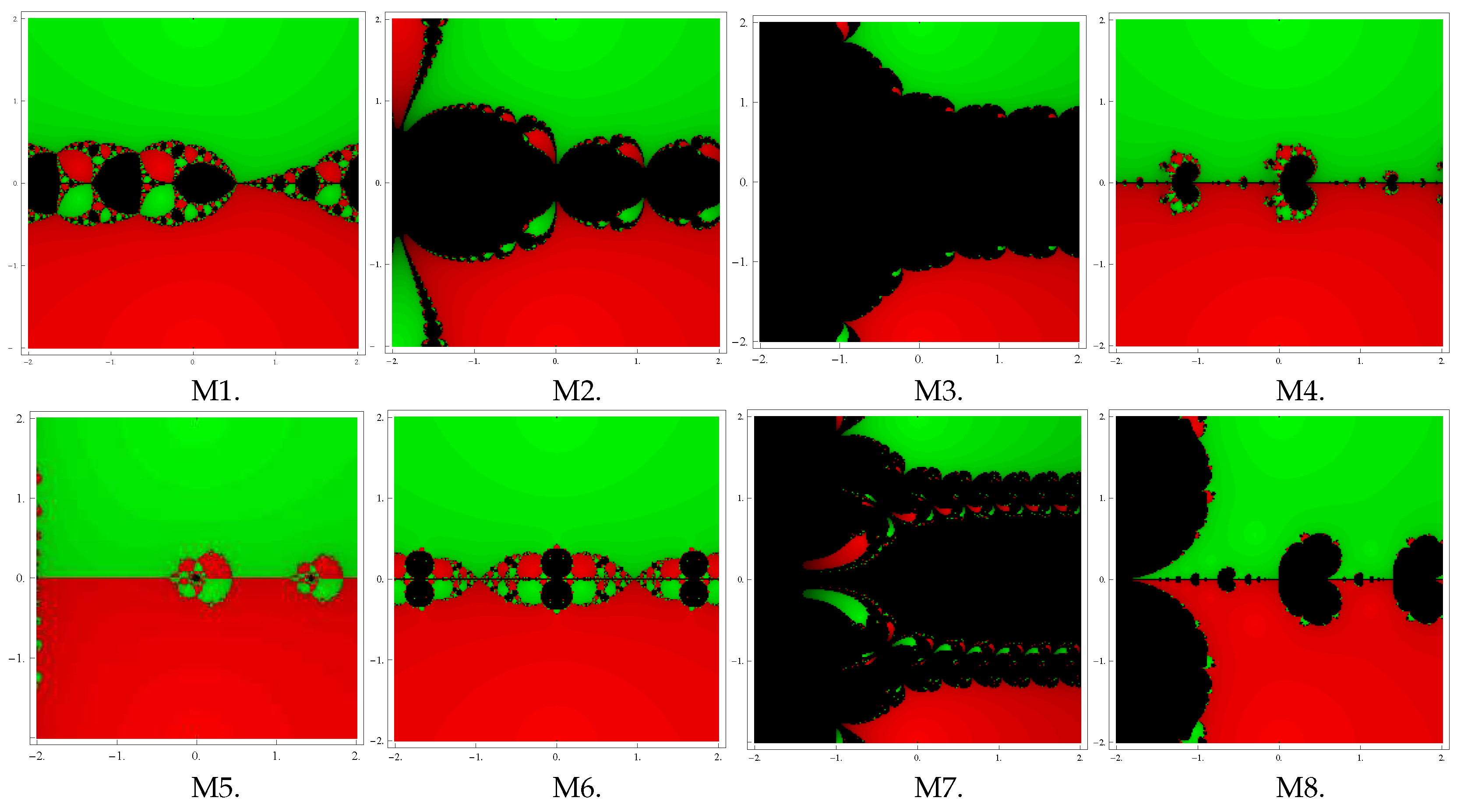
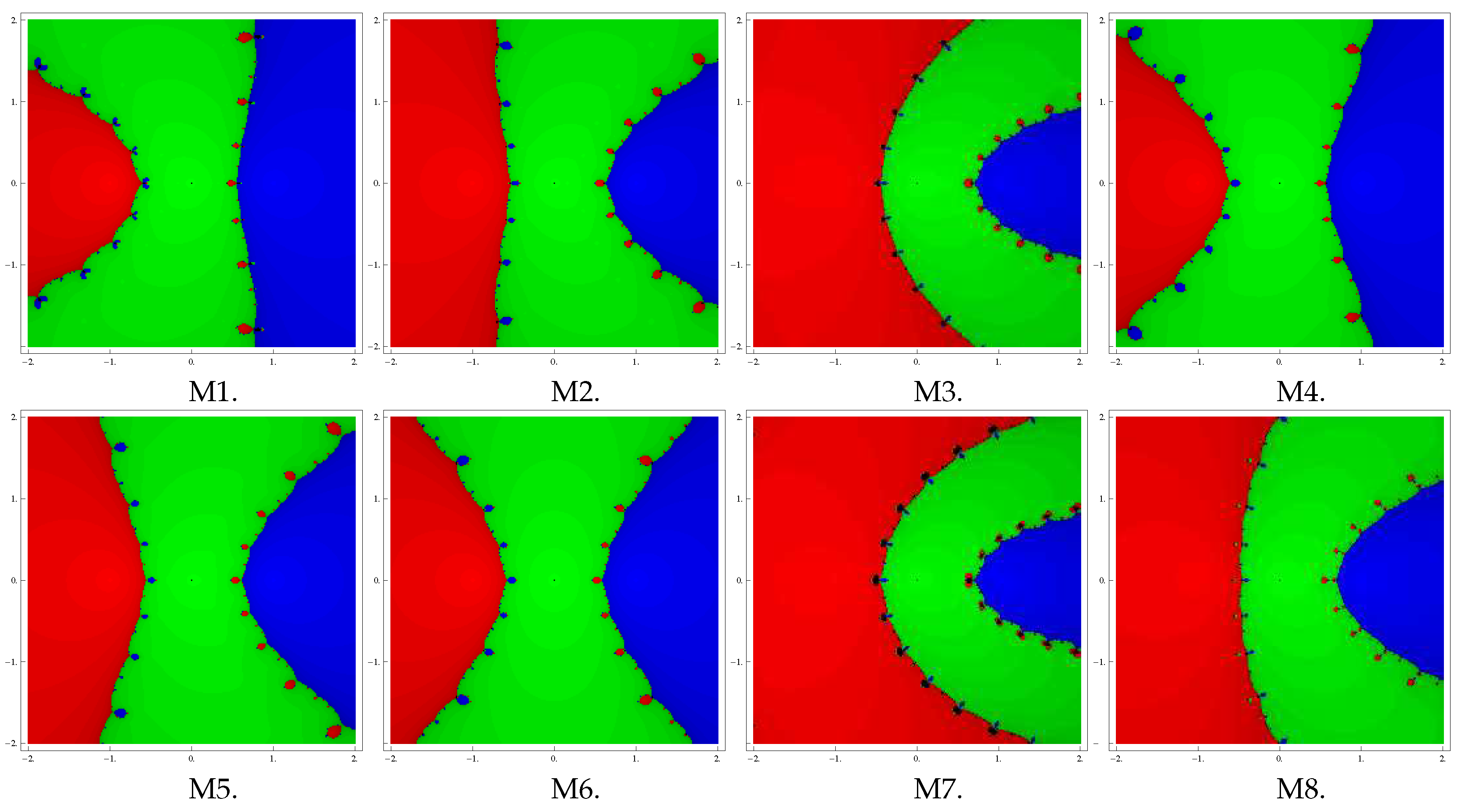
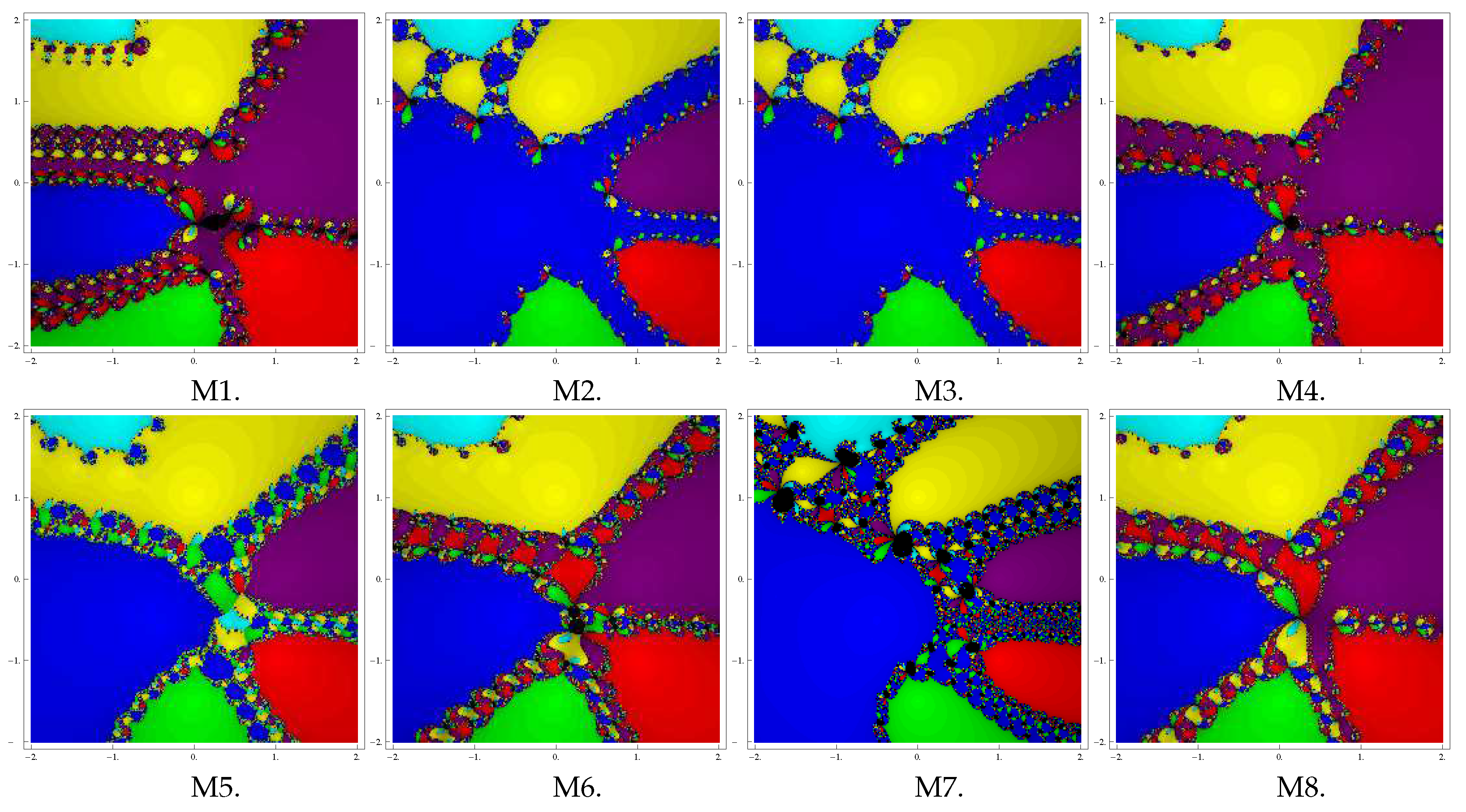
3. Complex Dynamics of Methods

Our goal here is to check the complex dynamics of new methods with the help of a graphical tool, the basins of attraction, of the zeros for a polynomial $P\left(z\right)$ in the Argand plane. The nature of the basins of attraction provides important ideas about the stability and convergence of iterative methods. This idea was initially introduced by Vrscay and Gilbert [29]. In recent times, most researchers have been using this concept in their work—see, for example [30,31]. We consider the special cases corresponding to $G\left(v_n\right)$ of (2) to analyze the basins of attraction.

The starting approximate $z_0$ is taken in a region of rectangular shape $R\in \mathbb{C}$ that contains all the zeros of $P\left(z\right).$ A method, when it starts from point $z_0$ in a rectangle, either converges to zero, $P\left(z\right)$, or eventually diverges. Therefore, the stopping criterion is ${10}^{-3}$ up to a number of 25 iterations.

To show complex geometry, we checked the basins of attraction of the methods M1–M8 on the following four polynomials:

Problem 1.

In this problem, we took the polynomial $P_1\left(z\right)={(z^2+4)}^2$, which has zeros $\{\pm 2i\}$ with a multiplicity of 2. We used a mesh of $400\times 400$ points in a rectangular frame $D\in \mathbb{C}$ of area $[-2,2]\times [-2,2]$, and gave the color green for “$2i$” and red for “$-2i$”. Each initial point from the green region converges towards “$2i$”, and from the red region it converges to “$-2i$”. Basins obtained for the methods M1–M8 are shown in Figure 1. Analyzing the behavior of the methods, we see that the methods M5 and M6 possess lesser numbers of divergent points, followed by M1, M4, M8, and M2. On the contrary, the method M3 has a higher number of divergent points, followed by M7.

Problem 2.

Let us consider the polynomial $P_2\left(z\right)={(z^3-z)}^3$ having zeros $\{0,\pm 1\}$ with a multiplicity of 3. To see the dynamical structure, we considered a rectangular frame $D=[-2,2]\times [-2,2]\in \mathbb{C}$ with $400\times 400$ mesh points, and gave the colors red, green, and blue to each point in the basins of attraction of $-1$, 0, and 1, respectively. Basins obtained for the methods M1–M8 are shown in Figure 2. Analyzing the behavior of the methods, we observe that the methods M5 and M6 have wider convergence regions, followed by M1, M4, M8, M2, M3, and M7.

Problem 3.

Next, consider the polynomial $P_3\left(z\right)={(z^4-6z^2+8)}^2$ that has four zeros $\{\pm 2,\pm 1.414\dots \}$ with a multiplicity of 2. To view attraction basins, we considered a rectangular frame $D=[-2,2]\times [-2,2]\in \mathbb{C}$ with $400\times 400$ mesh points and assigned the colors red, blue, green, and yellow to each point in the basin of $-2$, $-1.414,\dots$, $1.414\dots$, and 2, respectively. Basins obtained for the methods M1–M8 are shown in Figure 3. Observing the behavior of the methods, we see that the methods M5, M8, M2, M3, M4, M1, and M6 possess a lesser number of divergent points, and therefore, they show good convergence. On the contrary, the method M7 has a higher number of divergent points.

Problem 4.

Lastly, we consider the polynomial $P_4\left(z\right)=z^6-\frac{1}{2}{z}^5+\frac{11}{4}(1+i)z^4-\frac{1}{4}(19+3i)z^3+\frac{1}{4}(11+5i)z^2-\frac{1}{4}(11+i)z+\frac{3}{2}-3i$ that has six simple zeros $\{1,-1+2i,-\frac{1}{2}-\frac{i}{2},i,-\frac{3i}{2},1-i\}$. To view the attraction basins, we considered a rectangle $D=[-2,2]\times [-2,2]\in \mathbb{C}$ with $300\times 300$ grid points, and assigned the colors red, green, yellow, blue, cyan, and purple to each point in the basin of 1, $-1+2i$, $-\frac{1}{2}-\frac{1}{2}i$, i, $-\frac{3}{2}i$, and $1-i$, respectively. Basins obtained for the methods M1–M8 are shown in Figure 4. Analyzing the basins of the methods, we observe that the methods M5, M8, M2, M3, M4, and M6 possess a lesser number of divergent points. On the contrary, the methods M1 and M7 have a higher number of divergent points.

From the graphics of the basins, we can give the judgment on the behavior and suitability of any method in the applications. In the event that we pick an initial point $z_0$ in a zone where various basins of attraction contact one another, it is difficult to anticipate which root will be achieved by the iterative technique that begins in $z_0$. Subsequently, the choice of $z_0$ in such a zone is anything but a decent one. Both the dark zones and the zones with various colors are not appropriate for choosing $z_0$ when we need to obtain a specific root. The most appealing pictures showed up when we had extremely intricate borders between basins of attraction. These borders correspond to the cases where the method is more demanding with respect to the initial point.

4. Numerical Results

In this section, we demonstrate the efficiency, effectiveness, and convergence behavior of the family of new methods by applying them to some practical problems. In this view, we take the special cases M1–M8 of the proposed class and choose $(a_1=1/10)$, $(a_2=1/4)$, $(a_3=1/10)$, $(a_4=1/10)$, and $(a_5=1/5)$ in the numerical work.

As we know that the constants $a_1,a_2,a_3,a_4$ and $a_5$ are arbitrary, there is no particular reason for choosing these values for the constants, and we chose the values randomly. The proposed methods are compared with the existing modified Newton Method (1), also known as MNM.

To verify the theoretical results, we calculate the computational order of convergence (COC) by using the formula (see [32])

$$\mathrm{COC}=\frac{log|(x_{n+1}-\alpha )/(x_n-\alpha )|}{log|(x_n-\alpha )/(x_{n-1}-\alpha )|}.$$

The computational work was performed in the programming software, Mathematica, by using multiple-precision arithmetic. Numerical results displayed in

Table 1. Comparison of performance of methods for Example 1.

Methods	n	$|{\mathit{e}}_{\mathit{n}-2}|$	$|{\mathit{e}}_{\mathit{n}-1}|$	$|{\mathit{e}}_{\mathit{n}}|$	$\mathit{f}\left({\mathit{x}}_{\mathit{n}}\right)$	$\mathit{COC}$
MNM	7	$1.70\times {10}^{-21}$	$6.84\times {10}^{-43}$	$1.11\times {10}^{-85}$	$5.90\times {10}^{-681}$	2.000
M1	7	$2.79\times {10}^{-21}$	$1.90\times {10}^{-42}$	$8.77\times {10}^{-85}$	$9.90\times {10}^{-674}$	2.000
M2	7	$2.99\times {10}^{-24}$	$1.56\times {10}^{-48}$	$4.27\times {10}^{-97}$	$8.37\times {10}^{-773}$	2.000
M3	6	$2.17\times {10}^{-13}$	$6.50\times {10}^{-27}$	$5.80\times {10}^{-54}$	$3.68\times {10}^{-428}$	2.000
M4	7	$3.39\times {10}^{-18}$	$4.18\times {10}^{-36}$	$6.32\times {10}^{-72}$	$3.53\times {10}^{-570}$	2.000
M5	6	$5.79\times {10}^{-15}$	$3.77\times {10}^{-30}$	$1.60\times {10}^{-60}$	$5.51\times {10}^{-481}$	2.000
M6	7	$1.93\times {10}^{-21}$	$8.86\times {10}^{-43}$	$1.86\times {10}^{-85}$	$3.69\times {10}^{-679}$	2.000
M7	6	$2.28\times {10}^{-13}$	$7.15\times {10}^{-27}$	$7.03\times {10}^{-54}$	$1.71\times {10}^{-427}$	2.000
M8	7	$6.63\times {10}^{-20}$	$1.26\times {10}^{-39}$	$4.60\times {10}^{-79}$	$1.09\times {10}^{-627}$	2.000

,

Table 2. Comparison of performance of methods for Example 2.

Methods	n	$|{\mathit{e}}_{\mathit{n}-2}|$	$|{\mathit{e}}_{\mathit{n}-1}|$	$|{\mathit{e}}_{\mathit{n}}|$	$\mathit{f}\left({\mathit{x}}_{\mathit{n}}\right)$	$\mathit{COC}$
MNM	7	$1.61\times {10}^{-20}$	$6.50\times {10}^{-41}$	$1.06\times {10}^{-81}$	$1.86\times {10}^{-324}$	2.000
M1	7	$3.37\times {10}^{-21}$	$2.55\times {10}^{-42}$	$1.47\times {10}^{-84}$	$5.64\times {10}^{-336}$	2.000
M2	7	$7.19\times {10}^{-18}$	$1.94\times {10}^{-35}$	$1.41\times {10}^{-70}$	$1.34\times {10}^{-279}$	2.000
M3	7	$2.52\times {10}^{-18}$	$2.22\times {10}^{-36}$	$1.73\times {10}^{-72}$	$2.63\times {10}^{-287}$	2.000
M4	6	$1.85\times {10}^{-22}$	$4.10\times {10}^{-47}$	$2.02\times {10}^{-96}$	$5.76\times {10}^{-388}$	2.000
M5	7	$6.46\times {10}^{-16}$	$2.09\times {10}^{-31}$	$2.17\times {10}^{-62}$	$1.34\times {10}^{-246}$	2.000
M6	7	$1.23\times {10}^{-20}$	$3.75\times {10}^{-41}$	$3.52\times {10}^{-82}$	$2.31\times {10}^{-326}$	2.000
M7	7	$1.35\times {10}^{-17}$	$7.17\times {10}^{-35}$	$2.01\times {10}^{-69}$	$6.02\times {10}^{-275}$	2.000
M8	6	$1.34\times {10}^{-17}$	$9.03\times {10}^{-36}$	$4.08\times {10}^{-72}$	$1.66\times {10}^{-287}$	2.000

,

Table 3. Comparison of performance of methods for Example 3.

Methods	n	$|{\mathit{e}}_{\mathit{n}-2}|$	$|{\mathit{e}}_{\mathit{n}-1}|$	$|{\mathit{e}}_{\mathit{n}}|$	$\mathit{f}\left({\mathit{x}}_{\mathit{n}}\right)$	$\mathit{COC}$
MNM	10	$2.22\times {10}^{-22}$	$8.24\times {10}^{-43}$	$1.13\times {10}^{-83}$	$1.36\times {10}^{-331}$	2.000
M1	10	$1.49\times {10}^{-22}$	$3.70\times {10}^{-43}$	$2.27\times {10}^{-84}$	$2.22\times {10}^{-334}$	2.000
M2	10	$1.52\times {10}^{-21}$	$3.88\times {10}^{-41}$	$2.52\times {10}^{-80}$	$3.43\times {10}^{-318}$	2.000
M3	10	$1.05\times {10}^{-21}$	$1.83\times {10}^{-41}$	$5.64\times {10}^{-81}$	$8.54\times {10}^{-321}$	2.000
M4	10	$3.11\times {10}^{-24}$	$1.59\times {10}^{-46}$	$4.15\times {10}^{-91}$	$2.39\times {10}^{-361}$	2.000
M5	10	$8.82\times {10}^{-21}$	$1.32\times {10}^{-39}$	$2.93\times {10}^{-77}$	$6.32\times {10}^{-306}$	2.000
M6	10	$2.42\times {10}^{-22}$	$9.73\times {10}^{-43}$	$1.58\times {10}^{-83}$	$5.16\times {10}^{-331}$	2.000
M7	10	$1.95\times {10}^{-21}$	$6.42\times {10}^{-41}$	$6.92\times {10}^{-80}$	$1.95\times {10}^{-316}$	2.000
M8	9	$9.79\times {10}^{-17}$	$1.57\times {10}^{-31}$	$4.02\times {10}^{-61}$	$2.10\times {10}^{-241}$	2.000

and

Table 4. Comparison of performance of methods for Example 4.

Methods	n	$|{\mathit{e}}_{\mathit{n}-2}|$	$|{\mathit{e}}_{\mathit{n}-1}|$	$|{\mathit{e}}_{\mathit{n}}|$	$\mathit{f}\left({\mathit{x}}_{\mathit{n}}\right)$	$\mathit{COC}$
MNM	7	$2.87\times {10}^{-15}$	$2.75\times {10}^{-30}$	$2.51\times {10}^{-60}$	$5.82\times {10}^{-478}$	2.000
M1	7	$2.88\times {10}^{-15}$	$2.76\times {10}^{-30}$	$2.53\times {10}^{-60}$	$6.21\times {10}^{-478}$	2.000
M2	7	$3.41\times {10}^{-15}$	$3.95\times {10}^{-30}$	$5.30\times {10}^{-60}$	$2.45\times {10}^{-475}$	2.000
M3	7	$4.43\times {10}^{-15}$	$6.84\times {10}^{-30}$	$1.63\times {10}^{-59}$	$2.14\times {10}^{-471}$	2.000
M4	7	$5.70\times {10}^{-15}$	$1.16\times {10}^{-29}$	$4.75\times {10}^{-59}$	$1.24\times {10}^{-467}$	2.000
M5	7	$5.48\times {10}^{-15}$	$1.07\times {10}^{-29}$	$4.06\times {10}^{-59}$	$3.53\times {10}^{-468}$	2.000
M6	7	$2.99\times {10}^{-15}$	$2.98\times {10}^{-30}$	$2.95\times {10}^{-60}$	$2.10\times {10}^{-477}$	2.000
M7	7	$4.48\times {10}^{-15}$	$6.97\times {10}^{-30}$	$1.69\times {10}^{-59}$	$2.90\times {10}^{-471}$	2.000
M8	7	$3.37\times {10}^{-15}$	$3.82\times {10}^{-30}$	$4.91\times {10}^{-60}$	$1.29\times {10}^{-475}$	2.000

include: (i) the number of approximations $\left(n\right)$ required to converge to the solution such that $|x_{n+1}-x_n|+|f\left(x_n\right)|<{10}^{-100}$, (ii) values of the last three consecutive errors $|e_n|=|x_{n+1}-x_n|$, (iii) residual error $\left|f\right(x_n\left)\right|$, and (iv) computational order of convergence (COC).

For testing, we chose four test problems as follows:

Example 1 (Eigenvalue problem).

Eigen value problem is a difficult problem when characteristic polynomial involves a huge square matrix. Finding the zeros of characteristic equation of a square matrix with order more than 4 can even be a challenging task. So, we think about accompanying 9 × 9 matrix

$$M=\frac{1}{8}\left[\begin{array}{ccccccccc}-12& 0& 0& 19& -19& 76& -19& 18& 437\\ -64& 24& 0& -24& 24& 64& -8& 32& 376\\ -16& 0& 24& 4& -4& 16& -4& 8& 92\\ -40& 0& 0& -10& 50& 40& 2& 20& 242\\ -4& 0& 0& -1& 41& 4& 1& 0& 25\\ -40& 0& 0& 18& -18& 104& -18& 20& 462\\ -84& 0& 0& -29& 29& 84& 21& 42& 501\\ 16& 0& 0& -4& 4& -16& 4& 16& -92\\ 0& 0& 0& 0& 0& 0& 0& 0& 24\end{array}\right].$$

The characteristic polynomial of the matrix $\left(M\right)$ is given as

$$\begin{array}{cc}\hfill h_1\left(x\right)=& x^9-29x^8+349x^7-2261x^6+8455x^5-17663x^4+15927x^3\hfill \\ & +6993x^2-24732x+12960.\hfill \end{array}$$

This function has one multiple zero $\alpha =3$ with a multiplicity of 4. We chose initial approximations $x_0=2.75$ and obtained the numerical results as shown in Table 1.

Example 2 (Beam Designing Model).

Here, we consider a beam situating problem (see [4]) where a beam of length r unit is inclining toward the edge of a cubical box with the length of the sides being 1 unit each, to such an extent that one end of the bar touches the wall and the opposite end touches the floor, as shown in Figure 5.

The problem is: What should be the distance be along the bottom of the beam to the floor from the base of the wall? Suppose y is the distance along the edge of the box to the beam from the floor, and let x be the distance from the bottom of the box and of the beam. Then, for a particular value of r, we have

$$x^4+4x^3-24x^2+16x+16=0.$$

The non-negative solution of the equation is a root $x=2$ with a multiplicity of 2. We consider the initial approximate $x_0=3$ to find the root. Numerical results of various methods are shown in Table 2.

Example 3.

Van der Waals Equation of State, which can be expressed as

$$\left(P+\frac{a_1{n}^2}{V^2}\right)(V-n{a}_2)=nRT,$$

explains the conduct of a real gas by taking in the perfect gas conditions two additional parameters, $a_1$ and $a_2$, explicit for every gas. So as to decide the volume V of the gas as far as the rest of the parameters, we are required to explain the nonlinear condition in V.

$$P{V}^3-(n{a}_{2}P+nRT)V^2+a_1{n}^{2}V-a_1{a}_2{n}^3=0.$$

Given the constants $a_1$ and $a_2$ of a specific gas, one can find values for n, P, and T, with the end goal that this condition has three real roots. By utilizing the specific values, we get the accompanying nonlinear function

$$f1\left(x\right)=x^3-5.22x^2+9.0825x-5.2675,$$

having three real roots. One root among three roots is a multiple zero $\alpha =1.75$ with a multiplicity of order two, and other one being a simple zero $\xi =1.72$. However, our desired zero is $\alpha =1.75$. We considered the initial guess $x_0=1.8$ for this problem. Numerical results of various methods are shown in Table 3.

Example 4.

Lastly, we consider the test function

$$h_4\left(x\right)=\left(x^2+1\right)\left(2x{e}^{x^2+1}+x^3-x\right){cosh}^2\left(\frac{\pi x}{2}\right).$$

The function has a multiple zero $\alpha =i$ of multiplicity 4. We chose the initial approximation $x_0=1.25i$ to obtain the zero of the function.

5. Conclusions

In this paper, we presented a new one-point family of iterative methods with quadratic convergence for computing multiple roots with known multiplicity, based on the weight function technique. Analysis of the convergence showed the second order of convergence under some suppositions regarding the nonlinear function whose zeros are to be obtained. Some efficient and simple cases of the class were presented, and their stability was tested by analyzing complex geometry using a graphical tool—namely, the basin of attraction. The methods were employed to solve some real-world problems, such as the Eigenvalue problem, beam positioning problem, and the Van dar Waal equation of state, and were also compared with existing methods. Numerical comparison of the results revealed that the presented methods had good convergence behavior, similar to the well-known modified Newton’s method.

References

1. Argyros, I.K. Convergence and Applications of Newton-Type Iterations; Springer: New York, NY, USA, 2008. [Google Scholar]
2. Traub, J.F. Iterative Methods for the Solution of Equations; Chelsea Publishing Company: New York, NY, USA, 1982. [Google Scholar]
3. Hoffman, J.D. Numerical Methods for Engineers and Scientists; McGraw-Hill Book Company: New York, NY, USA, 1992. [Google Scholar]
4. Zachary, J.L. Introduction to Scientific Programming: Computational Problem Solving Using Maple and C; Springer: New York, NY, USA, 2012. [Google Scholar]
5. Cesarano, C. Generalized special functions in the description of fractional diffusive equations. Commun. Appl. Ind. Math. 2019, 10, 31–40. [Google Scholar] [CrossRef] [Green Version]
6. Cesarano, C. Multi-dimensional Chebyshev polynomials: A non-conventional approach. Commun. Appl. Ind. Math. 2019, 10, 1–19. [Google Scholar] [CrossRef]
7. Cesarano, C.; Ricci, P.E. Orthogonality Properties of the Pseudo-Chebyshev Functions (Variations on a Chebyshev’s Theme). Mathematics 2019, 7, 180. [Google Scholar] [CrossRef]
8. Schröder, E. Über unendlich viele Algorithmen zur Auflösung der Gleichungen. Math. Ann. 1870, 2, 317–365. [Google Scholar] [CrossRef]
9. Dong, C. A family of multipoint iterative functions for finding multiple roots of equations. Int. J. Comput. Math. 1987, 21, 363–367. [Google Scholar] [CrossRef]
10. Geum, Y.H.; Kim, Y.I.; Neta, B. A class of two-point sixth-order multiple-zero finders of modified double-Newton type and their dynamics. Appl. Math. Comput. 2015, 270, 387–400. [Google Scholar] [CrossRef] [Green Version]
11. Hansen, E.; Patrick, M. A family of root finding methods. Numer. Math. 1977, 27, 257–269. [Google Scholar] [CrossRef]
12. Li, S.; Liao, X.; Cheng, L. A new fourth-order iterative method for finding multiple roots of nonlinear equations. Appl. Math. Comput. 2009, 215, 1288–1292. [Google Scholar]
13. Neta, B. New third order nonlinear solvers for multiple roots. Appl. Math. Comput. 2008, 202, 162–170. [Google Scholar] [CrossRef] [Green Version]
14. Osada, N. An optimal multiple root-finding method of order three. J. Comput. Appl. Math. 1994, 51, 131–133. [Google Scholar] [CrossRef] [Green Version]
15. Sharifi, M.; Babajee, D.K.R.; Soleymani, F. Finding the solution of nonlinear equations by a class of optimal methods. Comput. Math. Appl. 2012, 63, 764–774. [Google Scholar] [CrossRef]
16. Sharma, J.R.; Sharma, R. Modified Jarratt method for computing multiple roots. Appl. Math. Comput. 2010, 217, 878–881. [Google Scholar] [CrossRef]
17. Victory, H.D.; Neta, B. A higher order method for multiple zeros of nonlinear functions. Int. J. Comput. Math. 1983, 12, 329–335. [Google Scholar] [CrossRef]
18. Zhou, X.; Chen, X.; Song, Y. Constructing higher-order methods for obtaining the multiple roots of nonlinear equations. J. Comput. Appl. Math. 2011, 235, 4199–4206. [Google Scholar] [CrossRef] [Green Version]
19. Ostrowski, A.M. Solution of Equations and Systems of Equations; Academic Press: New York, NY, USA, 1966. [Google Scholar]
20. Kung, H.T.; Traub, J.F. Optimal order of one-point and multipoint iteration. J. Assoc. Comput. Mach. 1974, 21, 643–651. [Google Scholar] [CrossRef]
21. Geum, Y.H.; Kim, Y.I.; Neta, B. A sixth–order family of three–point modified Newton–like multiple–root finders and the dynamics behind their extraneous fixed points. Appl. Math. Comput. 2016, 283, 120–140. [Google Scholar] [CrossRef]
22. Behl, R.; Cordero, A.; Motsa, S.S.; Torregrosa, J.R. An eighth-order family of optimal multiple root finders and its dynamics. Numer. Algor. 2018, 77, 1249–1272. [Google Scholar] [CrossRef]
23. Zafar, F.; Cordero, A.; Rana, Q.; Torregrosa, J.R. Optimal iterative methods for finding multiple roots of nonlinear equations using free parameters. J. Math. Chem. 2017. [Google Scholar] [CrossRef]
24. Geum, Y.H.; Kim, Y.I.; Neta, B. Constructing a family of optimal eighth-order modified Newton-type multiple-zero finders along with the dynamics behind their purely imaginary extraneous fixed points. J. Comput. Appl. Math. 2018, 333, 131–156. [Google Scholar] [CrossRef]
25. Behl, R.; Zafar, F.; Alshomrani, A.S.; Junjua, M.; Yasmin, N. An optimal eighth-order scheme for multiple zeros of univariate function. Int. J. Comput. Math. 2019, 16, 1843002. [Google Scholar] [CrossRef]
26. Behl, R.; Alshomrani, A.S.; Motsa, S.S. An optimal scheme for multiple roots of nonlinear equations with eighth-order convergence. J. Math. Chem. 2018. [Google Scholar] [CrossRef]
27. Zafar, F.; Cordero, A.; Torregrosa, J.R. An efficient family of optimal eighth-order multiple root finder. Mathematics 2018, 6, 310. [Google Scholar] [CrossRef]
28. Chicharro, F.I.; Cordero, A.; Garrido, N.; Torregrosa, J.R. Genertaing root-finder iterative methods of second-order: Convergence and stability. Axioms 2019, 8, 55. [Google Scholar] [CrossRef]
29. Vrscay, E.R.; Gilbert, W.J. Extraneous fixed points, basin boundaries and chaotic dynamics for Schröder and König rational iteration functions. Numer. Math. 1988, 52, 1–16. [Google Scholar] [CrossRef]
30. Scott, M.; Neta, B.; Chun, C. Basin attractors for various methods. Appl. Math. Comput. 2011, 218, 2584–2599. [Google Scholar] [CrossRef]
31. Varona, J.L. Graphic and numerical comparison between iterative methods. Math. Intell. 2002, 24, 37–46. [Google Scholar] [CrossRef]
32. Weerakoon, S.; Fernando, T.G.I. A variant of Newton’s method with accelerated third-order convergence. Appl. Math. Lett. 2000, 13, 87–93. [Google Scholar] [CrossRef]
Figure 1. Basins of attraction of M1–M8 for polynomial P 1 ( z ) .
Mathematics 07 00655 g001
Figure 2. Basins of attraction of M1–M8 for polynomial P 2 ( z ) .
Mathematics 07 00655 g002
Figure 3. Basins of attraction of M1–M8 for polynomial P 3 ( z ) .
Mathematics 07 00655 g003
Figure 4. Basins of attraction of M1–M8 for polynomial P 4 ( z ) .
Mathematics 07 00655 g004
Figure 5. Beam situating problem.
Mathematics 07 00655 g005