Bifurcation and Stability Analysis of a System of Fractional-Order Differential Equations for a Plant–Herbivore Model with Allee Effect


1
Department of Mathematics, Kuwait College of Science and Technology, 27235 Kuwait City, Kuwait
2
Mathematics and Science Education Department, Erciyes University, 38039 Kayseri, Turkey
*
Author to whom correspondence should be addressed.
Mathematics 2019, 7(5), 454; https://doi.org/10.3390/math7050454
Submission received: 10 April 2019
/
Revised: 13 May 2019
/
Accepted: 14 May 2019
/
Published: 20 May 2019
(This article belongs to the Special Issue Computational Methods in Applied Analysis and Mathematical Modeling)
Abstract
:This article concerns establishing a system of fractional-order differential equations (FDEs) to model a plant–herbivore interaction. Firstly, we show that the model has non-negative solutions, and then we study the existence and stability analysis of the constructed model. To investigate the case according to a low population density of the plant population, we incorporate the Allee function into the model. Considering the center manifold theorem and bifurcation theory, we show that the model shows flip bifurcation. Finally, the simulation results agree with the theoretical studies.
1. Introduction
Mathematical modeling for various biological problems is considered to be an exciting research area in the discipline of applied mathematics. In the literature, many biological phenomena were modeled and formulated mathematically [1,2,3,4,5,6]. For example, Liu and Xiao established a predator–prey system in discrete time to analyze the local stability and the bifurcation of solutions around the positive equilibrium point [4]. Kangalgil and Kartal analyzed the host–parasite model that led to a system of differential equations of piecewise constant arguments at specific time t, as well as the stability of all obtained equilibrium points; they showed the conditions of flip and Neimark–Sacker bifurcation [6]. Most of these studies are restricted to integer-order differential equations or differential equations with piecewise constant arguments. However, it was seen that many problems in biology, as well as in other fields such as engineering, finance, and economics, could be formulated successfully using fractional-order differential equations [1,5,7,8,9,10,11,12,13].
The nonlocal property of fractional-order models not only depends on the current state but also depends on its prior historical states [14]. The transformation of an integer-order model into a fractional-order model needs to be precise with respect to the order of differentiation . However, a small change in may cause a big change in the behavior of the solutions [15].
Fractional-order differential equations can model complex biological phenomena with non-linear behavior and long-term memory, which cannot be represented mathematically by integer-order differential equations (IDEs) [16,17]. For example, Bozkurt established the glioblastoma multiforme (GBM)–immune system (IS) interaction using a fractional-order differential equation system to include the delay time (memory effect) [5].
In general, the origin of plant–herbivore interactions is derived from predator–prey systems [18,19], which is described in many studies using discrete and continuous time [6,20,21,22,23]. The usual discrete host–parasite models have the form
where and are the densities of the host (a plant) and the parasite (a herbivore), is the host’s inherent rate of increase where is the intrinsic rate of increase) in the absence of the parasites, is the biomass conversion constant, and is the function defining the fractional survival of hosts from parasitism [21].
In Reference [23], the authors considered a system of differential equations of plant–herbivore interactions as follows:
Kartal in Reference [20] generalized the system in Equation (2) by combining discrete and continuous time as follows:
where and denote the populations of the plant and herbivore, respectively, is the integer part of and the parameters belonging to , is the growth rate, is the carrying capacity, and is the predation rate of the plant species, while and represent the death rate and conversion factor of the herbivores, respectively.
In our study, we consider a model as a system of FDEs as follows:
where represents the Holling type II function given by
In Equation (4), is the growth rate of the plant population, denotes the carrying capacity, denotes the predation rate of the plant species, is the conversion of consumed plant biomass into new herbivore biomass, and is the per capita rate of death. In Equation (5), is the encounter rate, which depends on the movement velocity of the herbivore species. The parameter is the fraction of food items encountered that the herbivore ingests, while is the handling time for each prey item, which incorporates the time required for the digestive tract to handle the item.
Definition 1.
[24] Let be a function, where the fractional integral of orderis given by
provided the right side is pointwise defined on
Definition 2.
[24] Let be a continuous function. The Caputo fractional derivative of order is given by
2. Stability Analysis
2.1. Equilibrium Points
Let us consider the system
We want to discuss the stability of the system in Equation (8). Let us perturb the equilibrium point by adding and , that is
Thus, we have
and
Using the fact we obtain a linearized system about such as
where , and J is the Jacobian matrix evaluated at the point ,
We have , where C is a diagonal matrix of J given by
where and are the eigenvalues and B represents the eigenvectors of J. Therefore, we get
whose solutions are given by the following Mittag–Leffler functions:
and
Using the result of Reference [25], if and then and are decreasing; consequently, and are decreasing. Let the solution of Equation (12) exist. If the solution of Equation (12) is increasing, then is unstable; otherwise, if is decreasing, then is locally asymptotically stable. The equilibrium points of the system in Equation (8) are
where and .
2.2. Local Stability
The Jacobian matrix for the system in Equation (8) is given as
For we have the characteristic equation
Theorem 1.
Let be the extinction point of the system in Equation (8). Then, the equilibrium point of the system in Equation (8) is a saddle point.
For the case where only the plant population exists, we consider the equilibrium point The characteristic equation around is as follows:
Theorem 2.
Assume that is the equilibrium point of the system in Equation (8). Then, the following statements are true:
- (i)
- For , if , then is locally asymptotically stable;
- (ii)
- For , if then is an unstable saddle point.
To discuss the local stability of which means a plant–herbivore interaction exists, we consider the linearized system of the system in Equation (8) at From the Jacobian matrix of Equation (8),
we obtain the characteristic equation
where
By considering Equation (21), we obtain the theorem below.
Theorem 3.
Let the system in Equation (8) have a positive equilibrium point Then, the following statements are true:
- (i)
- Assume that and , where . Ifthen we either attain real or complex conjugates roots with negative real parts, where > is equivalent to the Routh–Hurwitz case. Thus, is locally asymptotically stable;
- (ii)
- Assume that and , where . Ifthen we attain complex conjugates with positive real parts andwhich implies that is locally asymptotically stable.
Proof.
- (i)
- Let us consider the case where . Fromwe havewhere Furthermore, computations show that, forwe obtain , where . In this case, we have .
Since , it is obvious that . This completes the proof of (i).
- (ii)
- Let us consider the case, where . In this case, we havewhere
Furthermore, if
then and , which implies that .
This completes the proof of the theorem. □
Example 1.
In this section, we analyze the stability conditions for the system in Equation (8) that shows a plant–herbivore model with fractional-order differential equations. The values of the parameters are and , where the order of the system is . In Figure 1, we obtain the bifurcation structure of the system in Equation (8) for the initial values , where the blue graph represents the plant population, and the red graph denotes the herbivore population. Obviously, an increase in the plant population allows the herbivore population to increase. After that, an interaction between both populations occurs. Figure 2 is the per capita for each population, which shows that, after a specific capacity of the habitat, the herbivore population will not be able to find enough food, and this may lead to death or migration.
3. Existence and Uniqueness
Considering the system in Equation (8) with initial conditions and , the initial value problem can be written in the form
where and . Let us assume and when . In this case, the initial value problem can be written as
Definition 3.
Assume that is the class of continuous column vector whose components are the class of continuous functions on The norm of is given by When we write and .
Definition 4.
is a solution of the initial value problem in Equation (27) if (i) and (ii) hold.
- (i)
- , where
- (ii)
- satisfies Equation (27).
If Definition 4 holds, we obtain the theorem below.
Theorem 4.
Let be a solution of the initial value problem given in Equation (27). Then, is a unique solution for Equation (27).
Proof.
Let us write
Operating with , we obtain
Now, let be defined by
Then,
This implies that If we choose such that then we obtain , and the operator given by Equation (31) has a unique fixed point.
Consequently, Equation (30) has a unique solution From (30), we have
and
from which we can deduce that Thus, we have
and .
Therefore, this initial value problem is equivalent to the initial value problem in Equation (27). □
4. Analyzing the Plant–Herbivore Population at Low Density
Allee in 1931 established an important role in the dynamical behavior of populations. He showed that population dynamics with logistic equations in a low population size should be modified with the Allee function in order to represent a realistic phenomenon [26].
By considering the logistic equation, the density increases when the per capita growth rate decreases monotonically; however, it is shown that, in logistic population models with the Allee effect, the per capita growth rate increases to a maximum point at low population density and decreases when the density of the population increases [26]. Many theoretical and laboratory studies showed the essential need of the Allee effect in small populations. Based on the biological studies, the following assumptions are necessary for defining the Allee function:
Considering the conditions above, we apply an Allee function at time to the system in Equation (8) as follows:
where and Moreover, we define as the Allee coefficient of the plant population, and is the Allee function. The herbivore population is dependent on the plant population. Thus, if
then the plant population is not sufficient for the herbivore to exist.
For a low population size of the plant population, let us consider the stability conditions around . The Jacobian matrix at is given by
Thus, we obtain the characteristic equation
where and
Theorem 5.
Let the system in Equation (32) have a positive equilibrium point Then, the following statements are true:
- (i)
- Assume that and , where . Ifthen we either attain real roots or complex conjugates with negative real parts, where > is equivalent to the Routh–Hurwitz case, which means that is locally asymptotically stable;
- (ii)
- Assume that and , where . Ifthen both roots are complex conjugates with positive real parts andwhich implies that is locally asymptotically stable.
Proof.
- (i)
- Let us consider the case where . Sincewe havewhere Furthermore, fromwe have , where . Thus, . Additionally, it is obvious that . This completes the proof of (i).
- (ii)
- Let us consider the case where . In this case, we havewhere Ifthen and , which implies that . This completes the proof of the theorem. □
Theorem 6.
The system in Equation (32) has a unique solution in if
and
Proof.
Let be a solution of the initial values problem in Equation (32), which holds where and The Equation (32) can be written as
By operating both sides with , we get
Let us define the operator by
From Equation (47), we can write
Therefore, we have
which gives
Thus, if we choose such that we obtain
Moreover, we can obtain
If we choose such that then
Similarly, one can show that Equation (46) is equivalent to the initial value problem in Equation (32). This completes the proof. □
Example 2.
The values of the chosen parameters are similar to those in Example 1. The blue graph represents the plant population, while the red graph denotes the herbivore population. The Allee coefficient is given by . Figure 3 shows the bifurcation structure of the system in Equation (32) under the initial values . Figure 4 shows the per capita for the plant–herbivore population. We realized that, for a low density of the plant population, the dearth or migration of the herbivore population will occur earlier than expected. The plant population can recover after the herbivore population disappears from that habitat.
5. Flip Bifurcation with Discretization Process
In this section, we consider at first the discretization process and the analysis of flip bifurcation. This discretization is an approximation for the right-hand side of the fractional differential equation where . We modify our system in Equation (8) in considering the discrete time effect on the model.
The discretization of Equation (8) is as follows:
For , we have
The solution of Equation (49) reduces to
Let , where we obtain
In repeating the discretization process n times, we get
For , while and , we have
The Jacobian matrix of Equation (53) at the equilibrium points is
where is the positive equilibrium point of Equation (53).
Theorem 7.
Let be the equilibrium point of the system in Equation (53) and assume that i.e.,
If
where and then is local asymptotically stable.
Proof.
The characteristic equation of is of the form
where
and
From Equations (58) and (59), we have
Thus, the characteristic equation of has two eigenvalues, which are
If both and , then the equilibrium point is locally asymptotically stable. From
we obtain
where and . For , Equation (61) can be rewritten as follows:
where we obtain
From
we have
Considering Equations (63) and (65) together, we obtain
This completes the proof. □
Consider , where
The theorem below shows flip bifurcation of the equilibrium point when the parameters vary in the small neighborhood of .
Theorem 8.
Let be the equilibrium point of the system in Equation (53). If the Equation (53) undergoes flip bifurcation. Furthermore, if then the bifurcation of the second period points is stable, while, for , it shows an unstable behaviour.
Proof.
In Theorem 7, we consider the analysis in a neighborhood given as . Let and be a perturbation of the parameter. The perturbed form of Equation (53) is as follows:
For and , the system in Equation (67) can be formulated as
where
For , the eigenvectors of that correspond to the eigenvalues and are
where and .
Here, we choose and . Then, we have an invertible matrix
Let us consider the following transformation:
Taking on both sides of Equation (68), we have
where
and
Let us formulate the center manifold at the point in a neighbourhood of . Let us have a center manifold such as , where
and
which satisfy
Thus, we have
where
and
Example 3.
By considering the same parameter values given in the previous examples, and according to the conditions of Theorem 8, we illustrate Example 3 by changing the carrying capacity of the plant population. Figure 5 and Figure 6 demonstrate the phase plane portraits of the system in Equation (8) for the carrying capacity values.
6. Conclusions
In this paper, the biological dynamics of fractional-order differential equations in a plant–herbivore model was discussed and analyzed. The local stability of the obtained equilibrium points and the existence and uniqueness of the solution in the system in Equation (27) were analyzed (see Example 1). An impressive result was considered in Section 4 where we found that, for a low size of the plant population, the herbivore population disappears. We noticed that the plant–herbivore model is mainly dependent on the plant population size and carrying capacity (see Example 2). On the other hand, we investigate possible bifurcation types, where we saw that the system exhibits a flip bifurcation structure (Section 5). Similar bifurcation studies were observed in many plant–herbivore models such as in References [4,17], where they obtained periodic or quasi-periodic solutions. Finally, we conclude that the environmental carrying capacity of the plant population has a strong effect on the system in Equation (27), while the density of the plant species shows an essential effect for the system in Equation (32). The numerical simulations were carried out using Matlab 2018.
Author Contributions
F.B.Y. conceived the study and was in charge of overall direction and planning. F.B.Y. and A.Y. designed the model and set up the main parts of the study. F.B.Y. and A.Y. set up the theorems and proved them together. They collected and analyzed the data. Both authors interpreted the data and carried out this implementation. A.Y. carried the simulations using Matlab 2018. F.B.Y. and A.Y. wrote the manuscript and revised it to the submitted form. There was no ghost-writing.
Funding
This research received no external funding.
Conflicts of Interest
There are no political, personal, religious, ideological, academic, or intellectual competing interests. The authors declare no competing interests.
References
- Abdelaziz, M.A.; Ismail, A.I.; Abdullah, F.A.; Mohd, M.H. Bifurcation and chaos in a discrete SI epidemic model with fractional order. Adv. Differ. Equ. 2018, 44, 1–19. [Google Scholar] [CrossRef]
- Mena-Lorca, J.; Hethcote, H.W. Dynamic models of infectious diseases regulators of population sizes. J. Math. Biol. 1992, 30, 693–716. [Google Scholar] [PubMed]
- Fend, Z.; Thieme, H.R. Recurrent outbreaks of childhood diseases revised: The impact of isolation. Math. Biosci. 1995, 32, 3–130. [Google Scholar]
- Liu, X.; Xiao, D. Complex dynamic behaviors of a discrete-time predator-prey system. Chaossolutions Fractals 2007, 32, 80–94. [Google Scholar] [CrossRef]
- Bozkurt, F. Stability analysis of a fractional order differential equation system of a GBM-IS interaction depending on the density. Appl. Math. Inf. Sci. 2014, 8, 1–8. [Google Scholar] [CrossRef]
- Kangalgil, F.; Kartal, S. Stability and bifurcation analysis in a host-parasitoid model with Hassell growth function. Adv. Differ. Equ. 2018, 240, 1–15. [Google Scholar] [CrossRef]
- Magin, R.; Ortigueira, M.D.; Podlubny, I.; Trujillo, J. On the fractional signal systems. Signal Process 2011, 91, 350–371. [Google Scholar] [CrossRef]
- Huang, C.; Cao, J.; Xiao, M.; Alsaedi, A.; Hayat, T. Bifurcations in a delayed fractional complex-valued neural network. Appl. Math. Comput. 2017, 292, 210–227. [Google Scholar] [CrossRef]
- Huang, C.; Cao, J.; Xiao, M.; Alsaedi, A.; Alsaadi, F.E. Controlling bifurcation in a delayed fractional predator-prey system with incommensurate orders. Appl. Math. Comput. 2017, 293, 293–310. [Google Scholar] [CrossRef]
- Huang, C.; Cao, J.; Xiao, M.; Alsaedi, A.; Hayat, T. Effects of time delays on stability and Hopf bifurcation in a fractional order ring-structured network with arbitrary neurons. Commun. Nonlinear Sci. Numer. Simul. 2018, 57, 1–13. [Google Scholar] [CrossRef]
- Youssef, I.K.; El Dewaik, M.H. Solving Poisson’s Equations with Fractional Order Using Haaravelet. Appl. Math. Nonlinear Sci. 2017, 2, 271–284. [Google Scholar] [CrossRef]
- Brzezinski, D.W. Comparison of fractional order derivatives computational accuracy-right hand vs left hand definition. Appl. Math. Nonlinear Sci. 2017, 2, 237–248. [Google Scholar] [CrossRef]
- Brzezinski, D.W. Review of numerical methods for NumILPT with computational accuracy assessment for fracional calculus. Appl. Math. Nonlinear Sci. 2018, 3, 487–502. [Google Scholar] [CrossRef]
- Al-Khaled, K.; Alquran, M. An approximate solution for a fractional order model of generalized Harry Dym equation. Math. Sci. 2014, 8, 125–130. [Google Scholar] [CrossRef]
- Bagley, R.L.; Calico, R.A. Fractional order state equations for the control of viscoelastically damped structures. J. Guid. Control Dyn. 1991, 14, 304–311. [Google Scholar] [CrossRef]
- Ichise, M.; Nagayanagi, Y.; Kojima, T. An analog simulation of non-integer order transfer functions for analysis of electrode process. J. Electroanal. Chem. Interfaction Electrochem. 1971, 33, 253–265. [Google Scholar] [CrossRef]
- Ahmad, W.M.; Sprott, J.C. Chaos in fractional order autonomous nonlinear systems. Chaos Solutions Fractals 2003, 16, 339–351. [Google Scholar] [CrossRef]
- Caughley, G.; Lawton, J.H. Plant-herbivore systems. In Theoretical Ecology; Principles and Applications; May, R.M., Ed.; Blackwell Scientific Publications: Blackwell, Oxford, UK, 1981; pp. 132–166. [Google Scholar]
- May, R.M. Stability and Complexity in Model Ecosystems; Princeton University Press: Princeton, NJ, USA, 2011. [Google Scholar]
- Kartal, S. Dynamics of a plant-herbivore model with differential-difference equations. Cogent Math. 2016, 3, 1–9. [Google Scholar] [CrossRef]
- Kang, Y.; Armbruster, D.; Kuang, Y. Dynamics of plant-herbivore model. J. Biol. Dyn. 2008, 2, 89–101. [Google Scholar] [CrossRef]
- Agiza, H.N.; Elabbasy, E.M.; El-Metwally, H.; Elsadany, A.A. Chaotic dynamics of a discrete prey-predator model with Hollingen type II. Nonlinear Anal. Real World Appl. 2009, 10, 116–129. [Google Scholar] [CrossRef]
- Chattopadhayay, J.; Sarkar, R.; Fritzsche-Hoballah, M.E.; Turlings, T.C.; Bersier, L.F. Parasitoids may determine plant fitness-A mathematical model based on experimental data. J. Theor. Biol. 2001, 212, 295–302. [Google Scholar] [CrossRef] [PubMed]
- Podlubny, I. Fractional Differential Equations; Academic Press: New York, NY, USA, 1999. [Google Scholar]
- Matignon, D. Stability results for fractional differential equations with applications to control processing. Proceeding of IMACS-IEE/SMC Conference on Computational Engineering in Systems Applications, Lille, Frace, 9–12 July 1996; 2, pp. 963–968. [Google Scholar]
- Allee, W.C. Animal Aggregations: A Study in General Sociology; University of Chicago Press: Chicago, IL, USA, 1931. [Google Scholar]
- Wang, G.; Liang, X.G.; Wang, F.Z. The competitive dynamics of populations subject to an Allee Effect. Ecol. Model. 1999, 124, 183–192. [Google Scholar] [CrossRef]
- Lande, R. Extinction threshold in demographic models of territorial. Am. Nat. 1987, 130, 624–635. [Google Scholar] [CrossRef]
- Dennis, B. Allee Effect: Population growth, critical density, and change of extinction. Nat. Resour. Model 1989, 3, 481–538. [Google Scholar] [CrossRef]
- Asmussen, M.A. Density-dependent selection II. The Allee Effect. Am. Naturalist 1979, 14, 796–809. [Google Scholar] [CrossRef]
- Bozkurt, F.; Abdeljawad, T.; Hajji, M.A. Stability analysis of a fractional order differential equation model of a brain tumor growth depending on the density. Appl. Comput. Math. 2015, 14, 1–13. [Google Scholar]
- Yuang, L.G.; Yang, Q.G. Bifurcation, invariant curve and hybrid control in a discrete-time predator-prey system. Appl. Math. Model. 2015, 39, 2345–2362. [Google Scholar] [CrossRef]
Figure 1.
Plant–herbivore bifurcation diagram.
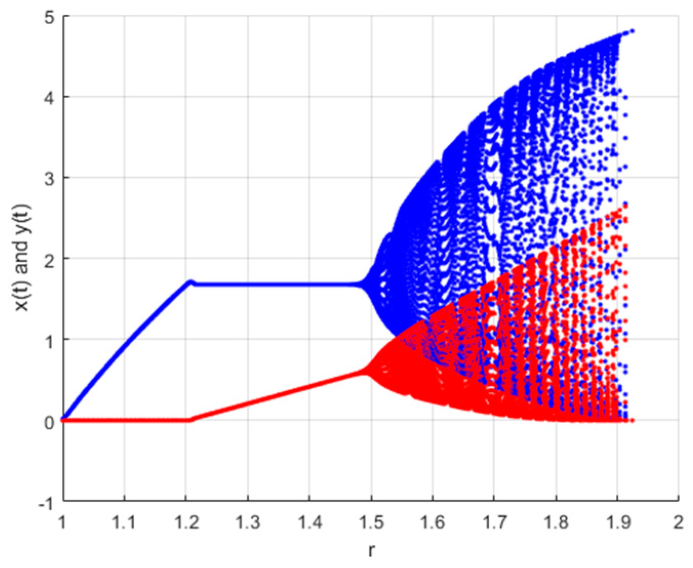
Figure 2.
Per capita of plant–herbivore population.

Figure 3.
Plant–herbivore bifurcation diagram.

Figure 4.
Per capita of plant–herbivore population.
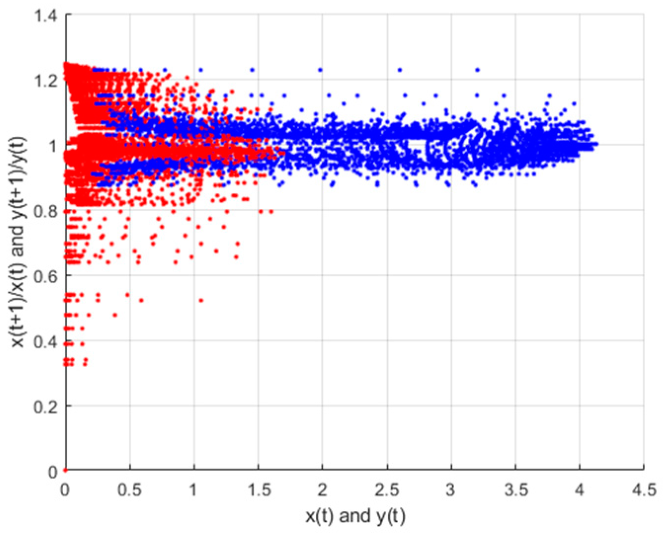
Figure 5.
Phase plane for .
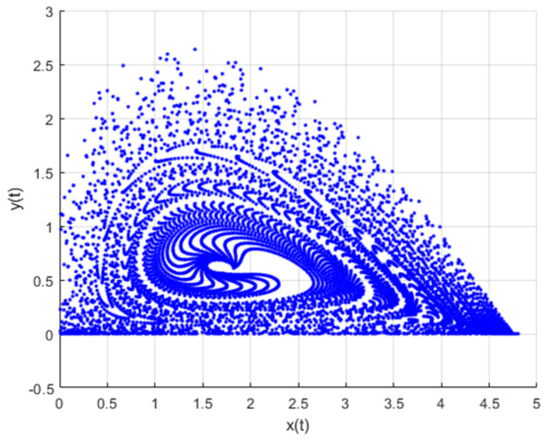
Figure 6.
Phase plane for .

© 2019 by the authors. Licensee MDPI, Basel, Switzerland. This article is an open access article distributed under the terms and conditions of the Creative Commons Attribution (CC BY) license (http://creativecommons.org/licenses/by/4.0/).
Share and Cite
MDPI and ACS Style
Yousef, A.; Yousef, F.B. Bifurcation and Stability Analysis of a System of Fractional-Order Differential Equations for a Plant–Herbivore Model with Allee Effect. Mathematics 2019, 7, 454. https://doi.org/10.3390/math7050454
AMA Style
Yousef A, Yousef FB. Bifurcation and Stability Analysis of a System of Fractional-Order Differential Equations for a Plant–Herbivore Model with Allee Effect. Mathematics. 2019; 7(5):454. https://doi.org/10.3390/math7050454
Chicago/Turabian StyleYousef, Ali, and Fatma Bozkurt Yousef. 2019. "Bifurcation and Stability Analysis of a System of Fractional-Order Differential Equations for a Plant–Herbivore Model with Allee Effect" Mathematics 7, no. 5: 454. https://doi.org/10.3390/math7050454
Note that from the first issue of 2016, this journal uses article numbers instead of page numbers. See further details here.