Article

A Multiscale RBF Collocation Method for the Numerical Solution of Partial Differential Equations

1
School of Mathematical Sciences, Fudan University, Shanghai 200433, China
2
school of Mathematics and Statistics, Ningxia University, Yinchuan 750021, China
*
Author to whom correspondence should be addressed.
Mathematics 2019, 7(10), 964; https://doi.org/10.3390/math7100964
Submission received: 10 September 2019 / Revised: 7 October 2019 / Accepted: 10 October 2019 / Published: 13 October 2019
(This article belongs to the Section Mathematics and Computer Science)

Abstract

:
In this paper, we derive and discuss the hierarchical radial basis functions method for the approximation to Sobolev functions and the collocation to well-posed linear partial differential equations. Similar to multilevel splitting of finite element spaces, the hierarchical radial basis functions are constructed by employing successive refinement scattered data sets and scaled compactly supported radial basis functions with varying support radii. Compared with the compactly supported radial basis functions approximation and stationary multilevel approximation, the new method can not only solve the present problem on a single level with higher accuracy and lower computational cost, but also produce a highly sparse discrete algebraic system. These observations are obtained by taking the direct approach of numerical experimentation.
MSC:
Primary 65J10; 65N15; 65N35; 65N55

1. Introduction

In this paper, we introduce the hierarchical radial basis functions method for the approximation to Sobolev functions and the collocation to well-posed linear partial differential equations. Hierarchical basis may be a common concept in finite element books, which is formed by decomposing finite element spaces (see an earlier paper by Yserentant, in 1986 [1]). Hierarchical radial basis functions network is a concept in neural networks, which is an approximating neural model and is a self-organizing (by growing) multiscale version of a radial basis function network. In this paper, hierarchical radial basis functions (H-RBFs) refer to some basis functions that are constructed by employing hierarchical data structure and scaled compactly supported radial basis functions. Below, we can explain why hierarchical radial basis functions are necessary.
As the first kernel-based collocation method was introduced by Kansa [2], radial basis functions have been successfully applied to solving various partial differential equations numerically. However, unfortunately, we are obtaining highly accurate solutions from severely ill-conditioned linear systems and high computational cost when using radial basis functions collocation methods. This is a well-known uncertainty or trade-off principle [3]. To overcome this problem, different strategies have been suggested, see a summary of existing methods in the recent monograph [4]. There are about three kinds of popular methods to deal with this problem.
The first method is finding optimal shape parameter ε (which is related to the scattered centers distribution, and usually is inversely proportional to mesh norm). We have become accustomed to scaling one of radial functions through multiplying the independent variable · by a shape parameter ε in the practical approximation. Obviously, a smaller value of ε causes the function to become flatter, whereas increasing ε leads to a more peaked radial function, and therefore localizes its influence. The choice of ε has a profound influence on both the approximation accuracy and numerical stability of the solution to interpolation problem. The general observation was that a large ε leads to a very well-conditioned linear system but also a poor approximation rate, whereas a smaller ε yields excellent approximation at the price of a badly conditioned system. A number of strategies for choosing a “good” value of ε have been suggested, such as the power function as indicator, the Cross Validation algorithm and the Contour–Padé algorithm. Some discussion of the existing parametrization schemes is provided in books [4,5]. Madych [6] indicated that the interpolation error goes to zero as ε 0 , this does not seem to be true in practice. Beyond that, there is no case known where the error and the sensitivity are both reasonably small.
The second method is the utilization of compactly supported radial basis functions (CSRBFs). Since 1995, a series of compactly supported radial basis functions have emerged gradually, such as Wendland’s function [7], Wu’s function [8], Buhmann’s function [9], and others [5]. The compact support automatically ensures the strict positive definiteness of CSRBFs. However, an additional trade-off principle remains, now depending on the choice of the support size. Specifically, a small support leads to a well-conditioned system but also poor approximation accuracy, whereas a larger support yields excellent accuracy at the price of ill-conditioned system.
The third method is stationary multilevel interpolation. With a stationary multiscale algorithm [10], the condition number of the discrete matrix can be relatively small, and computation can be performed in O ( N ) operations. In this method, the present problem (interpolation or numerical PDEs) is solved first on the coarsest level by one of the compactly supported radial basis functions with a larger support (usually scaling the size of the support with the fill distance). Then, the residual can be formed, and then computed on the next finer level by the same compactly supported radial basis function but with a smaller support. This process can be repeated and be stopped on the finest level. The final approximation is the sum of all of interpolants. For interpolation problems, the linear convergence order has been proved in Sobelev spaces on the sphere in [11], and on bounded domains in [12]. Applications of this algorithm in solving PDEs on spheres are proposed in [13], on bounded domains were proposed in [14,15,16]. However, a series of global interpolation or approximation problems must be solved on different levels, although two kinds of local algorithms have been derived in [17,18] recently.
This paper considers solving the present problem on a single level. At the current scattered data set the trial function is represented as linear combination of hierarchical radial basis functions. The approximation method can produce a sparse discrete algebraic system, because hierarchical radial basis functions are derived from CSRBFs with different support radii. Compared with compactly supported radial basis functions approximation [7,8] and stationary multilevel approximation [11,12,13,14,15,16,17,18], the new method can solve the present problem on a single level with higher accuracy and lower computational cost. The effectiveness of H-RBFs collocation method will be conformed by several numerical observations.

2. H-RBFs Trial Spaces

In this section, we build H-RBFs trial spaces and assemble the discrete spaces with appropriate norms. In particular, we will prove two norm equivalence theorems and describe a function spaces commuting diagram. To avoid writing constants repeatedly, we shall use notations ≲ and ≅. Short notation x y means x C 1 y , and x y means C 1 x y C 2 x , and C 1 and C 2 are positive constants.

2.1. H-RBFs Trial Spaces

Let X = { x 1 , , x N } be a finite point set in Ω R d . We define a commonly used trial discretization parameter:
h X , Ω : = sup x Ω min x j X x x j 2 ,
which can be regarded as the radius of the largest empty ball that can be placed among the data sites x j . To build H-RBFs trial spaces, we need the nested point sets
X 1 X 2 X j
which have trial discretization parameters h j = h X j , Ω . Let X j * be newly added point set in X j , then we have X 1 = X 1 * and X j = X j 1 X j * for j = 2 , .
Given a kind of the compactly supported radial functions Φ : R d R , we can rescale it (by a scaling parameter ε j > 0 , and in the translation-invariant kernel-based case) as
Φ j ( · , y ) = ε j d Φ ( ε j ( · y ) ) , y X j * .
To make the support radii of Φ j become smaller and smaller with the addition of new points, we select
ε j = b 1 h j , with   a   given   constant 0 < b 1 .
Let V j = V j 1 W j , with V 1 = W 1 and W j = span { Φ j ( · , y ) : y X j * } for j = 1 , . Then we can build the H-RBFs trial spaces of the form
V j = span { Φ 1 ( x , x 1 1 ) , , Φ 1 ( x , x 1 M 1 ) , , Φ j ( x , x j 1 ) , , Φ j ( x , x j M j ) } ,
which differs from the RBFs approximation spaces
U j = span { Φ ( x , x 1 1 ) , , Φ ( x , x 1 M 1 ) , , Φ ( x , x j 1 ) , , Φ ( x , x j M j ) } .
Here, we have written X k * = { x k 1 , , x k M k } for k = 1 , 2 , , j .

2.2. Norms of the Discrete Spaces V j

The following is a relation between several function spaces.
W m , 2 ( Ω ) ( 3 ) When Φ ^ decays only algebraically with m > d 2 N Φ ( Ω ) ( 2 ) When Φ is strictly positive definite H Φ ( Ω ) ( 1 ) When point evaluation functionals are continuous H ( Ω )
Adding a restrictive condition (1), the Hilbert space H ( Ω ) becomes the reproducing kernel Hilbert space H Φ ( Ω ) with reproducing Φ : Ω × Ω R . N Φ ( Ω ) is a reproducing kernel Hilbert space with a strictly positive definite kernel Φ . N Φ ( Ω ) is the native space of Φ , which contains all functions of the form g = j = 1 N c j Φ ( · , x j ) provided x j Ω , with
g N Φ ( Ω ) 2 = j = 1 N k = 1 N c j c k Φ ( x j , x k ) .
When Ω = R d , we get a characterization of N Φ ( R d ) in terms of the Fourier transforms
g N Φ ( R d ) 2 = R d | g ^ ( ω ) | 2 Φ ^ ( ω ) d ω , g L 2 ( R d ) .
Here
Φ ^ ( ω ) = ( 2 π ) d 2 R d Φ ( x ) e i x T ω d x .
In fact, there exist such radial functions whose Fourier transforms decay only algebraically, satisfying
Φ ^ ( ω ) 1 + ω 2 2 τ , ω R d .
Then, scaled radial functions Φ j ( x ) = ε j d Φ ( ε j x ) have Fourier transforms satisfying
Φ j ^ ( ω ) 1 + 1 ε j 2 ω 2 2 τ , ω R d .
To clarify the relation between Sobolev spaces and native spaces, we cite the following extension operator theorems.
Theorem 1.
(Sobolev extension operator, see Section 5.17 in [19].)
Suppose Ω R d is open and has a Lipschitz boundary. Let τ 0 . Then. for all g H τ ( Ω ) , there exists a linear operator, E : H τ ( Ω ) H τ ( R d ) , such that
(1) E g | Ω = g ,
(2) E g H τ ( R d ) g H τ ( Ω ) .
Theorem 2.
(Native extension operator, see Section 10.7 in [20].)
Suppose Φ is a strictly positive definite kernel. Let Ω 1 Ω 2 R d . Then, each function g N Φ ( Ω 1 ) has a natural extension to a function, E ˜ g N Φ ( Ω 2 ) , such that
E ˜ g N Φ ( Ω 2 ) = g N Φ ( Ω 1 ) .
The main difference between these two theorems is that the extensions for functions from Sobolev spaces impose a restriction on regions Ω , while extensions from native spaces are adequate for more general regions.
Then, we have the first of the following norm equivalence theorems.
Theorem 3.
Suppose Φ L 1 ( R d ) C ( R d ) is a strictly positive definite kernel satisfying (5) with τ > d 2 , and Φ j is defined by (1) with ε j 1 . Then we have H τ ( R d ) = N Φ j ( R d ) , and for every g H τ ( R d ) , we have
g N Φ j ( R d ) g H τ ( R d ) ε j τ g N Φ j ( R d ) .
Proof. 
Using norm definition of Sobolev space H τ ( R d ) , definition (4), and inequalities (5) and (6), we have
g H τ ( R d ) 2 = R d | g ^ ( ω ) | 2 1 + ω 2 2 τ d ω = ε j 2 τ R d | g ^ ( ω ) | 2 1 ε j 2 + 1 ε j 2 ω 2 2 τ d ω ε j 2 τ R d | g ^ ( ω ) | 2 1 + 1 ε j 2 ω 2 2 τ d ω ε j 2 τ R d | g ^ ( ω ) | 2 Φ j ^ ( ω ) d ω = ε j 2 τ g N Φ j ( R d ) 2 .
By similar scaling method, the lower bound follows from
g H τ ( R d ) 2 = R d | g ^ ( ω ) | 2 1 + ω 2 2 τ d ω R d | g ^ ( ω ) | 2 1 + 1 ε j 2 ω 2 2 τ d ω R d | g ^ ( ω ) | 2 Φ j ^ ( ω ) d ω = g N Φ j ( R d ) 2 .
 □
A similar norm equivalence theorem with inverse of ε j as scaling parameter can be found in [12]. If further assumptions are made on boundary of Ω , the results of Theorem 3 will be still true for N Φ j ( Ω ) , Ω R d . Then, we have another norm equivalence theorem.
Theorem 4.
Suppose Φ L 1 ( R d ) C ( R d ) is a strictly positive definite kernel satisfying (5) with τ > d 2 , and Φ j is defined by (1) with ε j 1 . If Ω R d is open and has a Lipschitz boundary, then H τ ( Ω ) = N Φ j ( Ω ) with equivalent norms, and, for every g H τ ( Ω ) , we have
g N Φ j ( Ω ) g H τ ( Ω ) ε j τ g N Φ j ( Ω ) .
Proof. 
Every g N Φ j ( Ω ) has an extension E ˜ g N Φ j ( R d ) . By Theorem 3, E ˜ g N Φ j ( R d ) = H τ ( R d ) . Therefore, we have g = E ˜ g | Ω H τ ( Ω ) and
g H τ ( Ω ) E ˜ g H τ ( R d ) ε j τ E ˜ g N Φ j ( R d ) ε j τ g N Φ j ( Ω ) .
In addition, every g H τ ( Ω ) has an extension E g H τ ( R d ) = N Φ j ( R d ) . Thus, g = E g | Ω N Φ j ( Ω ) and
g N Φ j ( Ω ) E g N Φ j ( R d ) E g H τ ( R d ) g H τ ( Ω ) .
 □
We can understand these two extension operator theorems (Theorems 1 and 2) and two norm equivalence theorems (Theorems 3 and 4) using a diagram. More concretely, under the following conditions,
  • (c1) Ω R d is open and has a Lipschitz boundary
  • (c2) Φ j ( x ) = ε j d Φ ( ε j x ) with ε j 1
  • (c3) Φ L 1 ( R d ) C ( R d )
  • (c4) Φ ^ ( ω ) 1 + ω 2 2 τ , τ > d 2 ,
we have the following commuting diagram and corollary.
Mathematics 07 00964 i001
Corollary 1.
Under conditions (c1)–(c4), V j N Φ ( Ω ) , and we can assemble V j with N Φ ( Ω ) norm.

3. Interpolation via H-RBFs

In this section we discuss the scattered data interpolation with hierarchical radial basis functions.
Given a target function f : Ω ( R d ) R , now we can find a interpolant f j V j of the form
f j ( x ) = i = 1 j k = 1 M i c i k Φ i ( x , x i k ) .
The coefficients c i k are found by enforcing the interpolation conditions
f j ( x ) = i = 1 j k = 1 M i c i k Φ i ( x , x i k ) = f ( x ) , for   every x Y j ,
where we use Y j as testing data on j -th level. This may lead to an unsymmetric or even nonsquare discrete system. The linear system will be solved by least square method (it is a Matlab ’\’ operation in our experiments). Computations were performed on a laptop with 2.4 GHz Intel Core i7 processor, using MATLAB running in the Windows 7 operating system.
First, we generate the nested spaced Halton points N = 9, 25, 81, 289, 1089, and 4225 in the interior of the domain Ω = [ 0 , 1 ] 2 (blue points in Figure 1). In Figure 1, we display six data sets used in the experiments. We choose all of blue points as the whole centers for the basis functions, and use Wendland’s compactly supported function ϕ ( r ) = ( 1 r ) + 6 ( 35 r 2 + 18 r + 3 ) to interpolate 2D Franke’s function. M = 40 × 40 equally spaced evaluation points are used to compute RMS-error:
RMS - error = 1 M k = 1 M [ f ( ξ k ) f j ( ξ k ) ] 2 = 1 M f f j 2 .
We now present four sets of interpolation experiments: nonstationary CSRBFs interpolation ( ε fixed), stationary CSRBFs interpolation (with an initial ε , then double its value for every successive level), multilevel interpolation, and H-RBFs interpolation. For the first three methods, we can let testing data be taken to be the same as the centers, because the discrete matrices produced by these methods are nonsingular under this choice. However, a nonsquare testing is necessary for H-RBFs interpolation method. To do this simply, we use N + 4 ( N 1 ) Halton points to test (9) on each level. We list numerical results (including RMS-error, convergence rates, and total CPU time) in Table 1, Table 2, Table 3 and Table 4.
In the nonstationary case (Table 1), we have convergence, although it is not obvious what the rate might be. However, the computation requires lost of time because the matrices become increasingly dense. The stationary CSRBFs interpolation is also numerically stable, but there will be essentially no convergence (see Table 2). Table 3 is the numerical results for multilevel interpolation. The linear convergence behavior for Sobolev functions interpolation has been proved by Wendland in [12]. The corresponding 3D multilevel experiment can be found in Fasshauer’s book [5], and 2D uniformly data interpolation experiment is in [12]. From Table 3, we observe that the convergence seems cease at a later stage when given a initial ε = 0.5 . Compared with nonstationary CSRBFs interpolation, multilevel method saves much time but with limited accuracy.
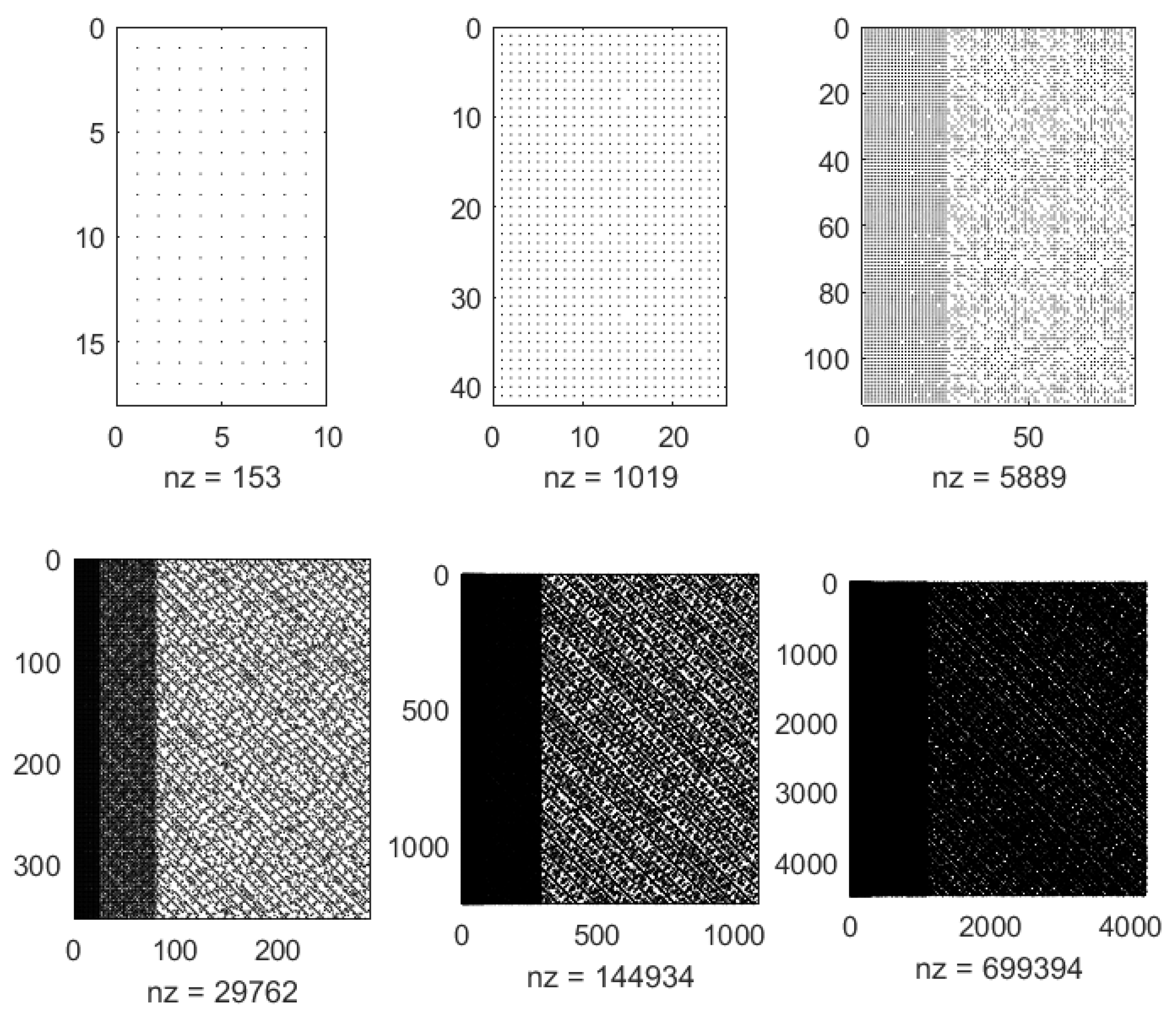
The corresponding RMS-error and observed convergence rates for the H-RBFs method is listed in Table 4. Several observations can be made by looking at Table 4. The H-RBFs interpolation method is numerically stable and has relatively small errors, even for ε = 0.5 case. The RMS-error on 4225 level has been remarkably reduced to 10 6 . Compared with CSRBFs and multilevel interpolation, the present H-RBF method can doubtlessly solve problem (9) with a higher accuracy and lower computational cost. The sparsity behavior of H-RBFs interpolation matrices are displayed in Figure 2.

4. Collocation via H-RBFs

In this section, we discuss the implementation of the H-RBFs collocation method for linear partial differential equations.

4.1. Example 1

We consider the following Poisson problem with Dirichlet boundary conditions,
2 u ( x , y ) = 5 4 π 2 sin ( π x ) cos ( π y 2 ) , ( x , y ) Ω = [ 0 , 1 ] 2 , u ( x , y ) = sin ( π x ) , ( x , y ) Γ 1 , u ( x , y ) = 0 , ( x , y ) Γ 2 ,
where Γ 1 = { ( x , y ) : 0 x 1 , y = 0 } and Γ 2 = Ω Γ 1 . The exact solution of the problem (10) is given by
u ( x , y ) = sin ( π x ) cos ( π y 2 ) .
We use the unsymmetric Kansa method to solve problem (10). At this time, a nonsquare testing is necessary because the small trial space must be tested on a fine-grained space discretization according to Schaback’s theory [21,22]. As always, the interior collocation data are taken to be the same as the centers. We create additional 4 ( N 1 ) equally spaced collocation points for the boundary conditions on each level (red points in Figure 1). That is, on each level, the centers only include blue points, whereas the collocation sites contain blue points in the interior of the domain and red points on the boundary. Consequently, the collocation matrix becomes nonsquare, because the test side has more degrees of freedom than trial side. In our experiments, Wendland’s C 6 function ϕ ( r ) = ( 1 r ) + 8 ( 32 r 3 + 25 r 2 + 8 r + 1 ) is used to construct trial spaces. We list RMS-error and total CPU time (last row in the Tables) for CSRBFs collocation method, multilevel collocation method and H-RBFs collocation method in Table 5, Table 6, Table 7, Table 8, Table 9 and Table 10, respectively.
Table 5 is the nonstationary CSRBFs collocation with fixed scaling parameters of ε = 0.5 and ε = 0.25 . Table 6 is the stationary setting with two different initial parameter values, 0.5 and 0.25 , and then doubles its value for every successive level. We note that the nonconvergence behavior can be observed for the stationary collocation method. Similar observations are reported in detail in Fasshauer’s book [5], where the boundary centers were selected to coincide with the boundary collocation points.
Table 7 and Table 8 are numerical results for multilevel collocation method. Several observations can be made by looking at these two tables. We observe that multilevel collocation method is nonconvergent with some relatively large initial values, such as 0.5 , 0.25 , and 0.125 . With an initial parameter 0.0625 , the method has convergence behavior. However, it seems that the convergence ceases at a later stage. But the multilevel collocation method will have linear convergence if we putting additional centers on boundary. The corresponding numerical experiments have been shown in book [5]. Generally, the bandwidth of the collocation matrix must be allowed to increase slowly from one level to the next (namely, the support radii go slower to zero than the mesh norms) when solving linear partial differential equations by multilevel collocation method. In fact, these phenomena have been noted in Fasshauer’s numerical observations in [23] and theoretical explanations in [16]. Through above experiments (Table 7 and Table 8), the conclusion that we need to add is that the multilevel collocation method is terrible if the centers just being placed in the interior of the domain.
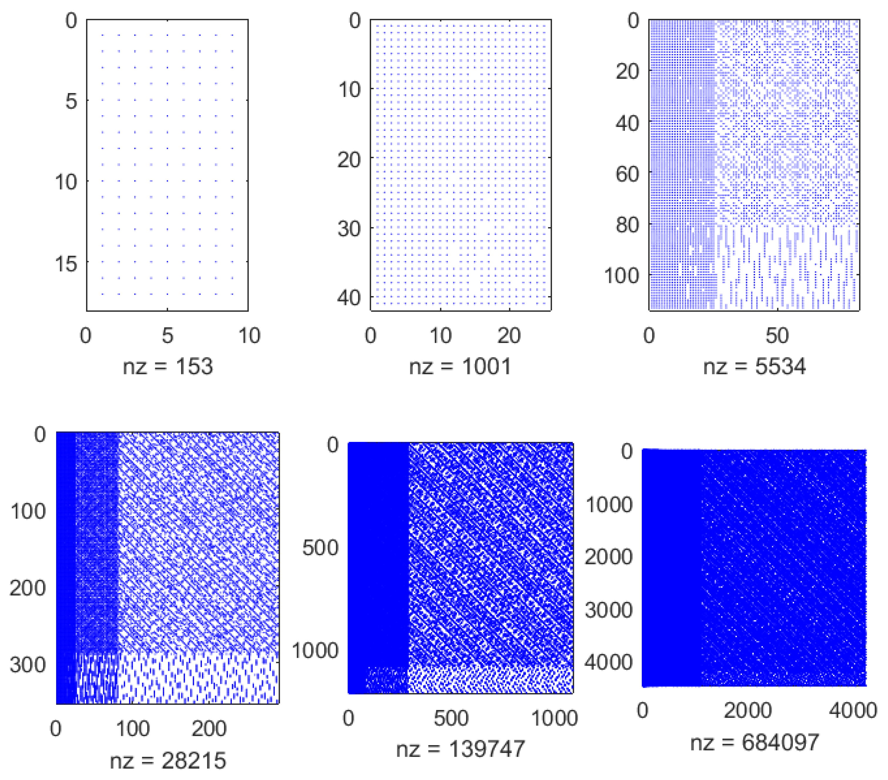
In Table 9 and Table 10, we list RMS-error and CPU time for the hierarchical radial basis functions collocation method. We observe that H-RBFs method has an ideal convergence behavior. Even to a relatively large initial parameter ε = 0.5 , the convergence rate of H-RBFs method is close to 2. With an initial parameter ε = 0.0625 , RMS-error on 4225 level is remarkably reduced to 10 8 , whereas the CPU consumption time is only ~ 37.6 s. Compared with CSRBFs and multilevel collocation method, the present H-RBFs method can solve the model problem with a higher accuracy and lower computational cost. The sparsity behavior of H-RBFs collocation matrices are displayed in Figure 3.

4.2. Example 2

In this subsection, we consider the following Helmholtz test problem,
2 u ( x , y ) + u ( x , y ) = cos ( π x ) cos ( π y ) , ( x , y ) Ω = [ 1 , 1 ] 2 , n u ( x , y ) = 0 , on Ω ,
where n denotes the unit outer normal vector. It is easy to verify that the exact solution for the problem (11) is given by
u ( x , y ) = cos ( π x ) cos ( π y ) 2 π 2 + 1 .
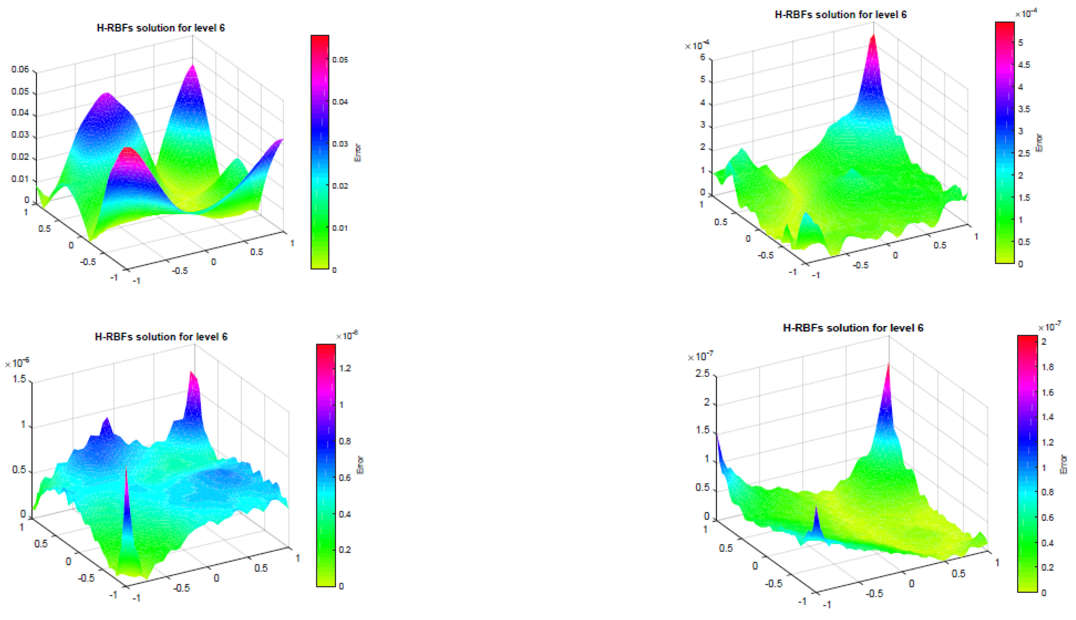
For this example, we use the same centers data, collocation sites, and Wendland’s C 6 function as in Section 4.1. The RMS-error, total CPU time, and observed convergence rates are listed in Table 11 and Table 12, and the sparsity behavior of the H-RBF collocation matrices of this problem are displayed in Figure 4. We observe that it seems that the convergence ceases at a later stage when using a relatively large initial value ε = 0.5 . However, the H-RBF method has ideal convergence behavior and lower computational cost, as in example 1. We also display the plots of the absolute error in Figure 5.

5. Conclusions

To handle the long-standing trade-off principle in the RBF collocation method, we derived hierarchical radial basis functions (H-RBFs) collocation method in the paper. Based on a nested scattered point sets, H-RBF trial spaces are constructed using scaled compactly supported radial basis functions with varying support radii. Several numerical observations were demonstrated in the paper. The experiments showed that H-RBFs collocation method can retain high accuracy with a lower computational cost, when compared with existing CSRBFs collocation method and multilevel RBFs collocation method.
There are many possibilities for enhancement of this method:
(1)
A convergence proof for H-RBFs collocation method will depend on the approximation of H-RBFs trial spaces, new inverse inequality (a frequently used inequality has been given in [24] for RBFs case), and sampling theorem.
(2)
This method can be used for solving well-posed nonlinear partial differential equations, and the convergence analysis of hierarchical radial basis function collocation method for nonlinear discretization will depend on B o ¨ hmer/Schaback theory [25].

Author Contributions

Conceptualization and Formal analysis, Z.L.; Methodology and Writing–original draft preparation, Q.X.

Funding

The research of the first author was partially supported by the Natural Science Foundations of Ningxia Province (No.2019AAC02001), the Natural Science Foundations of China (No.11501313), the Project funded by China Postdoctoral Science Foundation (No.2017M621343), and the Third Batch of Ningxia Youth Talents Supporting Program (No.TJGC2018037). Research of the second author was partially supported by the Natural Science Foundations of Ningxia Province (No.NZ2018AAC03026), and the Fourth Batch of Ningxia Youth Talents Supporting Program.

Acknowledgments

The authors are extremely grateful to Zongmin Wu from Fudan University, and would like to thank two unknown reviewers who made valuable comments on an earlier version of this paper.

Conflicts of Interest

The authors declare no conflicts of interest.

References

  1. Yserentant, H. On the multi-level splitting of finite element spaces. Numer. Math. 1986, 49, 379–412. [Google Scholar] [CrossRef]
  2. Kansa, E.J. Application of Hardy’s multiquadric interpolation to hydrodynamics. In Proceedings of the 1986 Annual Simulations Conference, San Diego, CA, USA, 23 January 1986; Volume 4, pp. 111–117. [Google Scholar]
  3. Schaback, R. Error estimates and condition number for radial basis function interpolation. Adv. Comput. Math. 1995, 3, 251–264. [Google Scholar] [CrossRef]
  4. Fasshauer, G.E.; McCourt, M. Kernel-Based Approximation Mthods Using MATLAB; World Scientific Publishers: Singapore, 2016. [Google Scholar]
  5. Fasshauer, G.E. Meshfree Approximation Methods with MATLAB; World Scientific Publishers: Singapore, 2007. [Google Scholar]
  6. Madych, W.R. Error estimates for interpolation by generalized splines. In Curves and Surfaces; Laurent, P.-J., Le Méhauté, A., Schumaker, L.L., Eds.; Academic Press: New York, NY, USA, 1991; pp. 297–306. [Google Scholar]
  7. Wendland, H. Piecewise polynomial, positive definite and compactly supported radial functions of minimal degree. Adv. Comput. Math. 1995, 4, 389–396. [Google Scholar] [CrossRef]
  8. Wu, Z. Compactly supported positive definite radial functions. Adv. Comput. Math. 1995, 4, 283–292. [Google Scholar] [CrossRef]
  9. Buhmann, M.D. Radial functions on compact support. Proc. Edin. Math. Soc. II 1998, 41, 33–46. [Google Scholar] [CrossRef] [Green Version]
  10. Floater, M.S.; Iske, A. Multistep scattered data interpolation using compactly supported radial basis functions. J. Comput. Applied Math. 1996, 73, 65–78. [Google Scholar] [CrossRef] [Green Version]
  11. Le Gia, Q.T.; Sloan, I.H.; Wendland, H. Multiscale analysis in Sobolev spaces on the sphere. SIAM J. Numer. Anal. 2010, 48, 2065–2090. [Google Scholar] [CrossRef]
  12. Wendland, H. Multiscale analysis in Sobolev spaces on bounded domains. Numer. Math. 2010, 116, 493–517. [Google Scholar] [CrossRef]
  13. Le Gia, Q.T.; Sloan, I.H.; Wendland, H. Multiscale RBF collocation for solving PDEs on spheres. Numer. Math. 2012, 121, 99–125. [Google Scholar] [CrossRef]
  14. Chernih, A.; Le Gia, Q.T. Multiscale methods with compactly supported radial basis functions for Galerkin approximation of elliptic PDEs. IMA J. Numer. Anal. 2014, 34, 569–591. [Google Scholar] [CrossRef]
  15. Chernih, A.; Le Gia, Q.T. Multiscale methods with compactly supported radial basis functions for the Stokes problem on bounded domains. Adv. Comput. Math. 2016, 42, 1187–1208. [Google Scholar] [CrossRef] [Green Version]
  16. Farrell, P.; Wendland, H. RBF multiscale collocation for second order elliptic boundary value problems. SIAM J. Numer. Anal. 2013, 51, 2403–2425. [Google Scholar] [CrossRef]
  17. Le Gia, Q.T.; Sloan, I.H.; Wendland, H. Zooming from global to local: A multiscale RBF approach. Adv. Comput. Math. 2017, 43, 581–606. [Google Scholar] [CrossRef]
  18. Liu, Z. Local multilevel scattered data interpolation. Eng. Anal. Bound. Elem. 2018, 92, 101–107. [Google Scholar] [CrossRef]
  19. Adams, R.A.; Fournier, P. Sobolev Spaces, Pure and Applied Mathematics, 2nd ed.; Academic Press: New York, NY, USA, 2003; Volume 65. [Google Scholar]
  20. Wendland, H. Scattered Data Approximation; Cambridge University Press: Cambridge, UK, 2005. [Google Scholar]
  21. Schaback, R. Convergence of unsymmetric kernel-based meshless collocation methods. SIAM J. Numer. Anal. 2007, 45, 333–351. [Google Scholar] [CrossRef]
  22. Schaback, R. Unsymmetric meshless methods for operator equations. Numer. Math. 2010, 114, 629–651. [Google Scholar] [CrossRef]
  23. Fasshauer, G.E. Solving differential equations with radial basis functions: Multilevel methods and smoothing. Adv. Comput. Math. 1999, 11, 139–159. [Google Scholar] [CrossRef]
  24. Schaback, R.; Wendland, H. Inverse and saturation theroems for radial basis function interpolation. Math. Comput. 2001, 71, 669–681. [Google Scholar] [CrossRef]
  25. Böhmer, K.; Schaback, R. A nonlinear discretization theory. J. Comput. Appl. Math. 2013, 254, 204–219. [Google Scholar] [CrossRef]
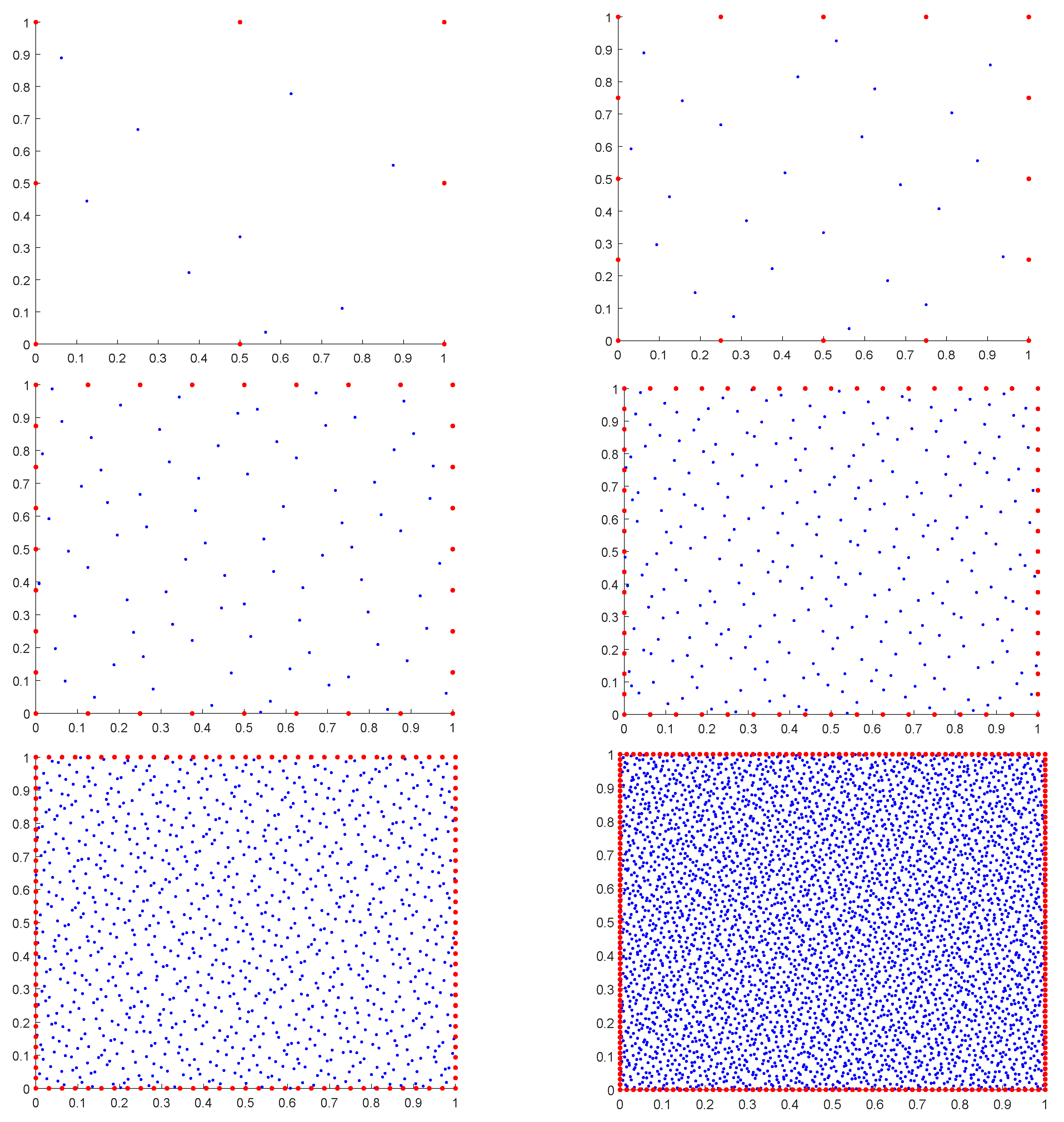
Figure 1. Six scattered data sets used in experiments: N interior Halton points (blue) and 4 ( N 1 ) equally spaced boundary collocation points (red).
Mathematics 07 00964 g001
Figure 2. Sparsity behavior of H-RBF interpolation matrices at level 1, 2, 3, 4, 5, and 6.
Mathematics 07 00964 g002
Figure 3. Possion problem: Sparsity behavior of discrete matrices by H-RBFs collocation at levels 1, 2, 3, 4, 5, and 6.
Mathematics 07 00964 g003
Figure 4. Helmholtz problem: Sparsity behavior of discrete matrices by H-RBFs collocation at levels 1, 2, 3, 4, 5, and 6.
Mathematics 07 00964 g004
Figure 5. Final error graphs on level 6. Top left to bottom right: ε = 0.5, 0.25, 0.125, and 0.0625.
Mathematics 07 00964 g005
Table 1. Compactly supported radial basis function (CSRBF) interpolation: nonstationary.
Centers ε = 0.5 Rate ε = 0.25 Rate
91.113967  × 10 1 1.537637  × 10 1
256.950489  × 10 2 0.6805208.362841  × 10 2 0.878650
817.783806  × 10 3 3.1585678.430085  × 10 3 3.310374
2894.849611  × 10 4 4.0045353.210030  × 10 4 4.714889
10892.253331  × 10 5 4.4277382.115728  × 10 5 3.923360
42251.128459  × 10 6 4.3196343.572115  × 10 6 2.566304
4.42e+01(s) 4.42e+01(s)
Table 2. CSRBF interpolation: stationary.
Centers ε = 0.5 Rate ε = 0.25 Rate
91.113967  × 10 1 1.537637  × 10 1
254.205301  × 10 2 1.4054256.950489  × 10 2 1.145528
812.288906  × 10 2 0.8775519.036469  × 10 3 2.943283
2892.330558  × 10 2 −0.0260185.143627  × 10 3 0.812973
10891.986107  × 10 2 0.2307324.590088  × 10 3 0.164264
42252.010532  × 10 2 −0.0176334.395273  × 10 3 0.062569
1.46e+00(s) 3.16e+00(s)
Table 3. Multilevel interpolation.
CentersInitial
ε = 0.5
RateInitial
ε = 0.25
Rate
91.113967  × 10 1 1.537637  × 10 1
255.321739  × 10 2 1.0657377.271406  × 10 2 1.080408
818.346277  × 10 3 2.6726935.457674  × 10 3 3.735876
2893.142086  × 10 3 1.4094109.231828  × 10 4 2.563598
10891.646392  × 10 3 0.9324142.752895  × 10 4 1.745667
42259.882529  × 10 4 0.7363561.053762  × 10 4 1.385401
2.08e+00(s) 5.53e+00(s)
Table 4. Hierarchical radial basis function (H-RBF) interpolation.
CentersInitial
ε = 0.5
RateInitial
ε = 0.25
Rate
98.715764  × 10 2 9.975067  × 10 2
254.380040  × 10 2 0.9926835.449353  × 10 2 0.872242
818.765413  × 10 3 2.3210502.426089  × 10 2 1.167453
2891.146738  × 10 3 2.9342878.471348  × 10 4 4.839897
10898.960631  × 10 5 3.6777918.592933  × 10 6 6.623297
42259.886575  × 10 6 3.1800581.835490  × 10 6 2.226986
4.42e+00(s) 9.97e+00(s)
Table 5. CSRBFs collocation: nonstationary.
Centers ε = 0.5 Rate ε = 0.25 Rate
95.154990  × 10 1 2.312114  × 10 1
252.523773  × 10 1 1.0303872.501198  × 10 2 3.208521
815.129004  × 10 2 2.2988328.196424  × 10 3 1.609552
2891.169028  × 10 2 2.1333691.976536  × 10 3 2.052021
10899.400882  × 10 4 3.6363702.150290  × 10 4 3.200371
42257.877153  × 10 5 3.5770504.789840  × 10 5 2.166482
5.61e+01(s) 5.59e+01(s)
Table 6. CSRBFs collocation: stationary.
CentersInitial
ε = 0.5
RateInitial
ε = 0.25
Rate
95.154990  × 10 1 2.312114  × 10 1
251.880555  × 10 1 1.4548112.523773  × 10 1 −0.126370
811.845714  × 10 1 0.0269792.415339  × 10 1 0.063357
2893.232111  × 10 1 −0.8082981.619474  × 10 1 0.576701
10894.385499  × 10 1 −0.4402642.008842  × 10 1 −0.310839
42254.782622  × 10 1 −0.1250612.480243  × 10 1 −0.304117
2.11e+00(s) 6.14e+00(s)
Table 7. Multilevel collocation: with initial 0.5 and 0.25.
CentersInitial
ε = 0.5
RateInitial
ε = 0.25
Rate
95.154990  × 10 1 2.312114  × 10 1
255.196034  × 10 1 −0.0114411.827791  × 10 1 0.339111
815.185346  × 10 1 0.0029701.886535  × 10 1 −0.045637
2895.185903  × 10 1 −0.0001551.890747  × 10 1 −0.003218
10895.185993  × 10 1 −0.0000251.891628  × 10 1 −0.000672
42255.186014  × 10 1 −0.0000061.891758  × 10 1 −0.000099
3.19e+00(s) 9.47e+00(s)
Table 8. Multilevel collocation: with initial 0.125 and 0.0625.
CentersInitial
ε = 0.125
RateInitial
ε = 0.0625
Rate
93.345335  × 10 1 2.877511  × 10 1
251.189874  × 10 1 1.4913424.878530  × 10 2 2.560303
811.238221  × 10 1 −0.0574602.944292  × 10 2 0.728526
2891.166663  × 10 1 0.0858811.706502  × 10 2 0.786879
10891.158203  × 10 1 0.0105007.585827  × 10 3 1.169664
42251.159396  × 10 1 −0.0014856.469642  × 10 3 0.229621
2.03e+01(s) 4.21e+01(s)
Table 9. H-RBFs collocation of example 1: with initial 0.5 and 0.25.
CentersInitial
ε = 0.5
RateInitial
ε = 0.25
Rate
95.154990  × 10 1 2.312114  × 10 1
251.200069  × 10 1 2.1028534.838983  × 10 2 2.256436
812.112357  × 10 2 2.5061923.451755  × 10 3 3.809302
2897.398191  × 10 3 1.5136091.075014  × 10 4 5.004903
10892.440784  × 10 3 1.5998285.835322  × 10 6 4.203399
42255.606710  × 10 4 2.1221182.751613  × 10 7 4.406463
4.07e+00(s) 9.69e+00(s)
Table 10. H-RBFs collocation of example 1: with initial 0.125 and 0.0625.
CentersInitial
ε = 0.125
RateInitial
ε = 0.0625
Rate
93.345335  × 10 1 2.877511  × 10 1
251.060521  × 10 2 4.9793056.205372  × 10 3 5.535160
811.898035  × 10 3 2.4821951.655041  × 10 3 1.906651
2892.565084  × 10 5 6.2093572.628040  × 10 5 5.976736
10896.264679  × 10 7 5.3556224.950454  × 10 7 5.730282
42252.553269  × 10 8 4.6168231.102677  × 10 8 5.488478
1.97e+01(s) 3.76e+01(s)
Table 11. H-RBFs collocation of example 2: with initial 0.5 and 0.25.
CentersInitial
ε = 0.5
RateInitial
ε = 0.25
Rate
93.117164  × 10 2 1.719666  × 10 1
252.035525  × 10 2 0.6148338.951139  × 10 2 0.941985
811.837566  × 10 2 0.1476058.238622  × 10 3 3.441596
2891.749727  × 10 2 0.0706663.459194  × 10 3 1.251967
10891.744016  × 10 2 0.0047171.833905  × 10 3 0.915517
42251.787914  × 10 2 −0.0358641.024535  × 10 4 4.161878
1.94e+00(s) 5.48e+00(s)
Table 12. H-RBFs collocation of example 2: with initial 0.125 and 0.0625.
CentersInitial
ε = 0.125
RateInitial
ε = 0.0625
Rate
95.473827  × 10 1 3.289428  × 10 1
251.411404  × 10 2 5.2773476.743427  × 10 2 2.286283
812.332565  × 10 3 2.5971412.429136  × 10 3 4.794967
2894.059524  × 10 4 2.5225352.783964  × 10 4 3.125231
10891.776398  × 10 5 4.5142841.239397  × 10 6 7.811358
42255.102425  × 10 7 5.1216283.532572  × 10 8 5.132776
1.25e+01(s) 2.62e+01(s)