Design of Fuzzy Sampling Plan Using the Birnbaum-Saunders Distribution


1
Department of Mathematics and Statistics, Riphah International University Islamabad, Islamabad 45710, Pakistan
2
Department of Statistics, Faculty of Science, King Abdulaziz University, Jeddah 21551, Saudi Arabia
*
Author to whom correspondence should be addressed.
Mathematics 2019, 7(1), 9; https://doi.org/10.3390/math7010009
Submission received: 18 November 2018
/
Revised: 12 December 2018
/
Accepted: 14 December 2018
/
Published: 21 December 2018
(This article belongs to the Special Issue New Challenges in Neutrosophic Theory and Applications)
Abstract
:Acceptance sampling is one of the essential areas of quality control. In a conventional environment, probability theory is used to study acceptance sampling plans. In some situations, it is not possible to apply conventional techniques due to vagueness in the values emerging from the complexities of processor measurement methods. There are two types of acceptance sampling plans: attribute and variable. One of the important elements in attribute acceptance sampling is the proportion of defective items. In some situations, this proportion is not a precise value, but vague. In this case, it is suitable to apply flexible techniques to study the fuzzy proportion. Fuzzy set theory is used to investigate such concepts. It is observed there is no research available to apply Birnbaum-Saunders distribution in fuzzy acceptance sampling. In this article, it is assumed that the proportion of defective items is fuzzy and follows the Birnbaum-Saunders distribution. A single acceptance sampling plan, based on binomial distribution, is used to design the fuzzy operating characteristic (FOC) curve. Results are illustrated with examples. One real-life example is also presented in the article. The results show the behavior of curves with different combinations of parameters of Birnbaum-Saunders distribution. The novelty of this study is to use the probability distribution function of Birnbaum-Saunders distribution as a proportion of defective items and find the acceptance probability in a fuzzy environment. This is an application of Birnbaum-Saunders distribution in fuzzy acceptance sampling.
1. Introduction
An acceptance sampling plan is used to determine how many units can be selected from a lot, or consignment, and how many defective units are allowed in that sample. If the number of defective units is above the preset number of defective items, the lot is excluded. According to the rule of acceptance sampling, quality can be monitored by checking a few units from the whole lot. The plan that mentions guidelines for sampling and the associated criteria for accepting or rejecting a lot is called the acceptance sampling plan. This acceptance sampling plan can be implemented to check raw material, the material in a process or finished goods. An acceptance sampling plan can be classified as an attribute acceptance sampling plan and a variable acceptance sampling plan. An acceptance sampling plan can be classified with further attributes as a single sampling plan, double sampling plan, multiple sampling plans, and sequential sampling plan. An elementary acceptance sampling plan is a single sampling plan. In a single sampling plan, we select (n) units from the entire lot. This consists of (N) units. After selection of n units they are examined; if the number of damaged units (d) is more than the specified number of defective items (c), the lot will be disallowed. Otherwise, it will be passed. The performance of any acceptance sampling plan can be judged by its operating characteristic (OC) curve. It determines how well an acceptance sampling plan distinguishes between good and bad lots. This OC curve has two parameters (n, c), where n is sample size and c is acceptance number. In an acceptance sampling plan, two groups are involved: the supplier and buyer. The supplier desires to avoid rejection of a good lot (producer’s risk) and the buyer tries to avert acceptance of a bad lot (consumer’s risk). In case a bad lot is accepted, it is the responsibility of the consumer. The producer’s risk is denoted by α. This is the probability of rejection of the lot having an average quality level (AQL). Similarly, the consumer’s risk is denoted with β. This shows the probability of acceptance of the lot, having low quality (LQL) [1]. The proportion of defective items is denoted by p and treated as a precise number. However, in some situations, it is not possible to get the precise numerical value of p. Mostly this value is determined by the expert, based on his judgment. It is used to calculate fuzzy acceptance probability. Further, this fuzzy p value and fuzzy acceptance probability are used to design a fuzzy OC curve [1]. In the study presented in Reference [2], the authors suggested a double acceptance sampling plan, based on assumption that lifetime of the product follows a generalized logistic distribution with known shape parameters, and analyzed the operating characteristic curve to several ratios of the true median life to the specified life. In the study presented in Reference [3], the authors proposed the double sampling plan and specified the design parameters fulfilling both the producer’s and consumer’s risks at the same time for a stated reliability, in the form of the mean ratio to the specific life. Moreover, double sampling and group sampling plans are constructed using the two-point technique, with the assumption that the lifetime of the product follows the Birnbaum-Saunders distribution. In the study presented in Reference [4], the pioneer of fuzzy set theory gave scientific structure to study imprecise and ambiguous concepts that are based on human judgment; comprising verbal expressions, contentment degree and significance degree, that are often fuzzy. A linguistic variable consists of expressions in a natural language, but not the number. In Reference [5] the authors applied fuzzy set theory to help explain complex and not easy to express linguistic terms, in traditional measurable terms. In Reference [6] the authors proposed a single acceptance sampling plan with a fuzzy parameter and explained the single acceptance sampling plan with fuzzy probability theory. In Reference [7] the authors used the expression for the OC curve and various values to help accept or reject a lot for a particular number of defective items. Proficiency of different acceptance sampling plans can be assessed by using the OC curve. These OC curves are used to determine the producer’s risk, as well as the consumer’s risk [8]. In Reference [9] the authors suggested using acceptance sampling in the fuzzy environment using Poisson distribution. In Reference [10] the authors explored if N is large, then the defective items will have a fuzzy binomial distribution. In Reference [11] the authors applied parameters of the acceptance sampling plan, sample size n, and acceptance number c, in a fuzzy environment. Acceptance probabilities of two major discrete distributions were also derived. The multiple deferred sampling plans and characteristic curves were proposed—where (p) proportion of defective items was treated as a fuzzy number—and also proposed fuzzy OC curves with different combinations of parameters [12]. Multiple deferred acceptance sampling plans with inspection errors were proposed by the authors of Reference [13]. In the study presented in Reference [14], the authors investigated the inspection errors and their impact on a single acceptance sampling plan, when the proportion of defective items was not known exactly. In Reference [15] the authors proposed an acceptance sampling plan for geospatial data with uncertainty in the proportion of defective items. In Reference [16] the authors investigated a double acceptance sampling plan with the fuzzy parameter. Average outgoing quality (AOQ) and average total inspection (ATI) in a double acceptance sampling plan with the imprecise proportion of defective items were presented [17]. In Reference [18] the authors suggested the fuzzy parameter for quality interval acceptance sampling plan, applying Poisson distribution. The fuzzy double acceptance sampling plan for Poisson distribution was proposed by the authors in Reference [19]. In Reference [20] the authors proposed an application of Weibull distribution in an acceptance sampling plan in the fuzzy environment and calculated fuzzy acceptance probabilities for different sample sizes using real-life data. In Reference [21] the authors proposed truncated life time, based on the Birnbaum-Saunders (BS) distribution. This distribution is used to define the number of stress cycles until failure of the material. In Reference [22] the authors applied the concept of the failure process of materials due to weariness, to design the BS distribution. Estimation of parameters based on crack length data was proposed in Reference [23]. In Reference [24] the authors presented a literature review of the BS distribution and discussed in detail the importance of this distribution and its application in different fields. In this study [25], they developed an acceptance sampling plan using the BS distribution to get the minimum sample size, n.
The aim of this article was to apply a single acceptance sampling plan when data were fuzzy and the proportion of defective items followed the BS distribution. According to the best of our knowledge, there is no work on the fuzzy plan using the BS distribution in the literature. In this paper, we will develop the fuzzy sampling plan using this distribution. The application of the proposed sampling will be given with the aid of a real example.
2. Materials and Methods
Design of Proposed Plan
Probability distribution function (Pdf) of BS distribution
where α is the shape parameter and λ is the scale parameter, Φ(.) is the standard normal cumulative function and . It can be shown that the median of the BS distribution is equal to the scale parameter and the mean of the BS distribution is
Here we write the assumptions for the BS distribution.
Let be called the termination ratio. The cumulative distribution function (Cdf) given in Equation (5) can be rewritten as
The acceptance probability
According to [26], the acceptance probability of sampling plans can be obtained by using the binomial distribution. The lot acceptance probability of a lot in a single acceptance sampling plan (SASP) case is given as
The proportion of defective items in the fuzzy form.
According to the equation proposed by the authors of Reference [27].
, i = 2, 3, 4 and .
α-cut of
α-cut ofat α = 0
where p is the in Equation (4).
Fuzzy acceptance probability
The fuzzy acceptance probability when the number of defective items, c = 0, and α = 0
The fuzzy acceptance probability based when the number of defective items, c = 1 and α = 0
Here are calculated using CDF of the BS distribution
The design for a single acceptance sampling plan (ASP) to generate a fuzzy operating characteristic curve (FOC)
- Step 1.
- The sample size for a lot is n.
- Step 2.
- Specify the acceptance number (or action limit) c for a sample and the experiment time t0.
- Step 3.
- Perform the experiment for the sample size n and record the number of failures for a sample.
- Step 4.
- Accept the lot if at most c failures are observed in the sample. Truncate the experiment and reject the lot if more than c failures are observed in the sample.
- Step 5.
- Calculation of fuzzy p (proportion of defective items) using Equation (6).
- Step 6.
- Calculation of fuzzy acceptance probability using Equations (10) and (11).
- Step 7.
- Design of fuzzy OC curve (FOC) includes k and the acceptance probability, where k is the transformation of the fuzzy proportion of defective items.
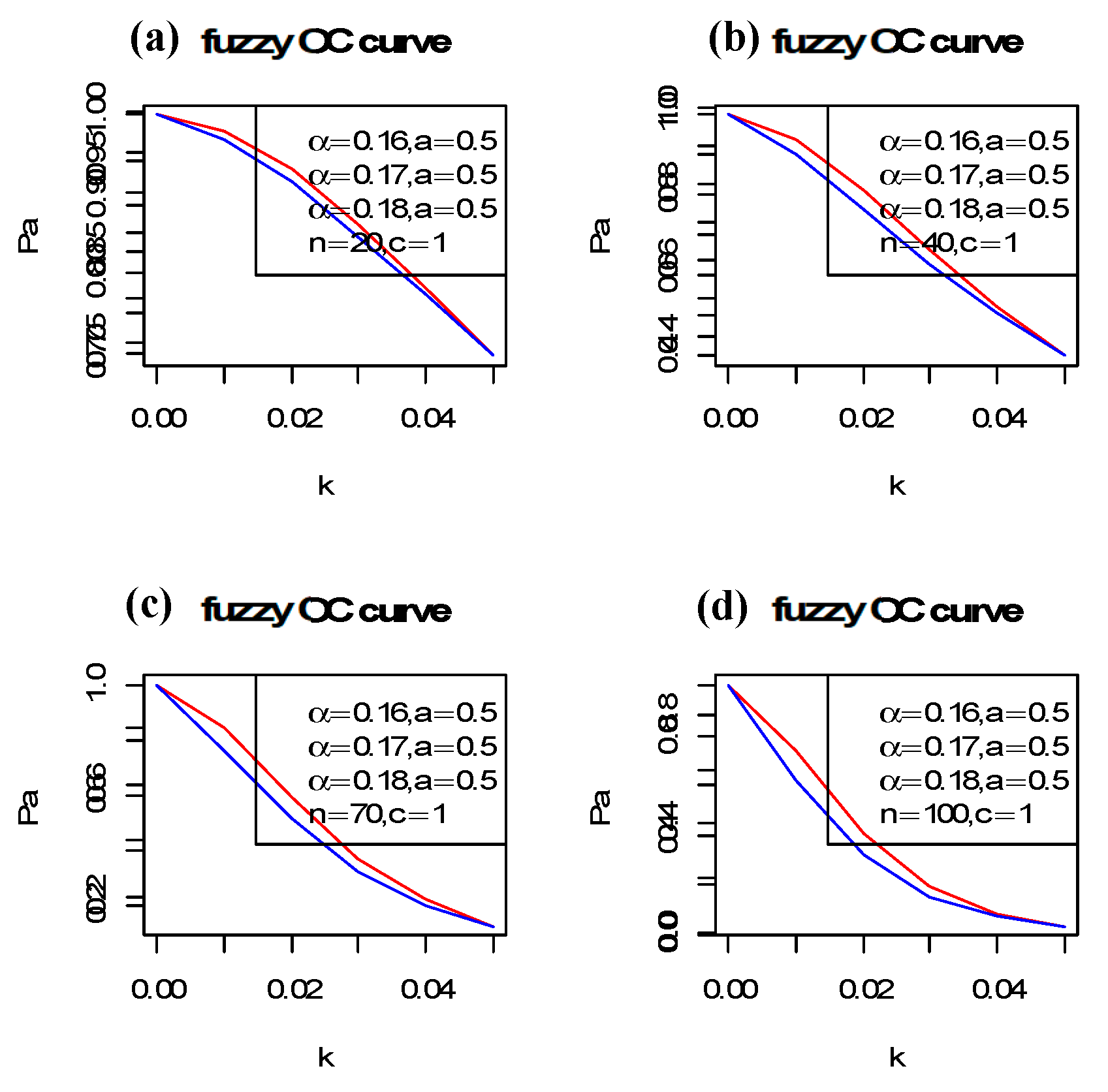
The advantage of the fuzzy OC curve is that it is flexible and can be applied when the proportion of defective items is fuzzy. Secondly, the width of the fuzzy OC curve indicates the quality. Where the wider the width, the lesser the quality, and vice versa. In this study, the width of the fuzzy OC curve is influenced by the mean ratio. When the mean ratio is higher, the width of the band decreases. When the mean ratio is lower, the width increases. The advantage of this approach is that it can be applied to study any fuzzy data, which follows the BS distribution. This approach is more flexible than conventional p because it considers intermediate values of the fuzzy curve.
The fuzzy proportion of defective item k at α = 0 is denoted by and the fuzzy acceptance probability as . Values for sample size n = 5 and acceptance number c = 0, will therefore be (0.00, 0.001), and (0.95, 0.96), respectively at k = 0.01. Similarly, values of proportion and acceptance probability for sample size n = 5 and acceptance number c = 0, will be (0.052, 0.054) and (0.77, 0.78), respectively at k = 0.01. Furthermore, the fuzzy proportion of defective item k at α = 0 is denoted by and the fuzzy acceptance probability as . These values for sample size n = 5 and acceptance number c = 1, will be the proportion of defective items (0.01, 0.029), and the acceptance probability (0.99, 0.995) at K = 0.01.
3. Real Life Example
In this section, we will discuss the application of the proposed sampling plan using real data selected from [28] and [29]. As mentioned above, the BS distribution is also known as the fatigue life distribution. It is used extensively in reliability applications to model failure times. The BS distribution is used in circumstances where occurring of events is independent of each other, from one cycle to another cycle, with same random distribution [29]. In this study, the failure life data given in Reference [28] is used. The authors of Reference [28] found that the data follow the BS distribution. The fatigue life data of aluminum coupons having n = 101 observations are shown in Table 1.
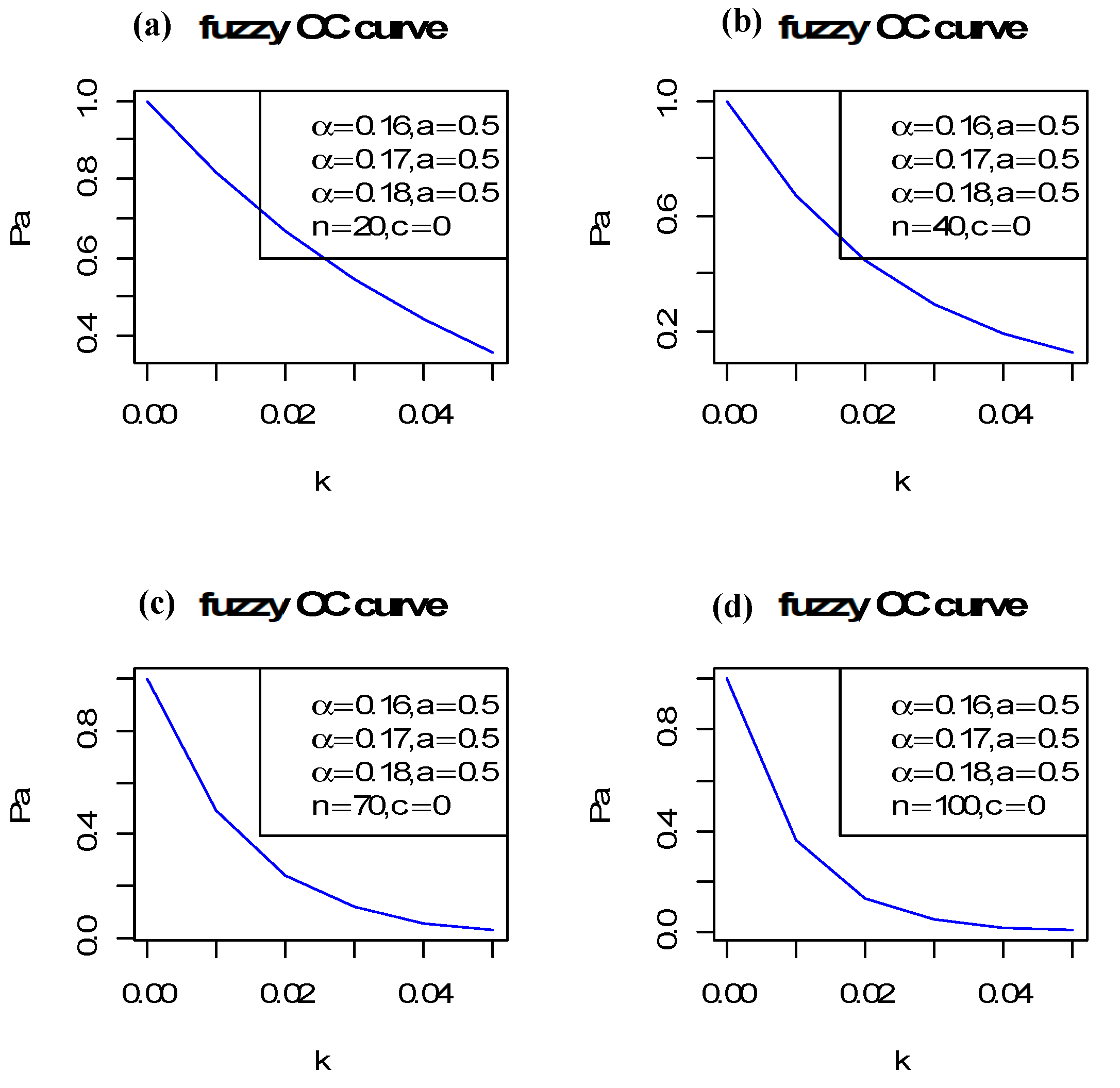
We assume that data follows the BS distribution, the proportion of defective items p is fuzzy and the shape parameter is taken as the trapezoidal fuzzy number, = (0.15, 0.16, 0.17, 0.18). When the actual mean is , the termination ratio a = 0.5 is then truncated, time will be t = 67 for c = 0, and at , the proportion of defective items is .0211673. The acceptance probabilities are calculated by using Equations (9) and (10), for different sample sizes n = (5,25,75,100) and K = (0.0, 0.01,0.02, 0.03, 0.04, 0.05). The fuzzy OC curve is designed using fuzzy p values and fuzzy acceptance probabilities for c = 0. Similarly, when , termination ratio a = 0.67 is then truncated, time will be t = 89.7 for c = 1. In this case, acceptance number c = 1, and = 1, = 0.01923. The acceptance probabilities are calculated using Equation (11) for different sample sizes n = (5,25,75,100) and K = (0.0, 0.01, 0.02, 0.03, 0.04, 0.05). The fuzzy OC curve is developed using p values and acceptance probabilities for c = 1. Fuzzy acceptance probability for Birnbaum-Saunders distribution is presented in Table 2 and Table 3 using real life data and their respective fuzzy OC curves are shown in Figure 1, Figure 2 and Figure 3. Entire calculations and graphs were completed using R software and codes were given in Appendix A. Acceptance probability is influenced by mean ratio, when mean ratio increases it reduces Uuncertainty and bandwidth of fuzzy OC curve become narrow while decreasing mean ration increases the width of fuzzy OC curve. The fuzzy OC curves show more convexity when sample size n increases. Fuzzy OC curve with c = 0 shows less uncertainty than c = 1. We presented acceptance probabilities and fuzzy OC curves with c = 0, it is almost equal to conventional OC curve. The fuzzy OC curve for c = 0 and c = 1 is more convex at large sample size as compared to small sample size.
4. Conclusions
Acceptance sampling is one of the important aspects of statistical quality control. When the data follow the Birnbaum-Saunders distribution and the proportion of defective items is fuzzy, acceptance probability and the OC curve can be presented in a fuzzy form. In this article, the fuzzy OC curve of the Birnbaum-Saunders distribution is presented in a single acceptance sampling plan, using the binomial distribution. The fuzzy OC curve has a band with two bounds, lower and upper. The width of the band depends upon the uncertainty in the proportion of defective items in the fuzzy environment. Less uncertainty will give a narrow width. The fuzzy OC curves also show more convexity at a large sample size. The mean ratio in the Birnbaum-Saunders distribution is another important factor in quality. Here, a lower value of the mean ratio causes the width of the band of the fuzzy OC curve to increase. This indicates more uncertainty. The advantage of this approach is that it can be used to calculate the proportion of defective items when fuzzy data follows a Birnbaum-Saunders distribution, because mostly we assume the value of the proportion of defective items without using any distribution. Secondly, the fuzzy acceptance probability based on the Birnbaum-Saunders distribution is calculated. The fuzzy OC curve of the Birnbaum-Saunders distribution is constructed based on fuzzy p and the acceptance probability. The OC curve is more convex at large sample sizes, as compared to small sample sizes. It was concluded that when data followed the Birnbaum-Saunders distribution, this proposed approach was suitable to calculate the proportion (p), the acceptance probability, and the OC curve in both conventional and fuzzy form. In the future, we will apply the same concept to group acceptance sampling and chain acceptance sampling in a fuzzy environment.
Author Contributions
Conceptualization, M.F.K. and M.Z.K.; methodology, M.Z.K.; software, M.A.; validation, A.R.M.
Funding
This research received no funding.
Acknowledgments
The authors are deeply thankful to the reviewers and editor for their valuable suggestions to improve the quality of the paper.
Conflicts of Interest
The authors declare that there is no conflict of interest regarding the publication of this paper.
Abbreviations
| OC | operating characteristic |
| OC curve | operating characteristic curve |
| (FOC) curve | fuzzy operating characteristic curve |
| AQL | average quality level |
| LQL | low quality level |
| probability density function. | |
| cdf | Cumulative distribution function |
| SASP | single acceptance sampling plan |
| BS | Birnbaum-Saunders |
Appendix A
R codes
- #When n = 5, 20, 30, 30, c = 0
- rm(list=ls ())
- windows ()
- par(mfrow=c(2,2))
- a = 0.5 #For c = 0 at t = 67
- alpha = c(0.15, 0.16, 0.17, 0.18)
- K = seq(0, 0.05, 0.01)
- x = a*((1 + alpha^2)/2) #Here b is teated as Alpha
- y = 0.5# 1, 2, 3, 4, 5, 6 values of ratio of
- X = c((1/alpha)*(sqrt(x/y)−sqrt(y/x)))
- FX = pnorm(X, mean = 0, sd = 1, lower.tail = TRUE, log.p = FALSE)
- FX
- p = FX
- p = 2.470246e-16
- K = seq(0,0.05,0.01)
- W = p + K
- p = 0.226627400
- W = p + K
- #p = 0.226627400
- p = 0.019
- W = p + K
- K = seq(0,0.05,0.01)
- c = o, a = 0.5) and (c = 1 when a = 0.67) for a = 0.5, p = 2.470246e-16, for a = 0.67 p = 0.01923
- B = dbinom(0,10,K) # B = (1−K)^5 When n = 5, c = 0 (1)
- A = dbinom(0,10, W)# A = (1−(K+p))^5#When n = 5, c = 0 (2)
- data.frame(A,B)
- data.frame(K,W,A,B)
- #B = (1-K)^5 # THIS WILL GIVE US UPPER BAND HIGHER PROBABILITY
- #A = (1-(K+p))^5#THIS WILL GIVE US LOWER BAND LOWER PROBABILITY
- plot(K,A,type = “l”, col = “red”, xlab = “K”, ylab = “Pa “, main = “fuzzy OC curve”)
- par(new = TRUE)
- plot(W,B,type = “l”, col = “blue”, xlab = “k”, ylab = “ “, main = ““)
- legend(“topright”,c(expression(paste(alpha==0.15,”,”,a==0.67)),expression(paste(alpha==0.16,”,”,a==0.67)),expression(paste(alpha==0.17,”,”,a==0.1)),expression(paste(alpha==0.18,”,”,a==0.67)),expression(paste(n==5,”,”,c==0))))
References
- Kahraman, C.; Kaya, İ. Fuzzy acceptance sampling plans. In Production Engineering and Management under Fuzziness; Springer: Heidelberg, Germany, 2010; pp. 457–481. [Google Scholar]
- Aslam, M.; Jun, C.-H. A double acceptance sampling plan for generalized log-logistic distributions with known shape parameters. J. Appl. Stat. 2010, 37, 405–414. [Google Scholar] [CrossRef]
- Aslam, M.; Jun, C.-H.; Ahmad, M. New acceptance sampling plans based on life tests for Birnbaum–Saunders distributions. J. Stat. Comput. Simul. 2011, 81, 461–470. [Google Scholar] [CrossRef]
- Zadeh, L.A. Information and control. Fuzzy Sets 1965, 8, 338–353. [Google Scholar]
- Zimmermann, H.J. Fuzzy Set Theory and Its Applications; Kluwer Academic Publishers: Dordrecht, The Netherlands, 1991. [Google Scholar]
- Sadeghpour Gildeh, B.; Jamkhaneh, E.B.; Yari, G. Acceptance single sampling plan with fuzzy parameter. Iran. J. Fuzzy Syst. 2011, 8, 47–55. [Google Scholar]
- Grzegorzewski, P. Acceptance sampling plans by attributes with fuzzy risks and quality levels. In Frontiers in Statistical Quality Control; Springer: Heidelberg, Germany, 2001; pp. 36–46. [Google Scholar]
- Montgomery, D.C. Ihntroduction to Statistical Quality Control; John Wiley & Sons: New York, NY, USA, 2009. [Google Scholar]
- Jamkhaneh, E.B.; Sadeghpour-Gildeh, B.; Yari, G. Acceptance single sampling plan with fuzzy parameter with the using of poisson distribution. World Acad. Sci. Eng. Technol. 2009, 3, 1–20. [Google Scholar]
- Buckley, J.J. Fuzzy Probability and Statistics; Springer: Heidelberg, Germany, 2006. [Google Scholar]
- Turanoğlu, E.; Kaya, İ.; Kahraman, C. Fuzzy acceptance sampling and characteristic curves. Int. J. Comput. Intell. Syst. 2012, 5, 13–29. [Google Scholar] [CrossRef]
- Afshari, R.; Gildeh, B.S.; Sarmad, M. Multiple Deferred State Sampling Plan with Fuzzy Parameter. Int. J. Fuzzy Syst. 2017, 20, 549–557. [Google Scholar] [CrossRef]
- Afshari, R.; Gildeh, B.S.; Sarmad, M. Fuzzy multiple deferred state attribute sampling plan in the presence of inspection errors. J. Intell. Fuzzy Syst. 2017, 33, 503–514. [Google Scholar] [CrossRef]
- Jamkhaneh, E.B.; Sadeghpour-Gildeh, B.; Yari, G. Inspection error and its effects on single sampling plans with fuzzy parameters. Struct. Multidiscip. Optim. 2011, 43, 555–560. [Google Scholar] [CrossRef]
- Tong, X.; Wang, Z. Fuzzy acceptance sampling plans for inspection of geospatial data with ambiguity in quality characteristics. Comput. Geosci. 2012, 48, 256–266. [Google Scholar] [CrossRef]
- Sadeghpour-Gildeh, B.; Yari, G.; Jamkhaneh, E.B. Acceptance double sampling plan with fuzzy parameter. Available online: http://citeseerx.ist.psu.edu/viewdoc/download?doi=10.1.1.864.8328&rep=rep1&type=pdf (accessed on 1 November 2018).
- Jamkhaneh, E.B.; Gildeh, B.S. Notice of Retraction AOQ and ATI for Double Sampling Plan with Using Fuzzy Binomial Distribution. In Proceedings of the International Conference on Intelligent Computing and Cognitive Informatics (ICICCI), Kuala Lumpur, Malaysia, 22–23 June 2010. [Google Scholar]
- Divya, P. Quality interval acceptance single sampling plan with fuzzy parameter using poisson distribution. Int. J. Adv. Res. Technol. 2012, 1, 115–125. [Google Scholar]
- Jamkhaneh, E.B.; Gildeh, B.S. Acceptance Double Sampling Plan using Fuzzy Poisson Distribution. World Appl. Sci. J. 2012, 15, 1692–1702. [Google Scholar]
- Venkatesh, A.; Subramani, G. Acceptance sampling for the secretion of Gastrin using crisp and fuzzy Weibull distribution. Int. J. Eng. Res. Appl. 2014, 4, 564–569. [Google Scholar]
- Wu, C.-J.; Tsai, T.-R. Acceptance sampling plans for Birnbaum-Saunders distribution under truncated life tests. Int. J. Reliab. Qual. Saf. Eng. 2005, 12, 507–519. [Google Scholar] [CrossRef]
- Birnbaum, Z.W.; Saunders, S.C. A new family of life distributions. J. Appl. Probab. 1969, 6, 319–327. [Google Scholar] [CrossRef] [Green Version]
- Birnbaum, Z.W.; Saunders, S.C. Estimation for a family of life distributions with applications to fatigue. J. Appl. Probab. 1969, 6, 328–347. [Google Scholar] [CrossRef]
- Balakrishnan, N.; Kundu, D. Birnbaum-Saunders Distribution: A Review of Models, Analysis and Applications. arXiv, 2018; arXiv:1805.06730. [Google Scholar]
- Balakrishnan, N.; Leiva, V.; Lopez, J. Acceptance sampling plans from truncated life tests based on the generalized Birnbaum–Saunders distribution. Commun. Stat. Simul. Comput. 2007, 36, 643–656. [Google Scholar] [CrossRef]
- Stephens, K.S. The Handbook of Applied Acceptance Sampling: Plans, Principles, and Procedures; Asq Press: Milwaukee, WI, USA, 2001. [Google Scholar]
- Jamkhaneh, E.B.; Gildeh, B.S. Chain sampling plan using Fuzzy probability theory. J. Appl. Sci. 2011, 11, 3830–3838. [Google Scholar] [CrossRef]
- From, S.G.; Li, L. Estimation of the parameters of the Birnbaum–Saunders distribution. Commun. Stat. Theory Methods 2006, 35, 2157–2169. [Google Scholar] [CrossRef]
- Croarkin, C.; Tobias, P.; Zey, C. Engineering Statistics Handbook; NIST: Gaithersburg, MD, USA, 2002.
Figure 1.
The fuzzy operating characteristic (OC) Curve of the Birnbaum-Saunders distribution at c = 0 (a) n = 20, (b) n = 40, (c) n = 70, and (d) n = 100.
Figure 1.
The fuzzy operating characteristic (OC) Curve of the Birnbaum-Saunders distribution at c = 0 (a) n = 20, (b) n = 40, (c) n = 70, and (d) n = 100.

Figure 2.
The fuzzy operating characteristic (OC) curve of Birnbaum-Saunders distribution at c = 1, mean ratio = 0.5, (a) n = 20, (b) n = 40, (c) n = 70, and (d) n = 100.
Figure 2.
The fuzzy operating characteristic (OC) curve of Birnbaum-Saunders distribution at c = 1, mean ratio = 0.5, (a) n = 20, (b) n = 40, (c) n = 70, and (d) n = 100.

Figure 3.
The fuzzy operating characteristic (OC) curve of Birnbaum-Saunders distribution at c = 1, mean ratio = 0.5, (a) n = 5, (b) n = 15, (c) n = 30, and (d) n = 50.
Figure 3.
The fuzzy operating characteristic (OC) curve of Birnbaum-Saunders distribution at c = 1, mean ratio = 0.5, (a) n = 5, (b) n = 15, (c) n = 30, and (d) n = 50.


Table 1.
Fatigue data of aluminum in hours.
| 70 | 90 | 96 | 97 | 99 | 100 | 103 | 104 | 104 | 105 | 107 | 108 | 108 | 108 | 109 |
| 109 | 112 | 112 | 113 | 114 | 114 | 114 | 116 | 119 | 120 | 120 | 120 | 121 | 121 | 123 |
| 124 | 124 | 124 | 124 | 124 | 128 | 128 | 129 | 129 | 130 | 130 | 130 | 131 | 131 | 131 |
| 131 | 131 | 132 | 132 | 132 | 133 | 134 | 134 | 134 | 134 | 134 | 136 | 136 | 137 | 138 |
| 138 | 138 | 139 | 139 | 141 | 141 | 142 | 142 | 142 | 142 | 142 | 142 | 144 | 144 | 145 |
| 146 | 148 | 148 | 149 | 151 | 151 | 152 | 155 | 156 | 157 | 157 | 157 | 157 | 158 | 159 |
| 162 | 163 | 163 | 164 | 166 | 166 | 168 | 170 | 174 | 196 | 212. |
Table 2.
Fatigue life data of aluminum coupons.
| K | |||||
|---|---|---|---|---|---|
| 0.00 | [0.00, 0.001] | [0.98, 1.00] | [0.99, 1.00] | [0.99, 1.00] | [0.996, 1.00] |
| 0.01 | [0.01, 0.011] | [0.95, 0.96] | [0.81, 0.82] | [0.73, 0.76] | [0.604, 0.620] |
| 0.02 | [0.02, 0.022] | [0.93, 0.94] | [0.65, 0.66] | [0.53, 0.54] | [0.3640, 0.372] |
| 0.03 | [0.03, 0.041] | [0.85, 0.86] | [0.53, 0.54] | [0.40, 0.43] | [0.213, 0.219] |
| 0.04 | [0.04, 0.051] | [0.81, 0.83] | [0.41, 0.43] | [0.29, 0.31] | [0.125, 0.129] |
| 0.05 | [0.052, 0.054] | [0.77, 0.78] | [0.35, 0.36] | [0.21, 0.23] | [0.076, 0.077] |
Table 3.
The fuzzy acceptance probability of Birnbaum-Saunders distribution for c = 0.
| K | |||||
|---|---|---|---|---|---|
| 0.00 | [0.00, 0.019] | [1.000, 1.00] | [1.0000, 1.00] | [1.00, 1.00] | [0.99, 1.00] |
| 0.01 | [0.01, 0.029] | [0.99, 0.995] | [0.979, 0.97] | [0.827, 0.82] | [0.82, 0.82] |
| 0.02 | [0.02, 0.039] | [0.94, 0.96] | [0.99, 0.949] | [0.55, 0.556] | [0.65, 0.660] |
| 0.03 | [0.03, 0.077] | [0.93, 0.95] | [0.82, 0.826] | [0.338, 0.338] | [0.63, 0.54] |
| 0.04 | [0.04, 0.050] | [0.91, 0.92] | [0.73, 0.730] | [0.190, 0.190] | 0.44, 0.42] |
| 0.05 | [0.05, 0.067] | [0.89, 0.900] | [0.720, 0.7202] | [0.160, 0.160] | [0.35, 0.37] |
© 2018 by the authors. Licensee MDPI, Basel, Switzerland. This article is an open access article distributed under the terms and conditions of the Creative Commons Attribution (CC BY) license (http://creativecommons.org/licenses/by/4.0/).
Share and Cite
MDPI and ACS Style
Khan, M.Z.; Khan, M.F.; Aslam, M.; Mughal, A.R. Design of Fuzzy Sampling Plan Using the Birnbaum-Saunders Distribution. Mathematics 2019, 7, 9. https://doi.org/10.3390/math7010009
AMA Style
Khan MZ, Khan MF, Aslam M, Mughal AR. Design of Fuzzy Sampling Plan Using the Birnbaum-Saunders Distribution. Mathematics. 2019; 7(1):9. https://doi.org/10.3390/math7010009
Chicago/Turabian StyleKhan, Muhammad Zahir, Muhammad Farid Khan, Muhammad Aslam, and Abdur Razzaque Mughal. 2019. "Design of Fuzzy Sampling Plan Using the Birnbaum-Saunders Distribution" Mathematics 7, no. 1: 9. https://doi.org/10.3390/math7010009
Note that from the first issue of 2016, this journal uses article numbers instead of page numbers. See further details here.