Global Dynamics of Leslie-Gower Competitive Systems in the Plane

Abstract

Global dynamic results are obtained for families of competitive systems of difference equations of the form $x_{n+1}=\frac{b_1{x}_n}{{\alpha }_1+x_n+c_1{y}_n},y_{n+1}=\frac{b_2{y}_n}{{\alpha }_2+c_2{x}_n+y_n}n=0,1,\dots ,$ where the parameters $b_1,b_2$ are positive numbers, and ${\alpha }_1,{\alpha }_2,c_1,$ and $c_2$ and the initial conditions $x_0$ and $y_0$ are arbitrary non-negative numbers, when one or both of ${\alpha }_i,i=1,2$ equalls 0. We assume that the denominators of both equations are always positive. We will show that the presence of more parameters will create more dynamic scenarios.

1. Introduction

The system of difference equations,

$$x_{n+1}=\frac{b_1{x}_n}{{\alpha }_1+x_n+c_1{y}_n},y_{n+1}=\frac{b_2{y}_n}{{\alpha }_2+c_2{x}_n+y_n}n=0,1,\dots ,$$

(1)

where the parameters $b_1,b_2$ are positive real numbers, and ${\alpha }_1,{\alpha }_2,c_1,$ and $c_2$ and the initial conditions $x_0$ and $y_0$ are arbitrary non-negative numbers, is considered as a major discrete model that describes the competition of two species, see [1,2,3,4,5,6,7]. In this paper we consider the effect of terms ${\alpha }_1,{\alpha }_2$ on the global dynamics of system (1). The global dynamics of (1) was considered in the case where the parameters ${\alpha }_1,{\alpha }_2$ are positive in [1,2,3,5] and the complete description of the dynamics was given in [5] where the following result was obtained:

Assuming, without loss of generality, that ${\alpha }_1={\alpha }_2=1$, it has been shown in [1] that under the condition $b_1>1$ and $b_2>1$, the points

$$E_0(0,0),E_x(b_1-1,0),E_y(0,b_2-1)$$

are equilibria of Equation (1), and that for some values of the parameters there exists an additional equilibrium point $E_3$ located in the open positive quadrant, given by

$$E\left(\frac{b_2-1}{c_1{c}_2-1}\left(c_1-\frac{b_1-1}{b_2-1}\right),\frac{b_1-1}{c_1{c}_2-1}\left(c_2-\frac{b_2-1}{b_1-1}\right)\right).$$

(2)

Important subsets of parameter space are described in

Table 1. Global behavior of solutions to Equation (1) when $b_1>1$ and $b_2>1$. Equality relations are not represented for the sake of a simpler description.

Condition	${\mathit{c}}_1({\mathit{b}}_2-1)<{\mathit{b}}_1-1$	${\mathit{c}}_1({\mathit{b}}_2-1)>{\mathit{b}}_1-1$
$c_2(b_1-1)<b_2-1$	Case 1. $E_0$ is a repeller $E_x$ is a saddle $E_y$ is a saddle E is an interior local attractor.	Case 2. $E_0$ is a repeller $E_x$ is a saddle $E_y$ attractor on $[0,\infty )\times (0,\infty )$ No interior fixed point exists.
$c_2(b_1-1)>b_2-1$	Case 3. $E_0$ is a repeller $E_x$ is attractor on $(0,\infty )\times [0,\infty )$ $E_y$ is a saddle No interior fixed point exists.	Case 4. $E_0$ is a repeller $E_x$ is a local attractor $E_y$ is a local attractor E is an interior saddle.

, together with corresponding behavior of equilibrium solutions established in [1].

Theorem 4.1 in [5] applies when parameters vary from Case 1 to Case 4 of Table 1. Set

$$\mathcal{A}=\{a\in {\mathbb{R}}_{+}^4:a=(b_1,b_2,c_1,c_2)\mathrm{and}{c}_1(b_2-1)>b_1-1>0\}$$

and define $T_a$ to be the map of Equation (1) restricted to $\mathcal{R}=[0,\infty )\times (0,\infty )$, that is,

$$T_a(x,y)=\left(\frac{b_{1}x}{1+x+c_{1}y},\frac{b_{2}y}{1+c_{2}x+y}\right).$$

Therefore, Theorem 4.1 in [5] gives global behavior of solutions to system (1) on $\mathcal{R}=[0,\infty )\times (0,\infty )$ for $a\in \mathcal{A}$. In particular, a bifurcation occurs when the equilibrium E changes its local character from a locally stable equilibrium to a saddle point. This happens when the parameters cross the critical surface $\mathsf{\Gamma }(b_1,b_2,c_1,c_2)=c_2(b_1-1)-b_2+1=0$.

It is also shown in [1] that the open, positive semiaxis $(0,\infty )\times \left\{0\right\}$ is attracted to $E_x$, and that the open, positive semiaxis $\left\{0\right\}\times (0,\infty )$ is attracted to $E_y$. The following two results describe the global dynamics of system (1) in all cases. The first result gives the global dynamics in the hyperbolic case and the second result in the non-hyperbolic case.

Theorem 1.

Consider system (1).

(i) 

Suppose that $c_1(b_2-1)>b_1-1>0$. If $c_2(b_1-1)>b_2-1$, then $E_y$ is globally asymptotically stable on $[0,\infty )\times (0,\infty )$, and $E_x$ attracts all points on the open semiaxis $(0,\infty )\times \left\{0\right\}$. If $c_2(b_1-1)<b_2-1$, then the stable manifold $W^s\left(E\right)$ in $[0,\infty )\times [0,\infty )$ is the graph of a continuous, increasing function of the first coordinate. Furthermore, a solution $\left\{{\mathbf{x}}_n\right\}$ converges to $E_x$ whenever ${\mathbf{x}}_0$ is above $W^s\left(E\right)$ in South-east ordering, and $\left\{{\mathbf{x}}_n\right\}$ converges to $E_y$ whenever ${\mathbf{x}}_0$ is below $W^s\left(E\right)$ in South-east ordering.

(ii) 

Suppose that $c_1(b_2-1)<b_1-1>0$. If $c_2(b_1-1)>b_2-1$, then $E_x$ is globally asymptotically stable on $[0,\infty )\times (0,\infty )$, and $E_y$ attracts all points on the open semiaxis $\left\{0\right\}\times (0,\infty )$. If $c_2(b_1-1)<b_2-1$, then E is globally asymptotically stable on $(0,\infty )\times (0,\infty )$, $E_y$ attracts all points on the open semiaxis $\left\{0\right\}\times (0,\infty )$, and $E_x$ attracts all points on the open semiaxis $(0,\infty )\times \left\{0\right\}$.

See Figure 1 for graphical interpretation.

The non-hyperbolic case when

$$c_1(b_2-1)=b_1-1\mathrm{and}{c}_2(b_1-1)=b_2-1$$

(3)

was not considered in [1]. When (3) holds, a direct calculation gives that the fixed points of $T_a$ are $E_0(0,0)$ and all points on the segment $\mathcal{E}:=\{E_t:0\le t\le 1\}$, where

$$E_t:=\left((b_1-1)(1-t),(b_2-1)t\right),0\le t\le 1.$$

The eigenvalues of the Jacobian of $T_a$ at $E_t$ are

$${\lambda }_1=1\mathrm{and}{\lambda }_2=(1-t)\frac{1}{b_1}+t\frac{1}{b_2},0\le t\le 1,$$

and corresponding eigenvectors are

$${\mathbf{e}}_1=\left(-\frac{1-b_1}{1-b_2},1\right)\mathrm{and}{\mathbf{e}}_2=\left(b_2{(1-b_1)}^2(1-t),b_1{(1-b_2)}^{2}t\right),0\le t\le 1.$$

It is shown in [8] that, for system (1), the hypotheses of Theorem 5 in [6] are satisfied and that all solutions fall inside an invariant rectangular region. Therefore, every solution of (1) converges to an equilibrium point. A direct calculation shows that the origin is a repeller. We conclude that every nonzero solution converges to a point $(\overline{x},\overline{y})\in \mathcal{E}$. Also, with an argument similar to the one used in [9], one has that the equilibrium depends continuously on the initial condition. That is, if $T^{*}(x,y):=\lim T_a^n(x,y)$, then $T^{*}$ is continuous. These observations, together with an application of Theorem 1 in [6] lead to the following result.

Theorem 2.

Assume (3) holds. Then,

(i) 

Every nonzero solution to system (1) converges to an equlibrium $(\overline{x},\overline{y})\in \mathcal{E}$.

(ii) 

For every $(\overline{x},\overline{y})\in \mathcal{E}$ with $\overline{x}\ne 0$ and $\overline{y}\ne 0$, the stable set $W_{(\overline{x},\overline{y})}^s$ is an unbounded, increasing curve $\mathcal{C}$ with endpoint $(0,0)$.

(iii) 

The limiting equilibrium varies continuously with the initial condition.

See Figure 1 for graphical interpretation.

Statement (ii) excludes equilibria of the form $(0,\overline{y})$ and $(\overline{x},0)$ since the hypotheses of Theorem 1 in [6] are not satisfied at these points.

In this paper, we consider two related systems, namely

$$x_{n+1}=\frac{b_1{x}_n}{x_n+c_1{y}_n},y_{n+1}=\frac{b_2{y}_n}{c_2{x}_n+y_n}n=0,1,\dots$$

(4)

and

$$x_{n+1}=\frac{b_1{x}_n}{{\alpha }_1+x_n+c_1{y}_n},y_{n+1}=\frac{b_2{y}_n}{c_2{x}_n+y_n}n=0,1,\dots ,$$

(5)

where all present coefficients are positive and the initial conditions are non-negative and such that $x_0+y_0>0$. We derive the global dynamics of both systems (4) and (5), which explains the effect of the coefficients ${\alpha }_1,{\alpha }_2$ on the global dynamics. Related systems are considered in [2,3,10,11,12].

The paper is organized as follows. Section 2 presents some basic preliminary results about competitive systems, which is our main tool in proving the results. Section 3 contains the global dynamics of system (4) and Section 4 gives the global dynamics of system (5). Actually we show that the global dynamics of all three systems is determined by their linearized dynamics. We use different techniques to prove the results for systems (4) and (5). In particular, we will use the fact that system (4) is homogeneous to obtain the exact equation of the global stable manifold of positive equilibrium solution of system (4). We will show that the presence of more parameters will create more dynamic scenarios in such a way that system (1) exhibits one additional dynamic scenario compared to system (5) which in turn will have one additional dynamic scenario more than system (4). This is in contrast with the global dynamics of second order difference equation

$$x_{n+1}=\frac{\alpha +\beta x_n+\gamma x_{n-1}}{A+B{x}_n+C{x}_{n-1}}.n=0,1,\dots ,$$

with all non-negative parameters and initial conditions such that $A+B{x}_n+C{x}_{n-1}>0,n=0,1,\dots$, where the most complicated dynamics occurs in the special case of Lyness’ equation when $\gamma =A=B=0$ [13]. We will also show that systems (1) and (4) are solvable for the special values of parameters while there is not a formula for the exact solution of system (5) at this time for any choice of parameters.

2. Preliminaries

In this section we provide some basic facts about competitive maps and systems of difference equations in the plane.

Definition 1.

Let R be a subset of ${\mathbb{R}}^2$ with nonempty interior, and let $T:R\to R$ be a map (i.e., a continuous function). Set $T(x,y)=\left(f\right(x,y),g(x,y\left)\right)$. The map T is competitive if $f(x,y)$ is non-decreasing in x and non-increasing in y, and $g(x,y)$ is non-increasing in x and non-decreasing in y. If both f and g are non-decreasing in x and y, we say that T is cooperative. If T is competitive (cooperative), the associated system of difference equations

$$\left\{\begin{array}{ccc}\hfill x_{n+1}& =& f(x_n,y_n)\hfill \\ \hfill y_{n+1}& =& g(x_n,y_n)\hfill \end{array}\right.,n=0,1,2,\dots ,(x_{-1},x_0)\in R$$

(6)

is said to be competitive (cooperative). The map T and associated difference equations system are said to be strongly competitive (strongly cooperative) if the adjectives non-decreasing and non-increasing are replaced by increasing and decreasing.

If T is differentiable, a sufficient condition for T to be strongly competitive is that the Jacobian matrix of T at any $x\in R$ has the sign configuration

$$\left(\begin{array}{cc}+& -\\ -& +\end{array}\right).$$

Competitive systems of the form (6) have been studied by many authors such as Clark, Hess, Hirsch and Smith, Kulenović, Merino, Nurkanović, Leonard and May, Selgrade, Smale, Smith [4,6,7,14,15,16,17,18,19] and others. In [1,2] the authors gave an interesting applications of this theory to some basic models in population dynamics. Many open problems and conjectures about the dynamics of competitive systems of linear fractional difference equations are gien in [8].

Denote with ${⪯}_{se}$ the South-East partial order in the plane whose non-negative cone is the standard fourth quadrant $\left\{\right(x,y):x\ge 0,y\le 0\}$, that is, $(x^1,y^1)⪯(x^2,y^2)$ if and only if $x^1\le x^2$ and $y^1\ge y^2$. The North-East partial order ${⪯}_{ne}$ is defined analogously with the non-negative cone given by the standard first quadrant $\left\{\right(x,y):x\ge 0,y\ge 0\}$.

Competitive maps T in the plane preserve the South-East ordering: $T\left(\mathbf{u}\right){⪯}_{se}T\left(\mathbf{v}\right)$ whenever $\mathbf{u}{⪯}_{se}\mathbf{v}$. Similarly, cooperative maps in the plane preserve the North-East ordering. In fact, the concepts of competitive and cooperative (for maps) may be defined in terms of the order preserving properties of the maps. Thus the theory of competitive maps is a special case of the theory of order preserving maps (or monotone operators).

Order preserving maps in ${\mathbb{R}}^n$, and in particular competitive maps in ${\mathbb{R}}^2$, may have chaotic dynamics. Smale [19] showed that any continuous time vector field on the standard $(n-1)$-simplex in ${\mathbb{R}}^n$ can be embedded on a smooth, competitive vector field in ${\mathbb{R}}^n$ for which the simplex is an attractor. In the case of a planar system (6), this means that any first order difference equation, including chaotic, can be embedded into a competitive system (6) in the plane. An effective method to do this is provided by Smith in [7].

Let ⪯ be a partial order on ${\mathbb{R}}^n$ with non-negative cone P. For $x,y\in {\mathbb{R}}^n$ the order interval $〚x,y〛$ is the set of all z such that $x⪯z⪯y$. We say $x\prec y$ if $x⪯y$ and $x\ne y$, and $x\ll y$ if $y-x\in P^{\circ }$, where $P^{\circ }$ is the interior of P. A map T on a subset of ${\mathbb{R}}^n$ is order preserving if $T\left(x\right)⪯T\left(y\right)$ whenever $x\prec y$, strictly order preserving if $T\left(x\right)\prec T\left(y\right)$ whenever $x\prec y$, and strongly order preserving if $T\left(x\right)\ll T\left(y\right)$ whenever $x\prec y$.

Let $T:R\to R$ be a map with a fixed point $\overline{x}$ and let $R^{\prime }$ be an invariant subset of R that contains $\overline{x}$. We say that $\overline{x}$ is stable (asymptotically stable) relative to $R^{\prime }$ if $\overline{x}$ is a stable (asymptotically stable) fixed point of the restriction of T to $R^{\prime }$.

Definition 2.

Let $\mathcal{S}$ be a nonempty subset of ${\mathbb{R}}^2$. A competitive map $T:\mathcal{S}\to \mathcal{S}$ is said to satisfy condition ($O+$) if for every x, y in $\mathcal{S}$, $T\left(x\right){⪯}_{ne}T\left(y\right)$ implies $x{⪯}_{ne}y$, and T is said to satisfy condition ($O-$) if for every x, y in $\mathcal{S}$, $T\left(x\right){⪯}_{ne}T\left(y\right)$ implies $y{⪯}_{ne}x$.

The following theorem was proved by deMottoni-Schiaffino for the Poincaré map of a periodic competitive Lotka-Volterra system of differential equations. Smith generalized the proof to competitive and cooperative maps [20,21].

Theorem 3.

Let $\mathcal{S}$ be a nonempty subset of ${\mathbb{R}}^2$. If T is a competitive map for which ($O+$) holds then for all $x\in \mathcal{S}$, $\left\{T^n\left(x\right)\right\}$ is eventually componentwise monotone. If the orbit of x has compact closure, then it converges to a fixed point of T. If instead ($O-$) holds, then for all $x\in \mathcal{S}$, $\left\{T^{2n}\right\}$ is eventually componentwise monotone. If the orbit of x has compact closure in $\mathcal{S}$, then its omega limit set is either a period-two orbit or a fixed point.

System (5) is an example of what might happen if the orbit of x has no compact closure in $\mathcal{S}$. The next two results are stated for order-preserving maps on ${\mathbb{R}}^n$. These results are known but are given here for completeness. See Theorem 2.1 in [5] and Corollary 1 in [5]. See [15] for a more general version that is valid in ordered Banach spaces.

Theorem 4.

For a nonempty set $R\subset {\mathbb{R}}^n$ and ⪯ a partial order on ${\mathbb{R}}^n$, let $T:R\to R$ be an order preserving map, and let $a,b\in R$ be such that $a\prec b$ and $〚a,b〛\subset R$. If $a⪯T\left(a\right)$ and $T\left(b\right)⪯b$, then $〚a,b〛$ is invariant and

i. 

There exists a fixed point of T in $〚a,b〛$.

ii. 

If T is strongly order preserving, then there exists a fixed point in $〚a,b〛$ which is stable relative to $〚a,b〛$.

iii. 

If there is only one fixed point in $〚a,b〛$, then it is a global attractor in $〚a,b〛$ and therefore asymptotically stable relative to $〚a,b〛$.

Corollary 1.

If the non-negative cone of ⪯ is a generalized quadrant in ${\mathbb{R}}^n$, and if T has no fixed points in $〚u_1,u_2〛$ other than $u_1$ and $u_2$, then the interior of $〚u_1,u_2〛$ is either a subset of the basin of attraction of $u_1$ or a subset of the basin of attraction of $u_2$.

Our main tool will be results from [4,5,6] regarding the existence of the global stable and unstable manifolds of competitive maps in the plane.

The non-hyperbolic equilibrium solution of system (6) is said to be of stable (resp. unstable) type if the second eigenvalue of the Jacobian matrix evaluated at the equilibrium solution is by absolute value less than 1 (resp. bigger than 1).

3. Global Dynamics of System (4)

First we give some basic results about the global behavior of system (4). Denote by

$$T(x,y)=\left(\frac{b_{1}x}{x+c_{1}y},\frac{b_{2}y}{c_{2}x+y}\right),$$

the map associated with system (4). System (4) is homogeneous and was partially investigated in [22].

Lemma 1.

(a) 

Every solution of system (4) satisfies $x_n\le b_1,y_n\le b_2,n\ge 1$.

(b) 

$\det J_T(x,y)=0$ for every $(x,y)$, where $J_T$ denotes the Jacobian matrix of the map T.

(c) 

$T(x_0,0)=E_x(b_1,0)$, $T(0,y_0)=E_y(0,b_2)$ for every $x_0>0,y_0>0$.

(d) 

Every solution of system (4) satisfies the difference equation

$$r_{n+1}=\frac{b_2}{b_1}{r}_n\frac{1+c_1{r}_n}{c_2+r_n},n\ge 0,$$

where $r_n=y_n/x_n$.

(e) 

If

$$(b_2-b_1{c}_2)(b_1-b_2{c}_1)>0,$$

(7)

then the map T has an invariant line

$${\ell }_S:y=\frac{b_2-b_1{c}_2}{b_1-b_2{c}_1}x.$$

(8)

Proof. 

The Jacobian matrix $J_T$ of the map T has the form

$$J_T(x,y)=\left(\begin{array}{cc}\frac{b_1{c}_{1}y}{{(x+c_{1}y)}^2}& -\frac{b_1{c}_{1}x}{{(x+c_{1}y)}^2}\\ -\frac{b_2{c}_{2}y}{{(c_{2}x+y)}^2}& \frac{b_2{c}_{2}x}{{(c_{2}x+y)}^2}\end{array}\right),$$

(9)

which implies (b). Parts (a) and (c) follow by immediate checking. Part (d) follows by dividing equations of system (4). Part (e) follows from (d) since $\frac{b_2-b_1{c}_2}{b_1-b_2{c}_1}$ is exactly an equilibrium of the equation in (d). □

System (4) always has two equilibrium solutions on the axes, $E_x(b_1,0)$, $E_y(0,b_2)$. It can also have either exactly one interior equilibrium solution E or an infinite number of equilibrium solutions $E_t$. Since the interior equilibrium solution E is an intersection of two equilibrium curves (isoclines) ${\mathcal{C}}_1:x+c_{1}y=b_1,{\mathcal{C}}_2:c_{2}x+y=b_2$ it will exist if either $\frac{b_2}{c_2}<b_1,\frac{b_1}{c_1}<b_2$ (x-intercept of ${\mathcal{C}}_2$ smaller than x-intercept of ${\mathcal{C}}_1$ and y-intercept of ${\mathcal{C}}_2$ bigger than y-intercept of ${\mathcal{C}}_1$) or $\frac{b_2}{c_2}>b_1,\frac{b_1}{c_1}>b_2$ (x-intercept of ${\mathcal{C}}_1$ smaller than x-intercept of ${\mathcal{C}}_2$ and y-intercept of ${\mathcal{C}}_1$ bigger than y-intercept of ${\mathcal{C}}_2$). These two geometrical conditions can be unified as condition (7).

Condition (7) implies that $c_1{c}_2\ne 1$, in which case the interior equilibrium $E(\overline{x},\overline{y})$ is given as:

$$\overline{x}=\frac{b_1-b_2{c}_1}{1-c_1{c}_2},\overline{y}=\frac{b_2-b_1{c}_2}{1-c_1{c}_2}.$$

(10)

Notice that $b_2<b_1{c}_2$, $b_1<b_2{c}_1$ implies $c_1{c}_2>1$ and $b_2>b_1{c}_2$, $b_1>b_2{c}_1$ implies $c_1{c}_2<1$. If either $(b_2-b_1{c}_2)(b_1-b_2{c}_1)<0$, $b_2=b_1{c}_2$ and $b_1\ne b_2{c}_1$, or $b_1=b_2{c}_1$ and $b_2\ne b_1{c}_2$ then there are no interior equilibrium points. Furthermore, if $b_2=b_1{c}_2$ and $b_1=b_2{c}_1$, the two equilibrium curves ${\mathcal{C}}_1,{\mathcal{C}}_2$ coincide and every point on the segment $x+c_{1}y=b_1,x,y\ge 0$ is an equilibrium solution $E_t(b_1-c_{1}t,t),t\in [0,b_2]$. See

Table 2. The equilibrium points of system (4).

Condition	Equilibrium Points
$(b_2-b_1{c}_2)(b_1-b_2{c}_1)<0$, $b_2=b_1{c}_2 \mathrm{and} b_1\ne b_2{c}_1,$ $\mathrm{or} b_2\ne b_1{c}_2\mathrm{and}{b}_1=b_2{c}_1$	$E_x,E_y$
$(b_2-b_1{c}_2)(b_1-b_2{c}_1)>0$	$E_x,E_y,E$
$b_2=b_1{c}_2 \mathrm{and} b_1=b_2{c}_1$	$E_x,E_y,E_t$

summarizing the equilibrium points of system (4).

The following result describes the local stability character of all equilibrium solutions.

Lemma 2.

Consider system (4).

(a) 

The equilibrium solution $E_x$ is locally asymptotically stable if $b_2<b_1{c}_2$, non-hyperbolic of stable type if $b_2=b_1{c}_2$ and a saddle point if $b_2>b_1{c}_2$. In each case, the eigenvectors associated with the eigenvalues ${\lambda }_1=0$ and ${\lambda }_2=\frac{b_2}{b_1{c}_2}$ are ${\mathbf{e}}_1=(1,0)$ and ${\mathbf{e}}_2=(-\frac{b_1{c}_1{c}_2}{b_2},1)$.

(b) 

The equilibrium solution $E_y$ is locally asymptotically stable if $b_1<b_2{c}_1$, non-hyperbolic of stable type if $b_1=b_2{c}_1$ and a saddle point if $b_1>b_2{c}_1$. In each case, the eigenvectors associated with the eigenvalues ${\lambda }_1=0$ and ${\lambda }_2=\frac{b_1}{b_2{c}_1}$ are ${\mathbf{e}}_1=(0,1)$ and ${\mathbf{e}}_2=(\frac{b_1}{c_1{c}_2{b}_2},-1)$.

(c) 

The interior equilibrium solution E is a saddle point when $b_2<b_1{c}_2$ and $b_1<b_2{c}_1$ and is locally asymptotically stable when $b_2>b_1{c}_2$ and $b_1>b_2{c}_1$.

(d) 

The interior equilibrium solutions $E_t$ are non-hyperbolic of the stable type and the eigenvector which corresponds to ${\lambda }_1=0$ is given as ${\mathbf{e}}_1=(1,y)$.

Proof. 

(a)

In view of (9), we have

$$J_T\left(E_x\right)=\left(\begin{array}{cc}0& -c_1\\ 0& \frac{b_2}{b_1{c}_2}\end{array}\right),$$

which implies that the eigenvalues of the Jacobian matrix are ${\lambda }_1=0,{\lambda }_2=\frac{b_2}{b_1{c}_2}$. The corresponding eigenvectors are as stated.

(b)

In view of (9), we have

$$J_T\left(E_y\right)=\left(\begin{array}{cc}\frac{b_1}{b_2{c}_1}& 0\\ -c_2& 0\end{array}\right),$$

which implies that the eigenvalues of the Jacobian matrix are ${\lambda }_1=0,{\lambda }_2=\frac{b_1}{b_2{c}_1}$. The corresponding eigenvectors are as stated.

(c)

The eigenvalues of the Jacobian matrix evaluated at the equilibrium E, ${\lambda }_1=0$ and ${\lambda }_2=\mathrm{Tr}\left(J_T\left(E\right)\right)$, correspond to the roots of the characteristic polynomial $p\left(t\right)=t^2-\mathrm{Tr}\left(J_T\left(E\right)\right)t$. Note that ${\lambda }_2>0$ by (9). Furthermore

$$p\left(1\right)=\frac{(b_1-b_2{c}_1)(b_2-b_1{c}_2)}{b_1{b}_2(1-c_1{c}_2)}\mathrm{and}{p}^{\prime }\left(1\right)=\frac{b_2(b_1-b_2{c}_1)+b_1(b_2-b_1{c}_2)}{b_1{b}_2(1-c_1{c}_2)}.$$

(11)

Consequently, if $b_2<b_1{c}_2$ and $b_1<b_2{c}_1$ then $p\left(1\right)<0$ and $p^{\prime }\left(1\right)>0$ and if $b_2>b_1{c}_2$ and $b_1>b_2{c}_1$ then $p\left(1\right)>0$ and $p^{\prime }\left(1\right)>0$. It follows that E is a saddle point when $b_2<b_1{c}_2$ and $b_1<b_2{c}_1$ and is locally asymptotically stable when $b_2>b_1{c}_2$ and $b_1>b_2{c}_1$.

(d)

In this case, the eigenvalues of the Jacobian matrix evaluated at the equilibrium $E_t$ are ${\lambda }_1=0,{\lambda }_2=1$. The eigenvector that corresponds to ${\lambda }_1=0$ is ${\mathbf{e}}_1=(1,y)$, where $y>0$ satisfies $x+c_{1}y=b_1$ and points towards the first quadrant.

□

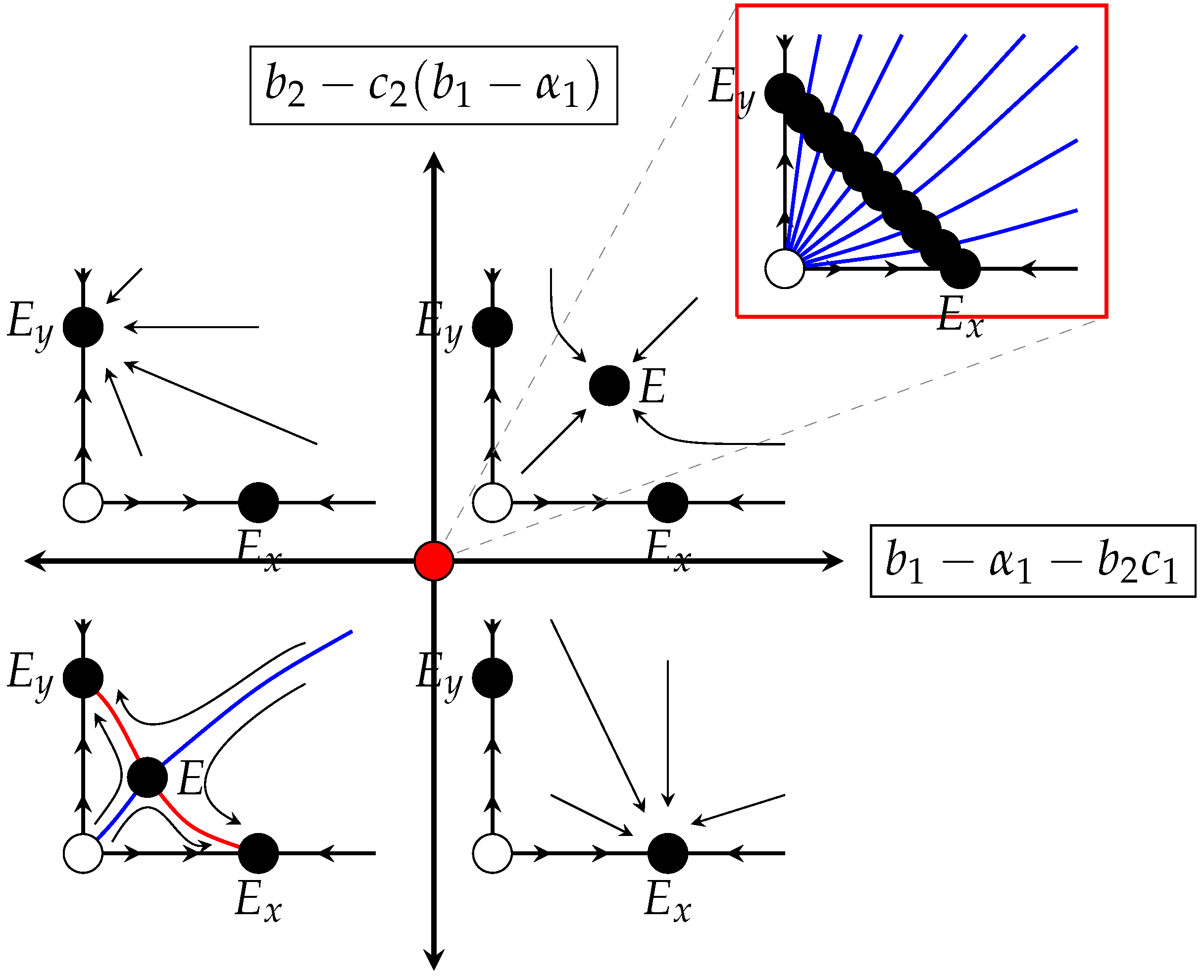
Now, global behavior of system (4) is described by the following result:

Theorem 5.

Consider system (4).

(a) 

If $b_2<b_1{c}_2,b_1<b_2{c}_1$, then the equilibrium solutions $E_x,E_y$ are locally asymptotically stable and the interior equilibrium E is a saddle point. The separatrix ${\ell }_S$, which is a graph of a continuous, non-decreasing curve, is the basin of attraction of E and the region below (resp. above) ${\ell }_S$ is the basin of attraction of $E_x$ (resp. $E_y$).

(b) 

If $b_2>b_1{c}_2,b_1>b_2{c}_1$, then the equilibrium solutions $E_x,E_y$ are saddle points and the interior equilibrium E is locally asymptotically stable. Every solution in the first quadrant which starts off the coordinate axes converges to E. Every solution which starts on the positive part of the x-axis (resp. y-axis) is attracted by $E_x$ (resp. $E_y$).

(c) 

If $b_2<b_1{c}_2,b_1>b_2{c}_1$ (resp. $b_2>b_1{c}_2,b_1<b_2{c}_1$), then the equilibrium solution $E_x$ (resp. $E_y$) is locally asymptotically stable and $E_y$ (resp. $E_x$) is a saddle point. The basin of attraction of $E_x$ (resp. $E_y$) is the first quadrant of initial conditions without the positive part of the y-axis (resp. x-axis), which is attracted by $E_y$ (resp. $E_x$).

(d) 

If $b_1=b_2{c}_1$ and $b_2=b_1{c}_2$, then there is an infinite family of equilibrium solutions $E_t,t\in [0,b_2]$ for which there exists the global stable manifold ${\mathcal{W}}^s\left(E_t\right)$, which is the graph of a continuous, non-decreasing function asymptotic to $(0,0)$ and is exactly the basin of attraction of $E_t$. The limiting equilibrium varies continuously with the initial condition.

(e) 

If $E_x$ (resp. $E_y$) is non-hyperbolic and $E_y$ (resp. $E_x$) is locally asymptotically stable then $E_y$ (resp. $E_x$) attracts the first quadrant of initial conditions except the positive part of x-axis (resp. y-axis) which is attracted by $E_x$ (resp. $E_y$). If $E_x$ (resp. $E_y$) is non-hyperbolic and $E_y$ (resp. $E_x$) is a saddle point then $E_x$ (resp. $E_y$) attracts the first quadrant of initial conditions except the positive part of y-axis (resp. x-axis) which is attracted by $E_y$ (resp. $E_x$).

See Figure 2 for graphical interpretation.

Proof. 

(a)

First we show that T does not have any period-two solutions. Our condition implies $c_1{c}_2>1$. By direct calculation one can show that a period-two solution satisfies the equation

$$b_1{c}_2(c_1{c}_2-1)x^2+(b_1+b_2{c}_1)(b_1{c}_2-b_2)x+b_1{b}_2(b_1+b_2{c}_1)=0.$$

Please note that

$$D=(b_1+b_2{c}_1)(b_2+b_1{c}_2)(b_1{c}_2(b_1-b_2{c}_1)+b_2{c}_1(b_2-b_1{c}_2)-b_1{b}_2(c_1{c}_2-1))<0,$$

which means that both terms of such solution are complex conjugate and so there is no period-two solution in the first quadrant.

Taking into account that the Jacobian matrix evaluated at E has all non-zero entries, Theorem 5 of [4] implies the existence and uniqueness of both global stable and unstable manifolds ${\mathcal{W}}^s\left(E\right)$ and ${\mathcal{W}}^u\left(E\right)$ and so ${\mathcal{W}}^s\left(E\right)={\ell }_S$. Furthermore, Theorem 5 of [4] implies that every $(x_0,y_0)$ below ${\ell }_S$ will satisfy $T^n\left((x_0,y_0)\right)\in \left[[E,E_x]\right]$ for some $n\ge N$. In view of Corollary 1, $T^n\left((x_0,y_0)\right)\to E_x$. In a similar way, we can treat the case when $(x_0,y_0)$ is above ${\ell }_S$.

(b)

In view of Lemma 2 part (a), the eigenvectors which correspond to $E_x$ and $E_y$ point to the interior of the fourth and the second quadrant, which means that the local unstable manifolds ${\mathcal{W}}_{loc}^u\left(E_x\right)$ and ${\mathcal{W}}_{loc}^u\left(E_y\right)$ exist and point strictly toward E. Thus there exist points $u,v$ in the interior of $〚E_y,E_x〛$, arbitrarily close to $E_y$ and $E_x$ such that $u{⪯}_{se}T\left(u\right){⪯}_{se}E{⪯}_{se}T\left(v\right){⪯}_{se}v$. Now, statement iii of Theorem 3 implies that E is a global attractor in $\left[\right[u,v\left]\right]$, which completes the proof.

(c)

Assume that $b_2<b_1{c}_2,b_1>b_2{c}_1$ which implies that $E_x$ is locally asymptotically stable and $E_y$ is a saddle point. In view of Lemma 2 part (b), the eigenvector which corresponds to $E_y$ points to the interior of the fourth quadrant, which means that the local unstable manifold ${\mathcal{W}}_{loc}^u\left(E_y\right)$ exists and points strictly toward $E_x$. Thus there exists a point u in the interior of $〚E_y,E_x〛$, arbitrarily close to $E_y$ such that $u{⪯}_{se}T\left(u\right)$. However, then this shows that the map T has a lower solution in every neighborhood of $E_y$, which in view of Theorem 6 in [6] implies that the interior of $〚E_y,E_x〛$ is a subset of the basin of attraction of $E_x$. The result follows.

The proof when $b_2>b_1{c}_2,b_1<b_2{c}_1$ is similar and will be omitted.

(d)

By Theorem 1 of [6], for each $E_t$ there exists the set ${\mathcal{W}}^s\left(E_t\right)$ passing through $E_t$ and asymptotic to $(0,0)$, which is the graph of a continuous, non-decreasing function, which is exactly the basin of attraction of $E_t$. The continuity of the limiting equilibrium solution as a function of initial conditions follows as in [9].

(e)

The proof is similar to the proof of part (c) and will be omitted.

□

Remark 1.

In the special case $c_1=c_2=1$ system (4) has an explicit solution. Indeed in this case we have that $\frac{y_{n+1}}{x_{n+1}}=B\frac{y_n}{x_n}$, where $B=\frac{b_2}{b_1}$ and so the solution of system (4) is

$$x_n=\frac{b_1{x}_0}{x_0+y_0{B}^{n-1}},y_n=\frac{b_1{y}_0{B}^n}{x_0+y_0{B}^{n-1}},n=0,1,\dots .$$

Thus $B<1$ implies $(x_n,y_n)\to (b_1,0),n\to \infty$ and $B>1$ implies $(x_n,y_n)\to (0,b_2),n\to \infty$ while $B=1$ implies $(x_n,y_n)=(\frac{b_1{x}_0}{x_0+y_0},\frac{b_1{y}_0}{x_0+y_0}),n=0,1,\dots$, which is simplified version of possible competitive scenarios, where the first two are competitive exclusion and the third is competitive coexistence.

In the special case $c_1=c_2=1,{\alpha }_1={\alpha }_2>0$ system (1) is solvable, although the solution formula is complicated. Using this formula one can similarly explained competitive coexistence and competitive exclusion scenarios.

4. Global Dynamics of System (5)

In this section, we present the global behavior of system (5). Denote by

$$\tilde{T}(x,y)=\left(\frac{b_{1}x}{{\alpha }_1+x+c_{1}y},\frac{b_{2}y}{c_{2}x+y}\right),$$

the map associated with system (5).

Lemma 3.

(a) 

Every solution of system (5) satisfies $x_n<b_1,y_n\le b_2,n\ge 1$;

(b) 

$\tilde{T}(x,y)$ satisfies ($O+$) condition on ${(0,\infty )}^2$ and so T has no period-two points;

(c) 

For every $y_0>0$, $\tilde{T}(0,y_0)=(0,b_2)$;

(d) 

For every $x_0>0$, ${\tilde{T}}^n(x_0,0)=\left({\displaystyle \frac{b_1-{\alpha }_1}{1-{\left(\frac{{\alpha }_1}{b_1}\right)}^n}},0\right)$.

Proof. 

Part (a) and (c) follow by immediate checking and part (d) follows by solving the resulting Beverton-Holt one-dimensional equation. Notice

$$\tilde{T}\left(\begin{array}{c}{x}_1\\ y_1\end{array}\right){⪯}_{ne}\tilde{T}\left(\begin{array}{c}{x}_2\\ y_2\end{array}\right)\iff \left(\begin{array}{c}\frac{b_1{x}_1}{{\alpha }_1+x_1+c_1{y}_1}\\ \frac{b_2{y}_1}{c_2{x}_1+y_1}\end{array}\right){⪯}_{ne}\left(\begin{array}{c}\frac{b_1{x}_2}{{\alpha }_1+x_2+c_1{y}_2}\\ \frac{b_2{y}_2}{c_2{x}_2+y_2}\end{array}\right).$$

This is equivalent to

$${\alpha }_1(x_1-x_2)\le c_1(x_2{y}_1-x_1{y}_2),x_2{y}_1-x_1{y}_2\le 0.$$

This implies that $x_1\le x_2$ and $x_2{y}_1\le x_1{y}_2$ and thus $x_1\le x_2,y_1\le y_2$, that is $(x_1,y_1){⪯}_{ne}(x_2,y_2)$. □

Please note that a direct consequence of the above form of $J_{\tilde{T}}(x,y)$ is that $\tilde{T}$ is strongly competitive. This will play a pivotal role in the global behavior of the system.

System (5) always has an equilibrium solution on the y-axis, $E_y(0,b_2)$. Provided that ${\alpha }_1<b_1$, there exists an equilibrium solution on the x-axis, $E_x(b_1-{\alpha }_1,0)$. Depending on the values of the parameters ${\alpha }_1,b_1,b_2,c_1$ and $c_2$, there is also the possibility of either exactly one interior equilibrium solution E or an infinite number of interior equilibrium solutions $E_t$. The interior equilibrium solution is an intersection of two equilibrium curves ${\mathcal{C}}_1:{\alpha }_1+x+c_{1}y=b_1$ and ${\mathcal{C}}_2:c_{2}x+y=b_2$. This solution will exist if either $\frac{b_2}{c_2}<b_1-{\alpha }_1$ and $b_2>\frac{b_1-{\alpha }_1}{c_1}$ (i.e., the x-intercept of ${\mathcal{C}}_2$ is smaller than the x-intercept of ${\mathcal{C}}_1$ and the y-intercept of ${\mathcal{C}}_2$ is bigger than the y-intercept of ${\mathcal{C}}_1$) or $b_1-{\alpha }_1<\frac{b_2}{c_2}$ and $\frac{b_1-{\alpha }_1}{c_1}>b_2$ (i.e., the x-intercept of ${\mathcal{C}}_1$ is smaller than the x-intercept of ${\mathcal{C}}_2$ and the y-intercept of ${\mathcal{C}}_1$ is bigger than the y-intercept of ${\mathcal{C}}_2$). As in (7), these two geometrical conditions can be unified as

$${\Delta }_1{\Delta }_2>0,$$

(12)

where ${\Delta }_1=(b_2-c_2(b_1-{\alpha }_1))$ and ${\Delta }_2=(b_1-{\alpha }_1-b_2{c}_1)$. Condition (12) implies that $c_1{c}_2\ne 1$ and the interior equilibrium $E(\overline{x},\overline{y})$ is given as:

$$\overline{x}=\frac{b_1-{\alpha }_1-b_2{c}_1}{1-c_1{c}_2},\overline{y}=\frac{b_2-c_2(b_1-{\alpha }_1)}{1-c_1{c}_2}.$$

Please note that if ${\Delta }_1{\Delta }_2<0$, ${\Delta }_1=0$ and ${\Delta }_2\ne 0$, or ${\Delta }_2=0$ and ${\Delta }_1\ne 0$ then there does not exist an interior equilibrium solution. Since ${\alpha }_1\ge b_1$ implies that ${\Delta }_1{\Delta }_2\le 0$, we must have ${\alpha }_1<b_1$ in order for an interior equilibrium point to exist. Furthermore, if ${\Delta }_1={\Delta }_2=0$ then the two equilibrium curves ${\mathcal{C}}_1$ and ${\mathcal{C}}_2$ coincide and every point of the segment $c_{2}x+y=b_2$, $x,y\ge 0$ is an equilibrium solution $E_t(b_1-{\alpha }_1-c_{1}t,t),t\in [0,b_2]$. The equilibrium points for system (5) are summarized in

Table 3. The equilibrium points for system (5).

Condition		Equilibrium Points
${\alpha }_1\ge b_1$		$E_y$
${\alpha }_1<b_1$	${\Delta }_1{\Delta }_2<0$ ${\Delta }_1=0,{\Delta }_2\ne 0,$ ${\Delta }_1\ne 0,{\Delta }_2=0$	$E_x,E_y$
	${\Delta }_1{\Delta }_2>0$	$E_x,E_y,E$
	${\Delta }_1={\Delta }_2=0$	$E_x,E_y,E_t$

.

The local stability character of $E_x$, $E_y$, E and $E_t$ are presented in Lemma 4. The proof requires Proposition 1.

Proposition 1.

The eigenvalues λ and μ of $J_{\tilde{T}}\left(E\right)$ are positive.

Proof. 

In view of (14) we have

$$J_{\tilde{T}}\left(E\right)=\left(\begin{array}{cc}{\displaystyle \frac{b_2{c}_1-b_1{c}_1{c}_2+{\alpha }_1}{b_1(1-c_1{c}_2)}}& -{\displaystyle \frac{c_1(b_1-b_2{c}_1-{\alpha }_1)}{b_1(1-c_1{c}_2)}}\\ -{\displaystyle \frac{c_2(b_2-c_2(b_1-{\alpha }_1))}{b_2(1-c_1{c}_2)}}& {\displaystyle \frac{c_2(b_1-b_2{c}_1-{\alpha }_1)}{b_2(1-c_1{c}_2)}}\end{array}\right),$$

(13)

which implies

$$\det \left(J_{\tilde{T}}\left(E\right)\right)=\frac{c_2{\alpha }_1(b_1-{\alpha }_1-b_2{c}_1)}{b_1{b}_2(1-c_1{c}_2)}.$$

Please note that the equilibrium point E exists under the hypothesis ${\Delta }_1{\Delta }_2>0$, which means that either $\frac{b_2}{c_2}<b_1-{\alpha }_1$ and $b_2>\frac{b_1-{\alpha }_1}{c_1}$ or $b_1-{\alpha }_1<\frac{b_2}{c_2}$ and $\frac{b_1-{\alpha }_1}{c_1}>b_2$. In either case, we have $\det \left(J_{\tilde{T}}\left(E\right)\right)>0$, and consequently, $\lambda ·\mu >0$. Since system (5) is strongly competitive, by the Perron-Frobenius Theorem [15,23], the largest eigenvalue of $J_{\tilde{T}}\left(E\right)$ is positive, which completes the proof. □

Lemma 4.

Consider system (5).

(a) 

The equilibrium solution $E_x$ exists if ${\alpha }_1<b_1$. It is locally asymptotically stable if $b_2<c_2(b_1-{\alpha }_1)$, non-hyperbolic of stable type if $b_2=c_2(b_1-{\alpha }_1)$ and a saddle point if $b_2>c_2(b_1-{\alpha }_1)$. In each case, the eigenvectors associated with the eigenvalues ${\lambda }_1=\frac{{\alpha }_1}{b_1}$ and ${\lambda }_2=\frac{b_2}{c_2(b_1-{\alpha }_1)}$ are ${\mathbf{e}}_1=(1,0)$ and ${\mathbf{e}}_2=(\frac{c_1{c}_2{(b_1-{\alpha }_1)}^2}{c_2{\alpha }_1(b_1-{\alpha }_1)-b_1{b}_2},1)$, respectively.

(b) 

The equilibrium solution $E_y$ always exists and it is locally asymptotically stable if $b_1<{\alpha }_1+b_2{c}_1$, non-hyperbolic of stable type if $b_1={\alpha }_1+b_2{c}_1$ and a saddle point if $b_1>{\alpha }_1+b_2{c}_1$. In each case, the eigenvectors associated with the eigenvalues ${\lambda }_1=0$ and ${\lambda }_2=\frac{b_1}{b_2{c}_1+{\alpha }_1}$ are ${\mathbf{e}}_1=(0,1)$ and ${\mathbf{e}}_2=(\frac{b_1}{c_2({\alpha }_1+b_2{c}_1)},-1)$, respectively.

(c) 

The interior equilibrium solution E exists if ${\Delta }_1{\Delta }_2>0$ and it is locally asymptotically stable if $b_1>{\alpha }_1+b_2{c}_1$ and $b_2>c_2(b_1-{\alpha }_1)$ and a saddle point if $b_1<{\alpha }_1+b_2{c}_1$ and $b_2<c_2(b_1-{\alpha }_1)$.

(d) 

The interior equilibrium solutions $E_t$ exist if ${\alpha }_1<b_1$, $b_1={\alpha }_1+b_2{c}_1$ and $b_2=c_2(b_1-{\alpha }_1)$. They are non-hyperbolic of the stable type and the eigenvector associated with ${\lambda }_1$ where $|{\lambda }_1|<1$ is ${\mathbf{e}}_1=(\frac{(b_1-{\alpha }_1)(b_2-t)}{b_1{c}_{2}t},1)$.

Proof. 

(a)

The Jacobian matrix associated with the map $\tilde{T}$ has the form

$$J_{\tilde{T}}(x,y)=\left(\begin{array}{cc}{\displaystyle \frac{b_1({\alpha }_1+c_{1}y)}{{({\alpha }_1+x+c_{1}y)}^2}}& -{\displaystyle \frac{b_1{c}_{1}x}{{({\alpha }_1+x+c_{1}y)}^2}}\\ -{\displaystyle \frac{b_2{c}_{2}y}{{(c_{2}x+y)}^2}}& {\displaystyle \frac{b_2{c}_{2}x}{{(c_{2}x+y)}^2}}\end{array}\right).$$

(14)

In view of (14), we have

$$J_{\tilde{T}}\left(E_x\right)=\left(\begin{array}{cc}{\displaystyle \frac{{\alpha }_1}{b_1}}& -{\displaystyle \frac{c_1(b_1-{\alpha }_1)}{b_1}}\\ 0& {\displaystyle \frac{b_2}{c_2(b_1-{\alpha }_1)}}\end{array}\right),$$

which implies that the eigenvalues of the Jacobian matrix are ${\lambda }_1=\frac{{\alpha }_1}{b_1},{\lambda }_2=\frac{b_2}{c_2(b_1-{\alpha }_1)}$. The corresponding eigenvectors are as stated.

(b)

In view of (14), we have

$$J_{\tilde{T}}\left(E_y\right)=\left(\begin{array}{cc}{\displaystyle \frac{b_1}{{\alpha }_1+b_2{c}_1}}& 0\\ -c_2& 0\end{array}\right),$$

which implies that the eigenvalues of the Jacobian matrix are ${\lambda }_1=0,{\lambda }_2=\frac{b_1}{{\alpha }_1+b_2{c}_1}$. The corresponding eigenvectors are as stated.

(c)

Denote the eigenvalues of $J_{\tilde{T}}\left(E\right)$ by ${\lambda }_1$ and ${\lambda }_2$, which represent the roots of the characteristic polynomial, $p\left(t\right)=t^2-\mathrm{Tr}{J}_{\tilde{T}}\left(E\right)t+\det J_{\tilde{T}}\left(E\right)$. By Proposition 1, ${\lambda }_1$ and ${\lambda }_2$ are real and positive. Notice

$$p\left(1\right)=\frac{(b_1-{\alpha }_1-b_2{c}_1)(b_2-c_2(b_1-{\alpha }_1))}{b_1{b}_2(1-c_1{c}_2)}\mathrm{and}{p}^{\prime }\left(1\right)=\frac{b_2(b_1-{\alpha }_1-b_2{c}_1)+b_1(b_2-c_2(b_1-{\alpha }_1))}{b_1{b}_2(1-c_1{c}_2)}$$

(15)

If $b_1<{\alpha }_1+b_2{c}_1$ and $b_2<c_2(b_1-{\alpha }_1)$ then $1<c_1{c}_2$ and by (15), $p\left(1\right)<0$. Combining this with the fact that $p\left(0\right)=\det J_{\tilde{T}}\left(E\right)>0$, it follows that E is a saddle point. If $b_1>{\alpha }_1+b_2{c}_1$ and $b_2>c_2(b_1-{\alpha }_1)$ then $1>c_1{c}_2$ and from (15) we have $p\left(1\right)>0$ and $p^{\prime }\left(1\right)>0$. Combining this with $p\left(0\right)>0$, we conclude that E is locally asymptotically stable.

(d)

For $t\in [0,b_2)$, the eigenvalues of $J_{\tilde{T}}\left(E_t\right)$ are ${\lambda }_1=\frac{{\alpha }_1(b_2-t)}{b_1{b}_2}$ and ${\lambda }_2=1$. Since ${\alpha }_1<b_1$ we clearly have that $E_t$ are non-hyperbolic equilibrium points of the stable type. It follows by immediate checking that the eigenvector associated with ${\lambda }_1$ is ${\mathbf{e}}_1=(\frac{(b_1-{\alpha }_1)(b_2-t)}{b_1{c}_{2}t},1)$, which points towards the first quadrant for $t\in [0,b_2)$.

□

The global behavior of system (5) is described by the following result. Please note that the proofs presented for Theorem 6 differ from those of Theorem 5 in order to depict an alternative approach.

Theorem 6.

Consider system (5).

(a) 

If ${\alpha }_1\ge b_1$ then $E_y$ is the unique equilibrium solution of system (5) and it is locally asymptotically stable. Every solution in the first quadrant which starts off of the x-axis converges to $E_y$ and every solution which starts on the positive x-axis converges to the singular point $(0,0)$.

(b) 

For ${\alpha }_1<b_1$, if $b_1>{\alpha }_1+b_2{c}_1$, $b_2<c_2(b_1-{\alpha }_1)$ (resp. $b_1<{\alpha }_1+b_2{c}_1$, $b_2>c_2(b_1-{\alpha }_1)$) then system (5) has equilibrium solutions $E_x$ and $E_y$ where $E_x$ (resp. $E_y$) is locally asymptotically stable and $E_y$ (resp. $E_x$) is a saddle point. The basin of attraction of $E_x$ (resp. $E_y$) is the first quadrant of initial conditions without the positive part of the y-axis (resp. x-axis), which is attracted by $E_y$ (resp. $E_x$).

(c) 

If ${\alpha }_1<b_1$, $b_1>{\alpha }_1+b_2{c}_1$, and $b_2>c_2(b_1-{\alpha }_1)$ then system (5) has equilibrium solutions $E_x$, $E_y$ and E. The equilibrium solutions $E_x$ and $E_y$ are saddle points and E is locally asymptotically stable. Every solution in the first quadrant which starts off of the coordinate axes converges to E and every solution which starts on the positive x-axis (resp. y-axis) converges to $E_x$ (resp. $E_y$).

(d) 

If ${\alpha }_1<b_1$, $b_1<{\alpha }_1+b_2{c}_1$, and $b_2<c_2(b_1-{\alpha }_1)$ then system (5) has equilibrium solutions $E_x$, $E_y$ and E. The equilibrium solutions $E_x$ and $E_y$ are locally asymptotically stable and the interior equilibrium E is a saddle point. There exists the global stable manifold $W^s\left(E\right)$ and the global unstable manifold $W^u\left(E\right)$, where $W^s\left(E\right)$ is the graph of a continuous, non-decreasing function and $W^u\left(E\right)$ is the graph of a continuous, non-increasing function which connects all three equilibrium solutions. The region in the first quadrant above (resp. below) the curve $W^s\left(E\right)$ is the basin of attraction of $E_y$ (resp. $E_x$) and the curve $W^s\left(E\right)\backslash \left\{(0,0)\right\}$ is the basin of attraction of E.

(e) 

If ${\alpha }_1<b_1$, $b_1={\alpha }_1+b_2{c}_1$, and $b_2=c_2(b_1-{\alpha }_1)$ then there is an infinite family of equilibrium solutions $E_t$ for which there exists the global stable manifold $W^s\left(E_t\right)$ for all $t\in [0,b_2]$, which is the graph of a continuous, non-decreasing function asymptotic to $(0,0)$ and is exactly the basin of attraction of $E_t$. The limiting equilibrium varies continuously with the initial condition.

(f) 

If $E_x$ (resp. $E_y$) is non-hyperbolic and $E_y$ (resp. $E_x$) is locally asymptotically stable then $E_y$ (resp. $E_x$) attracts the first quadrant of initial conditions except the positive part of the x-axis (resp. y-axis), which is attracted by $E_x$ (resp. $E_y$). If $E_x$ (resp. $E_y$) is non-hyperbolic and $E_y$ (resp. $E_x$) is a saddle point then $E_x$ (resp. $E_y$) attracts the first quadrant of initial conditions except the positive part of the y-axis (resp. x-axis), which is attracted by $E_y$ (resp. $E_x$).

See Figure 3 for graphical interpretation.

Proof. 

(a)

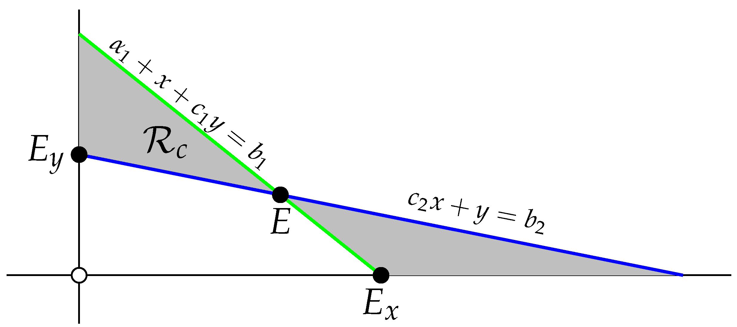
Let ${\alpha }_1\ge b_1$. Lemma 3(c) and (d) guarantee that for initial conditions on the positive y-axis, $\tilde{T}(x_0,y_0)=E_y$ and for initial conditions on the positive x-axis, ${\lim }_{n\to \infty }{\tilde{T}}^n(x_0,y_0)=(0,0)$. To treat the dynamics in the interior of ${\mathbb{R}}_{+}^2$, consider ${\mathcal{R}}_a:=\{(x,y):x,y\ge 0\mathrm{and}{c}_{2}x+y\le b_2\}$. By Theorem 2 of [4], ${\mathcal{R}}_a$ is invariant. The region ${\mathcal{R}}_a$ also attracts the interior of ${\mathbb{R}}_{+}^2$. To verify this, suppose that $(x_0,y_0)\notin {\mathcal{R}}_a$ with $x_0,y_0>0$. In this case $c_2{x}_0+y_0>b_2$ and

$$x_1=\frac{b_1{x}_0}{{\alpha }_1+x_0+c_1{y}_0}<x_0\mathrm{and}{y}_1=\frac{b_2{y}_0}{c_2{x}_0+y_0}<y_0.$$

It follows that there exists $N>0$ such that for all $n\ge N$, $(x_n,y_n)\in {\mathcal{R}}_a$ and thus ${\mathcal{R}}_a$ is attracting. To conclude the proof, suppose $(x_0,y_0)\in {\mathcal{R}}_a$ with $x_0,y_0>0$. In this case $x_1<x_0$, $y_1\ge y_0$ and as a consequence of the invariance of ${\mathcal{R}}_a$, $\left\{x_n\right\}$ is a decreasing sequence while $\left\{y_n\right\}$ is a non-decreasing sequence. Therefore, ${\lim }_{n\to \infty }{\tilde{T}}^n(x_0,y_0)=E_y$. The above arguments prove that the basins of attraction for $E_y$ and the singular point $(0,0)$ are $\mathcal{B}\left(E_y\right)=[0,\infty )\times (0,\infty )$ and $\mathcal{B}(0,0)=[0,\infty )\times \left\{0\right\}$.

(b)

Let ${\alpha }_1<b_1$, $b_1>{\alpha }_1+b_2{c}_1$, and $b_2<c_2(b_1-{\alpha }_1)$. Lemma 3(c) and (d) guarantee that for all initial conditions on the positive y-axis, $\tilde{T}(x_0,y_0)=E_y$ and for all initial conditions on the positive x-axis, ${\lim }_{n\to \infty }{\tilde{T}}^n(x_0,y_0)=E_x$. To treat the interior of ${\mathbb{R}}_{+}^2$, consider ${\mathcal{R}}_b:=\{(x,y):x,y\ge 0,c_{2}x+y\ge b_2\mathrm{and}{\alpha }_1+x+c_{1}y\le b_1\}$ shown in Figure 4.

Please note that ${\mathcal{R}}_b$ is an invariant region by Theorem 2 of [4]. Consider $(x_0,y_0)\in {\mathcal{R}}_b$ with $x_0,y_0>0$ and notice

$$x_1=\frac{b_1{x}_0}{{\alpha }_1+x_0+c_1{y}_0}\ge x_0\mathrm{and}{y}_1=\frac{b_2{y}_0}{c_2{x}_0+y_0}\le y_0.$$

As a consequence of the invariance of ${\mathcal{R}}_b$, $\left\{x_n\right\}$ is a non-decreasing sequence and $\left\{y_n\right\}$ is a non-increasing sequence. Therefore, using basic properties of sequences and the fact that $\tilde{T}$ is strongly competitive, ${\lim }_{n\to \infty }{\tilde{T}}^n(x_0,y_0)=E_x$. Finally, suppose $(x_0,y_0)\notin {\mathcal{R}}_b$ with $x_0,y_0>0$. By Lemma 3(a), $(x_n,y_n)\in [0,b_1)\times [0,b_2]$ for all $n\ge 1$. Choose $(u,v)\in {\mathcal{R}}_b$ with $u,v>0$ such that $(u,v){⪯}_{se}(x_1,y_1){⪯}_{se}(x_1,0)$. Since $\tilde{T}$ is strongly competitive, notice

$${\tilde{T}}^n(u,v){\ll }_{se}{\tilde{T}}^n(x_1,y_1){\ll }_{se}{\tilde{T}}^n(x_1,0).$$

(16)

Therefore, ${\lim }_{n\to \infty }{\tilde{T}}^n(x_0,y_0)=E_x$. We have arrived at the desired result that the basins of attraction for $E_x$ and $E_y$ are $\mathcal{B}\left(E_x\right)=(0,\infty )\times [0,\infty )$ and $\mathcal{B}\left(E_y\right)=\left\{0\right\}\times (0,\infty )$.

The proof for the case when $b_1<{\alpha }_1+b_2{c}_1$, $b_2>c_2(b_1-{\alpha }_1)$ is similar and will be omitted.

(c)

Let ${\alpha }_1<b_1$, $b_1>{\alpha }_1+b_2{c}_1$, and $b_2>c_2(b_1-{\alpha }_1)$. As in part (b), Lemma 3(c) and (d) guarantee that the positive part of the y-axis is a subset of $\mathcal{B}\left(E_y\right)$ and the positive part of the x-axis is a subset of $\mathcal{B}\left(E_x\right)$. To treat the interior of ${\mathbb{R}}_{+}^2$, consider the region ${\mathcal{R}}_c$ shown in Figure 5.

Please note that ${\mathcal{R}}_c$ is invariant by Theorem 2 of [4]. Provided that $(x_0,y_0)\in {\mathcal{R}}_c$ with $x_0,y_0>0$, monotonicity properties (similar to part (a) and (b)) along with Lemma 3(b) can be used to prove that ${\lim }_{n\to \infty }{\tilde{T}}^n(x_0,y_0)=E$. Suppose $(x_0,y_0)\notin {\mathcal{R}}_c$ with $x_0,y_0>0$. By Lemma 3(a) we know that $(x_n,y_n)\in [0,b_1)\times [0,b_2]$ for all $n\ge 1$. Moreover, since $(x_0,y_0){⪯}_{se}(x_0,0)$ then ${\tilde{T}}^n(x_0,y_0){\ll }_{se}{\tilde{T}}^n(x_0,0)$ for all $n\ge 1$. Consequently, there must exist an $N\ge 1$ such that $(x_N,y_N)\in [0,\frac{b_2}{c_2})\times [0,b_2]$. Now, choose $(u,v),(s,t)\in {\mathcal{R}}_c$ such that $(u,v){⪯}_{se}(x_N,y_N){⪯}_{se}(s,t)$. Since $\tilde{T}$ is strongly competitive we have

$${\tilde{T}}^n(u,v){\ll }_{se}{\tilde{T}}^n(x_N,y_N){\ll }_{se}{\tilde{T}}^n(s,t).$$

(17)

Therefore, ${\lim }_{n\to \infty }{\tilde{T}}^n(x_0,y_0)=E$ for all $(x_0,y_0)\notin {\mathcal{R}}_c$. We have reached the desired result that the basins of attraction for $E,E_x$ and $E_y$ are $\mathcal{B}\left(E\right)=(0,\infty )\times (0,\infty )$, $\mathcal{B}\left(E_x\right)=(0,\infty )\times \left\{0\right\}$ and $\mathcal{B}\left(E_y\right)=\left\{0\right\}\times (0,\infty )$.

(d)

Let ${\alpha }_1<b_1$, $b_1<{\alpha }_1+b_2{c}_1$, and $b_2<c_2(b_1-{\alpha }_1)$. In light of Lemma 4(c), Theorems 1 and 5 of [6] guarantees that there exist the global stable and unstable manifolds for E, ${\mathcal{W}}^s\left(E\right)$ and ${\mathcal{W}}^u\left(E\right)$ respectively, with the above mentioned properties. An immediate checking shows that $E_y{⪯}_{se}E{⪯}_{se}{E}_x$ and that the interior of the ordered interval $〚E_y,E〛$ is a subset of $\mathcal{B}\left(E_y\right)$, while the interior of the ordered interval $〚E,E_x〛$ is a subset of $\mathcal{B}\left(E_x\right)$. Now, take any point $(x_0,y_0)\in {\mathbb{R}}_{+}^2$ such that $(x_0,y_0){\prec }_{se}{\mathcal{W}}^s\left(E\right)$ (i.e., above ${\mathcal{W}}^s\left(E\right)$). Then $(0,y_0){⪯}_{se}(x_0,y_0){\prec }_{se}(x_{{\mathcal{W}}^s\left(E\right)},y_0)$, where $(x_{{\mathcal{W}}^s\left(E\right)},y_0)\in {\mathcal{W}}^s\left(E\right)$. By Lemma 3(c) and the monotonicity of $\tilde{T}$, for $n\ge 1$,

$$E_y={\tilde{T}}^n\left((0,y_0)\right){\ll }_{se}{\tilde{T}}^n\left((x_0,y_0)\right){\ll }_{se}{\tilde{T}}^n\left((x_{{\mathcal{W}}^s\left(E\right)},y_0)\right).$$

(18)

Since ${\lim }_{n\to \infty }{\tilde{T}}^n\left((x_{{\mathcal{W}}^s\left(E\right)},y_0)\right)=E$, (18) implies that ${\tilde{T}}^n\left((x_0,y_0)\right)$ enters the ordered interval $〚E_y,E〛$ and so converges to $E_y$. In a similar way, one can show that the ordered interval $〚E,E_x〛$ attracts all points below ${\mathcal{W}}^s\left(E\right)$, and so all such points converge to $E_x$.

(e)

By Theorem 1 of [6], for each $E_t$ there exists the set ${\mathcal{W}}^s\left(E_t\right)$ passing through $E_t$ and asymptotic to $(0,0)$, which is the graph of a continuous, non-decreasing function, which is exactly the basin of attraction of $E_t$. The continuity of the limiting equilibrium solution as a function of initial conditions follows as in [9].

(f)

The proof is similar to the proof of part (b) and will be omitted here.

□

Based on Figure 2 and Figure 3, the global dynamics of systems (4) and (5) are similar. However, the techniques of the proofs are different since the determinant of the map corresponding to system (4) is identically zero in the first quadrant while the determinant of the map corresponding to (5) is positive and the map satisfies $(O+)$ condition. This condition greatly simplifies the proof for system (5). The qualitative difference between system (1) and systems (4) and (5) is in the case when $b_1\le 1,b_2\le 1$ which is possible because of the fact that ${\alpha }_1,{\alpha }_2>0$. In this case, $E_0(0,0)$ is a globally asymptotically stable equilibrium for system (1), while the basin of attraction of the singular point $E_0(0,0)$ is an empty set for system (4), and the basin of attraction of the singular point $E_0(0,0)$ is the non-negative part of the x-axis for system (5). The major difference between systems (4) and (5) is the case ${\alpha }_1\ge b_1$ which is possible only for system (5) when the singular point $(0,0)$ has non-empty basin of attraction. Thus the presence of ${\alpha }_1$ will introduce new dynamic scenario while the presence of both ${\alpha }_1,{\alpha }_2$ will introduce one additional dynamic scenario. As we mentioned in Remark 1 systems (1) and (4) are solvable for the special values of parameters while there is not a formula for the exact solution of system (5) at this time for any choice of parameters.

5. Conclusions

The presented results will serve as motivation for deriving the general results for monotone (competitive and cooperative) systems in the plane such as in [24], which will lead to some standard global dynamic scenarios results. The global dynamic scenarios results require detailed local stability analysis which can be fairly complicated and tedious as soon as at least one quadratic term is present, see for instance [25]. The presence of quadratic terms may cause the emergence of new dynamic scenarios such as the Allee effect, periodic solutions, Naimark-Sacker bifurcation etc. Furthermore, we are interested in extending the presented results to higher dimensions to so called multispecies Leslie-Gower model which will consist of $k\ge 3$ equation of type (1). Some results in this direction were obtained in [11,12]. We would like to use the full strength of monotone systems theory which at this moment is not available in dimensions higher than 2. The $k\ge 3$ dimensional version of System (4) will be an example of linear fractional homogeneous system which dynamics can be reduced to dynamics of $k-1$ linear fractional homogeneous system, which means that the dynamics 3-dimensional version of System (4) can be reduced to dynamics of this system. In some special cases analogue to the ones in Remark 1 one can find the explicit solution of such system and so obtain the dynamics in such case.

References

- Cushing, J.M.; Levarge, S.; Chitnis, N.; Henson, S.M. Some discrete competition models and the competitive exclusion principle. J. Differ. Equ. Appl. 2004, 10, 1139–1152. [Google Scholar] [CrossRef]
- Cushing, J.M.; Levarge, S. Some discrete competition models and the principle of competitive exclusion. In Difference Equations and Discrete Dynamical Systems; World Scientific: Hackensack, NJ, USA, 2005; pp. 283–301. [Google Scholar]
- Cushing, J.M.; Henson, S.M.; Blackburn, C.C. Multiple mixed-type attractors in a competition model. J. Biol. Dyn. 2007, 1, 347–362. [Google Scholar] [CrossRef] [PubMed] [Green Version]
- Kulenović, M.R.S.; Merino, O. Competitive-Exclusion versus Competitive-Coexistence for Systems in the Plane. Discret. Contin. Dyn. Syst. Ser. B 2006, 6, 1141–1156. [Google Scholar]
- Kulenović, M.R.S.; Merino, O. Global Bifurcation for Competitive Systems in the Plane. Discret. Contin. Dyn. Syst. B 2009, 12, 133–149. [Google Scholar]
- Kulenović, M.R.S.; Merino, O. Invariant Manifolds for Competitive Discrete Systems in the Plane. Int. J. Bifurc. Chaos 2010, 20, 2471–2486. [Google Scholar] [CrossRef]
- Smith, H.L. Planar Competitive and Cooperative Difference Equations. J. Differ. Equ. Appl. 1998, 3, 335–357. [Google Scholar] [CrossRef]
- Camouzis, E.; Kulenović, M.R.S.; Ladas, G.; Merino, O. Rational Systems in the Plane-Open Problems and Conjectures. J. Differ. Equ. Appl. 2009, 15, 303–323. [Google Scholar] [CrossRef]
- Burgić, D.; Kalabušić, S.; Kulenović, M.R.S. Non-hyperbolic Dynamics for Competitive Systems in the Plane and Global Period-doubling Bifurcations. Adv. Dyn. Syst. Appl. 2008, 3, 229–249. [Google Scholar]
- Sacker, R. Global stability in a multi-species periodic Leslie-Gower model. J. Biol. Dyn. 2011, 5, 549–562. [Google Scholar] [CrossRef]
- Sacker, R. An invariance theorem for mappings. J. Differ. Equ. Appl. 2012, 18, 163–166. [Google Scholar] [CrossRef]
- Sacker, R. A note: An invariance theorem for mappings II. J. Dyn. Differ. Equ. 2012, 24, 595–599. [Google Scholar] [CrossRef]
- Kulenović, M.R.S.; Ladas, G. Dynamics of Second Order Rational Difference Equations with Open Problems and Conjectures; Chapman and Hall/CRC: Boca Raton, FL, USA; London, UK, 2001. [Google Scholar]
- Clark, D.; Kulenović, M.R.S.; Selgrade, J.F. Global Asymptotic Behavior of a Two Dimensional Difference Equation Modelling Competition. Nonlinear Anal. TMA 2003, 52, 1765–1776. [Google Scholar] [CrossRef]
- Hess, P. Periodic-Parabolic Boundary Value Problems and Positivity; Pitman Research Notes in Mathematics Series, 247; Longman Scientific & Technical: Harlow, UK, 1991; pp. 619–620. [Google Scholar]
- Kalabušić, S.; Kulenović, M.R.S.; Pilav, E. Dynamics of a two-dimensional system of rational difference equations of Leslie-Gower type. Adv. Differ. Equ. 2011, 229, 29. [Google Scholar] [CrossRef]
- Kulenović, M.R.S.; Nurkanović, M. Asymptotic Behavior of a Linear Fractional System of Difference Equations. J. Inequal. Appl. 2005, 2005, 127–143. [Google Scholar] [CrossRef]
- Leonard, W.J.; May, R. Nonlinear aspects of competition between species. SIAM J. Appl. Math. 1975, 29, 243–275. [Google Scholar]
- Smale, S. On the differential equations of species in competition. J. Math. Biol. 1976, 3, 5–7. [Google Scholar] [CrossRef] [PubMed]
- de Mottoni, P.; Schiaffino, A. Competition systems with periodic coefficients: A geometric approach. J. Math. Biol. 1981, 11, 319–335. [Google Scholar] [CrossRef]
- Smith, H.L. Periodic competitive differential equations and the discrete dynamics of competitive maps. J. Differ. Equ. 1986, 64, 165–194. [Google Scholar] [CrossRef] [Green Version]
- Huang, Y.S.; Knopf, P.M. Global convergence properties of first-order homogeneous systems of rational difference equations. J. Differ. Equ. Appl. 2012, 18, 1683–1707. [Google Scholar] [CrossRef]
- Hirsch, M.; Smith, H. Monotone dynamical systems. In Handbook of Differential Equations: Ordinary Differential Equations; Elsevier B. V.: Amsterdam, The Netherlands, 2005; Volume II, pp. 239–357. [Google Scholar]
- Bertrand, E.; Kulenović, M.R.S. Global Dynamic Scenarios for Competitive Maps in the Plane. Adv. Differ. Equ. 2018. [Google Scholar] [CrossRef]
- Brett, A.; Kulenović, M.R.S. Two Species Competitive Model with the Allee Effect. Adv. Differ. Equ. 2014, 2014, 307. [Google Scholar] [CrossRef]