Weighted Block Golub-Kahan-Lanczos Algorithms for Linear Response Eigenvalue Problem


1
School of Science, Jiangnan University, Wuxi 214122, China
2
College of Computer and Information Science, Fujian Agriculture and Forestry University, Fuzhou 350002, China
3
School of Mathematical Sciences, Shanghai Key Laboratory of PMMP, East China Normal University, Shanghai 200241, China
*
Author to whom correspondence should be addressed.
Mathematics 2019, 7(1), 53; https://doi.org/10.3390/math7010053
Submission received: 30 November 2018
/
Revised: 25 December 2018
/
Accepted: 29 December 2018
/
Published: 7 January 2019
(This article belongs to the Special Issue Mathematics and Engineering)
Abstract
:In order to solve all or some eigenvalues lied in a cluster, we propose a weighted block Golub-Kahan-Lanczos algorithm for the linear response eigenvalue problem. Error bounds of the approximations to an eigenvalue cluster, as well as their corresponding eigenspace, are established and show the advantages. A practical thick-restart strategy is applied to the block algorithm to eliminate the increasing computational and memory costs, and the numerical instability. Numerical examples illustrate the effectiveness of our new algorithms.
Keywords:
linear response eigenvalue problem; block methods; weighted Golub-Kahan-Lanczos algorithm; convergence analysis; thick restartAMS Subject Classification:
65F15; 15A181. Introduction
In this paper, we are interested in solving the linear response eigenvalue problem (LREP):
where K and M are real symmetric positive definite matrices. Such a problem arises from studying the excitation energy of many particle systems in computational quantum chemistry and physics [1,2,3]. It also known as the Bethe-Salpeter (BS) eigenvalue-problem [4] or the random phase approximation (RPA) eigenvalue problem [5]. There has immense past and recent work in developing efficient numerical algorithms and attractive theories for LREP [6,7,8,9,10,11,12,13,14,15].
Since all the eigenvalues of are real nonzero and appear in pairs [6], thus we order the eigenvalues in ascending order, i.e.,
In this paper, we focus on a small portion of the positive eigenvalues for LREP, i.e., , with and , and their corresponding eigenvectors. We only consider the real case, all the results can be easily applied to the complex case.
The weighted Golub-Kahan-Lanczos method (wGKL) for LREP was introduced in [16]. It produces recursively a much small projection of at j-th iteration, where is upper bidiagonal. Afterwards, the eigenpairs of can be constructed by the singular value decomposition of . The convergence analysis performs that running k iterations of wGKL is equivalently running iterations of a weighted Lanczos algorithm for [16]. Actually, can be also a lower bidiagonal matrix, and the same discussion can be taken place as in the case of is upper bidiagonal. In the following, we only consider the upper bidiagonal case.
It is well known that the single-vector Lanczos method is widely used for searching a small number of extreme eigenvalues, and it may encounter very slow convergence when the wanted eigenvalues stay in a cluster [17]. Instead, a block Lanczos method with a suitable block size is capable of computing a cluster of eigenvalues including multiple eigenvalues very quickly. Motivated by this idea, we are going to develop a block version of wGKL in [16] in order to find efficiently all or some positive eigenvalues within a cluster for LREP. Based on the standard block Lanczos convergence theory in [17], the error bounds of approximation to an eigenvalue cluster, as well as their corresponding eigenspace are established to illustrate the advantage of our weighted block Golub-Kahan-Lanczos algorithm (wbGKL).
As the increasing size of the Krylov subspace, the storage demands, computational costs, and numerical stability of a simple version of a block Lanczos method may be affected [18]. Several kinds of efficiently restarting strategies to eliminate these effects are developed for the classic Lanczos method, such as, implicitly restart method [19], thick restart method [20]. In order to make our block method more practical, and using the special structure of LREP, we consider the thick restart strategy to our block method.
The rest of this paper is organized as follows. Section 2 gives some necessary preliminaries for our later use. In Section 3, the weighted block Golub-Kahan-Lanczos algorithm (wbGKL) for LREP is presented, and its convergence analysis is discussed. Section 4 proposed the thick restart weighted block Golub-Kahan-Lanczos algorithm (wbGKL-TR). The numerical examples are tested in Section 5 to illustrate the efficiency of our new algorithms. Finally, some conclusions are given in Section 6.
Throughout this paper, is the set of all real matrices, , and . (or simply I if its dimension is clear from the context) is the identity matrix, and is an matrix of zero. The superscript “” denotes transpose. denotes the Frobenius norm of a matrix, and denotes the 2-norm of a matrix or a vector. For a matrix , denotes the rank of X, and denotes the column space of X; the submatrices and of X composed by the intersections of row i to row j and column k to column ℓ, respectively. For matrices or scalars , denotes the block diagonal matrix with the i-th diagonal block .
2. Preliminaries
For a symmetric positive definite matrix , the W-inner product is defined as following
If , then we denote it by , and call it with x and y are W-orthogonal. The projector is called the W-orthogonal projector onto if for any ,
For two subspaces , and suppose , if and are W-orthonormal basis of and , respectively, i.e.,
and for with are the singular values of , then the W-canonical angles from to are defined by
If , these angles can be said between and . Obviously, . Set
Especially, if , X is a vector, there is only one W-canonical angle from to . In the following, we may use a matrix in one or both arguments of , i.e., with the understanding that it means the subspace spanned by the columns of the matrix argument.
The following two lemmas are important to our later analysis, and for proofs and more details, the reader is referred to [12,16].
Lemma 1.
([12] Lemma 3.2). Let and be two subspaces in with equal dimensional . Suppose . Then, for any set of the basis vectors in where , there is a set of linearly independent vectors in such that for , where is the W-orthogonal projector onto .
Lemma 2.
([16] Proposition 3.1). The matrix has N position eigenvalues with . The corresponding right eigenvectors can be chosen K-orthonormal, and the corresponding left eigenvectors can be chosen M-orthonormal. In particular, for given , one can choose , and for given , , for .
3. Weighted Block Golub-Kahan-Lanczos Algorithm
3.1. Weighted Block Golub-Kahan-Lanczos Algorithm
In this section, we plan to introduce the weighted block Golub-Kahan-Lanczos algorithm (wbGKL) for LREP, which is a block version of the weighted Golub-Kahan-Lanczos algorithm [16]. Algorithm 1 gives the process of recursively generating the M-orthonormal matrix , the K-orthonormal matrix , and the block bidiagonal matrix . Giving with , denoting , and
then we have the relation from Algorithm 1:
and
Remark 1.
In Algorithm 1, we only consider the case that , no further treatment is provided for the cases or . Because K and M are both symmetric positive definite, thus the two W inStep 2are both reversible.
| Algorithm 1: wbGKL |
| 1. Choose satisfying , and set , , . Compute . 2. For Do Cholesky decomposition , , % means Do Cholesky decomposition , , End |
Remark 2.
With j increasing inStep 2, the M-orthogonality of and the K-orthogonality of will slowly lose. Thus, in practice, we can add a re-orthogonalization process in each iteration to eliminate the defect. The same strategy is executed in the following algorithms.
From (1), we have
with . Then, the approximate eigenpairs of can be obtained by solving a small eigenvalue problem of . Suppose has an singular value decomposition
where , , with . Thus, we can take as the Ritz values of and
as the corresponding -orthonormal Ritz vectors, where .
3.2. Convergence Analysis
In this section, we first consider the convergence analysis when using the first few as approximations to the first few . Then, the similar theories are presented if using the last few as approximations to the last few . Since a block Lanczos method with a suitable block size which is not smaller than the size of an eigenvalue cluster can compute all eigenvalues in the cluster. Now, we are considering the i-th to -st eigenpairs of LREP, in which the k-th to ℓ-th eigenvalues form a cluster as in the following figure with and .

Here, the squares of the eigenvalues for LREP are listed. Hence, motivated by [12,17], we analyze the convergence of the cluster eigenvalues and their corresponding eigenspace, and give the error bounds of the approximate eigenpairs belonging to eigenvalue cluster together, instead of separately for each individual eigenpair.
We first give some notations and equations, which are critical in our main theorem. Note that from (1), we get
Since (2) is the singular value decomposition of , thus the eigenvalues of are with the associated eigenvectors for .
From Lemma 2, if we let , and , then , and
Write and as
![Mathematics 07 00053 i003]()

Let and . Denote the first kind Chebyshev polynomial with j-th degree, and .
In the following, we assume
i.e., , then from Lemma 1, we have ∃ with , s.t.,
Theorem 1.
Suppose , and Z satisfy (6), then we have
with
and
with constant c lies between 1 and , and if , and
Particularly if , then
Proof.
Multiplying from left, (4) can be rewritten as , so, is the eigenpair of , for , and are orthonormal. Do the same process to (3), we have
where , , and , which can be seen as the relation generalize by using standard Lanczos process to . Thus, are the Ritz values of , with the corresponding orthonormal Ritz vectors .
Premultiplying to Equation (6), we have . Consequently, the conditions of the block Lanczos convergence Theorem 4.1 and Theorem 5.1 in [17] are satisfied. Thus, using the results Theorem 5.1 in [17], one has
Let , then is the orthogonal projection onto , thus from (9), we have
Consequently, applying the results of Theorem 4.1 in [17], we get
Theorem 1 is used to bound the errors of the approximate eigenvalues to an eigenvalue cluster including the multiple eigenvalues. It can be also applied to the single eigenvalue case, the following corollary is derived by setting , except the left equality of (10), which needs to be proved.
Corollary 1.
Suppose , then for , there exits a vector , s.t., , and
with
and
with
Proof.
We only proof the left equality of (11). From (4) and Lemma 2, we have . If we let , and , then we can get by using . Thus
Then,
☐
Next, we are going to consider the last few to approximate as the last few , , and to form a cluster in to , which is described in the following figure, where , , , and .

Similar to the above discussion for the first few eigenvalues, we can also obtain the error bounds of the approximate last few eigenpairs belongs to eigenvalue cluster together. We use the same notion, except and . Assuming , then from Lemma 1, there ∃ with , s.t.,
Theorem 2.
Remark 3.
Similar to Corollary 1, Theorem 2 can also be applied to the single eigenvalue case, here we omit the detail.
Remark 4.
In Theorem 1 and 2, we use the Frobenius norm to estimate the accuracy of eigenpairs approximations, in fact, any unitary invariant norm can be used to measure.
Remark 5.
Compared with the single-vector type of the weighted Golub-Kahan-Lanczos method in [16], our convergence results show the superiority of the block version. For instance, in Corollary 1, the convergence rate of the approximate eigenvalues is proportional to with , which is obviously better than with in ([16] Theorem 3.4). While the additional cost caused from the block version can be paid by the improvements generated by , especially when the desired eigenvalues lie in a well-separated cluster [12].
4. Thick Restart
As the number of iterations increases, Algorithm 1 may encounter the dilemma that the amount of calculation and storage increases sharply and the numerical stability gradually weakens. In this section, we will apply the thick restart strategy [20] to improve the algorithm. After running n iterations, Algorithm 1 derives the following relations for LREP:
with .
Recall the SVD (2), let and be the first columns of and , respectively, i.e.,
Thus it follows that
where .
By using the approximate eigenvectors of for thick restart, we post-multiply and to the Equation (15), respectively, and get
Next, and will be generalized. Firstly, we compute
From the second equation in (18), we know . Do Cholesky decomposition , and set , . Compute , and let
we have
Secondly, from the above equation, we can compute
Again using (19), it is easily got that . Similarly, do Cholesky decomposition , and let , . Compute , and let , we get
Continue the same procedure for and , we can obtain the new M-orthonormal matrix , the new K-orthonormal matrix , and the new matrix , and relations
with , and
Note that is no longer a block bidiagonal matrix. Algorithm 2 is our thick-restart weighted block Golub-Kahan-Lanczos algorithm for LREP.
Remark 6.
Actually, from the construction of , we can know the procedure for getting and is the same as applying Algorithm 1 to for iterations, thus we use Algorithm 1 directly in restartingStep 2of the following Algorithm 2.
| Algorithm 2: wbGKL-TR |
| 1. Given an initial guess satisfying , a tolerance , an integer k that the k blocks approximate eigenvectors we want to add to the solving subspace, an integer n the block dimension of solving subspace, as well as the desired number of eigenpairs; 2. Apply Algorithm 1 from the current point to generate the rest of , , and . If it is the first cycle, the current point is , else ; 3. Compute an SVD of as in (2), select wanted singular values , and their associated left singular vectors and right singular vectors . Form the approximate eigenpairs for , if the stopping criterion is satisfied, then stop, else continue; 4. Generate new , and : Compute , , , , , ; Compute , do Cholesky decomposition , set , , ; Compute , do Cholesky decomposition , set , , ; Let , , , and go to Step 2. |
Remark 7.
InStep 3, we compute the harmonic Ritz pairs after n iterations. In practice, we do the computation for each iterations . When restarting, the information chosen to add to the solving subspaces are the wanted singular values of with their corresponding left and right singular vectors. Actually, we use MATLAB command “sort” to choose the smallest ones or the largest ones, and which singular values to choose depends on the desired eigenvalues of .
In the end of this section, we list the computational costs in a generic cycle of four algorithms, which are weighted block Golub-Kahan-Lanczos algorithm, thick-restart weighted block Golub-Kahan-Lanczos algorithm, block Lanczos algorithm [12], and thick-restart block Lanczos algorithm [12], and denoted by wbGKL, wbGKL-TR, BLan, and BLan-TR, respectively. The detail pseudocodes of BLan and BLan-TR are be found in [12].
The comparisons are presented in Table 1 and Table 2. Here, we denote “block vector” a rectangular matrix, denote “mvb” the product number of a matrix and a block vector. “dpb” denotes the dot product number of two block vectors X and Y, i.e., . “saxpyb” denotes the number of adding two block vectors or multiplying a block vector to a small matrix. “Ep()(with sorting)” means the number of size eigenvalue problem with sorting eigenvalues and their corresponding eigenvectors in one cycle. Similarly, “Sp()” denotes the number of size singular value decomposition in one cycle. Because wbGKL and BLan are non-restart algorithms, we just count the first n Lanczos iterations.
5. Numerical Examples
In this section, two numerical experiments are carried out by using MATLAB 8.4 (R2014b) on a laptop with an Intel Core i5-6200U CPU 2.3 GHz memory 8 GB under the Windows 10 operating system.
Example 1.
In this example, we check the bounds established in Theorem 1 and 2. For simplicity, we take , the number of weighted block Golub-Kahan-Lanczos steps , as diagonal matrix , where
and , , , , . There are three positive eigenvalue clusters: , , or . Obviously, .
We seek two groups of the approximate eigenpairs, the first is related to the first cluster, the second is related to the last cluster, i.e., approximate , and approximate . In order to see the affect that generated from to the upper bounds of the approximate eigenpairs errors in weighted block Golub-Kahan-Lanczos method for LREP, we change the parameter to overmaster the tightness among eigenvalues within and . First, we choose the same matrix as in [12,17], i.e.,
Obviously, and . Since K symmetric positive definite, thus do Cholesky decomposition , let , hence, satisfies (5), i.e., is singular. We take , then Z satisfies (6). We execute the weighted block Golub-Kahan-Lanczos method with full re-orthogonalization for LREP in MATLAB, and check the bounds in (7), (8), (13), and (14). Since the approximate eigenvalues are and , thus , , and we measure the following two groups of errors:
and
Actually, and are upper bounds of and , and and are upper bounds of and . Table 3 and Table 4 report the results of , , with the parameter goes to 0. From the two tables, we can see that the bounds for the eigenvalues lie in a cluster and their corresponding eigenvectors are sharp, and they are not sensitive to when goes to 0.
Example 2.
In this example, we are going to test the effectiveness of our weighted block Golub-Kahan-Lanczos algorithms. Four algorithms are tested, i.e.,wbGKL,wbGKL-TR,BLan, andBLan-TR. We choose 3 test problems used in [12,13], which are listed in Table 5. All the matrices K and M in the problems are symmetric positive definite. Specifically, Test 1 and Test 2, which are derived by the turboTDDFT command in QUANTUM ESPRESSO [22], are from the linear response research for Na2 and silane (SiH4) compound, respectively. The matrices K and M in Test 3 are from the University of Florida Sparse Matrix Collection [23], where the order of K is , and M is the leading principal submatrix of .
We aim to compute the smallest 5 positive eigenvalues and the largest 5 eigenvalues, i.e., for , together with their associated eigenvectors. The initial guess is chosen as with block size , where is the MATLAB command. The same as in Example 1, since K is symmetric positive definite, thus do Cholesky decomposition , let , hence, satisfies . In wbGKL-TR and BLan-TR, we select , , i.e., the restart will occur once the dimension of the solving subspace is larger than 90, and the information of 60 Ritz vectors are kept. For wbGKL and BLan, because there is no restart, then we compute the approximate eigenpairs when the Lanczos iterations equals to , , hence, the Lanczos iterations are as the same amount as in wbGKL-TR and BLan-TR. The following relative eigenvalue error and relative residual 1-norm for each 10 approximate eigenpairs are calculated:
where the “exact” eigenvalues are calculated by the MATLAB code . The calculated approximate eigenpair is regarded as converged if .
Table 6 and Table 7 give the number of the Lanczos iterations (denote by ) and the CPU time in seconds (denote by ) for the four algorithms, and Table 6 is for the smallest 5 positive eigenvalues, Table 7 is for the largest 5 eigenvalues. From Table 6, one can see that, no matter the smallest or the largest eigenvalues, the iteration number of the four algorithms are competitive, but wbGKL and wbGKL-TR cost significant less time than BLan and BLan-TR, especially, wbGKL-TR consumes the least amount of time. Because BLan and BLan-TR need to compute the eigenvalues of , which is a nonsymmetric matrix, thus the two algorithms slower than wbGKL and wbGKL-TR. Due to the saving during the orthogonalization procedure and solving a much smaller , wbGKL-TR is the faster algorithm.
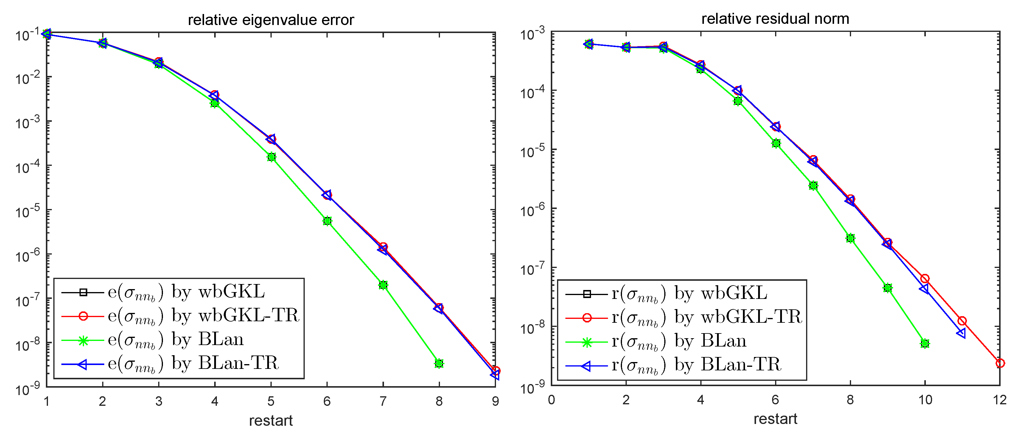
The accuracy of the last two approximate eigenpairs in Test 1 are shown in Figure 1. From the figure, we can see that, for the last two eigenpairs, wbGKL and BLan require almost the same iterations to obtain the same accuracy, and the case of wbGKL-TR and BLan-TR also need almost the same iterations, which are one or two more restarts than wbGKL and BLan. On one hand, without solving a nonsymmetric eigenproblem, wbGKL and wbGKL-TR can save much more time than BLan and BLan-TR. On the other hand, since the dimension of the solving subspace for wbGKL-TR is bounded by , the savings in the process of orthogonalization and a much smaller singular value decomposition problem is sufficient to cover the additional restart steps.
6. Conclusions
In this paper, we present a weighted block Golub-Kahan-Lanczos algorithm to solve the desired small portion of smallest or largest positive eigenvalues which are in a cluster. Convergence analysis is established in Theorems 1 and 2, and bound the errors of the eigenvalue and eigenvector approximations belonging to an eigenvalue cluster. These results also show the advantages of the block algorithm over the single-vector version. To make the new algorithm more practical, we introduced a thick-restart strategy to eliminate the numerical difficulties caused by the block method. Numerical examples are executed to demonstrate the efficiency of our new restart algorithm.
Author Contributions
Conceptualization, G.C.; Data curation, H.Z. and Z.T.; Formal analysis, H.Z. and Z.T.; Methodology, H.Z.; Project administration, H.Z. and G.C.; Resources, H.Z.; Visualization, H.Z. and Z.T.; Writing—original draft, H.Z.; Writing—review and editing, Z.T. and G.C.
Funding
This work was financial supported by the National Nature Science Foundation of China (No. 11701225, 11601081, 11471122), Fundamental Research Funds for the Central Universities (No. JUSRP11719), Natural Science Foundation of Jiangsu Province (No. BK20170173), and the research fund for distinguished young scholars of Fujian Agriculture and Forestry University (No. xjq201727).
Conflicts of Interest
The authors declare no conflict of interest.
References
- Casida, M.E. Time-Dependent Density Functional Response Theory for Molecules. In Recent Advances in Density Functional Methods; Chong, D.P., Ed.; World Scientific: Singapore, 1995. [Google Scholar]
- Onida, G.; Reining, L.; Rubio, A. Electronic excitations density functional versus many-body Green’s function. Rev. Mod. Phys. 2002, 74, 601–659. [Google Scholar] [CrossRef]
- Rocca, D. Time-Dependent Density Functional Perturbation Theory: New algorithms with Applications to Molecular Spectra. Ph.D. Thesis, The International School for Advanced Studies, Trieste, Italy, 2007. [Google Scholar]
- Shao, M.; da Jornada, F.H.; Yang, C.; Deslippe, J.; Louie, S.G. Structure preserving parallel algorithms for solving the Bethe-Salpeter eigenvalue problem. Linear Algebra Appl. 2016, 488, 148–167. [Google Scholar] [CrossRef]
- Ring, P.; Ma, Z.; Giai, V.N.; Vretenar, D.; Wandelt, A.; Gao, L. The time-dependent relativistic mean-field theory and the random phase approximation. Nucl. Phys. A 2001, 694, 249–268. [Google Scholar] [CrossRef] [Green Version]
- Bai, Z.; Li, R.-C. Minimization principles for the linear response eigenvalue problem I: Theory. SIAM J. Matrix Anal. Appl. 2012, 33, 1075–1100. [Google Scholar] [CrossRef]
- Bai, Z.; Li, R.-C. Minimization principles for the linear response eigenvalue problem II: Computation. SIAM J. Matrix Anal. Appl. 2013, 34, 392–416. [Google Scholar] [CrossRef]
- Bai, Z.; Li, R.-C. Minimization principles and computation for the generalized linear response eigenvalue problem. BIT Numer. Math. 2014, 54, 31–54. [Google Scholar] [CrossRef]
- Li, T.; Li, R.-C.; Lin, W.-W. A symmetric structure-preserving ΓQR algorithm for linear response eigenvalue problems. Linear Algebra Appl. 2017, 520, 191–214. [Google Scholar] [CrossRef]
- Teng, Z.; Li, R.-C. Convergence analysis of Lanczos-type methods for the linear response eigenvalue problem. J. Comput. Appl. Math. 2013, 247, 17–33. [Google Scholar] [CrossRef]
- Teng, Z.; Lu, L.; Li, R.-C. Perturbation of partitioned linear response eigenvalue problems. Electron. Trans. Numer. Anal. 2015, 44, 624–638. [Google Scholar]
- Teng, Z.; Zhang, L.-H. A block Lanczos method for then linear response eigenvalue problem. Electron. Trans. Numer. Anal. 2017, 46, 505–523. [Google Scholar]
- Teng, Z.; Zhou, Y.; Li, R.-C. A block Chebyshev-Davidson method for linear response eigenvalue problems. Adv. Comput. Math. 2016, 42, 1103–1128. [Google Scholar] [CrossRef]
- Zhang, L.-H.; Lin, W.-W.; Li, R.-C. Backward perturbation analysis and residual-based error bounds for the linear response eigenvalue problem. BIT Numer. Math. 2014, 55, 869–896. [Google Scholar] [CrossRef]
- Zhang, L.-H.; Xue, J.; Li, R.-C. Rayleigh-Ritz approximation for the linear response eigenvalue problem. SIAM J. Matrix Anal. Appl. 2014, 35, 765–782. [Google Scholar] [CrossRef]
- Zhong, H.; Xu, H. Weighted Golub-Kahan-Lanczos bidiagonalizaiton algorithms. Electron. Trans. Numer. Anal. 2017, 47, 153–178. [Google Scholar]
- Li, R.-C.; Zhang, L.-H. Convergence of the block Lanczos method for eigenvalue clusters. Numer. Math. 2015, 131, 83–113. [Google Scholar] [CrossRef]
- Chapman, A.; Saad, Y. Deflated and augmented Krylov subspace techniques. Numer. Linear Algebra Appl. 1996, 4, 43–66. [Google Scholar] [CrossRef]
- Lehoucq, R.B.; Sorensen, D.C. Deflation techniques for an implicitly restarted Arnoldi iteration. SIAM J. Matrix Anal. Appl. 1996, 17, 789–821. [Google Scholar] [CrossRef]
- Wu, K.; Simon, H. Thick-restart Lanczos method for large symmetric eigenvalue problems. SIAM J. Matrix Anal. Appl. 2000, 22, 602–616. [Google Scholar] [CrossRef]
- Knyazev, A.V.; Argentati, M.E. Principal angles between subspaces in an A-based scalar product: Algorithms and perturbation estimates. SIAM J. Sci. Comput. 2002, 23, 2008–2040. [Google Scholar] [CrossRef]
- Giannozzi, P.; Baroni, S.; Bonini, N.; Calandra, M.; Car, R.; Cavazzoni, C.; Ceresoli, D.; Chiarotti, G.L.; Cococcioni, M.; Dabo, I.; et al. QUANTUM ESPRESSO: A modular and open-source software project for quantum simulations of materials. J. Phys. Condens. Matter 2009, 21, 395502. [Google Scholar] [CrossRef]
- Davis, T.; Hu, Y. The University of Florida Sparse Matrix Collection. ACM Trans. Math. Softw. 2011, 38, 1:1–1:25. [Google Scholar] [CrossRef]
Figure 1.
Errors and residuals of the 2 smallest positive eigenvalues for Test 1 in Example 2.


Table 1.
Main computational costs per cycle wbGKL and wbGKL-TR.
| wbGKL | wbGKL-TR | wbGKL-TR | |
|---|---|---|---|
| (1-st Cycle) | (Other Cycle) | ||
| mvb | |||
| dpb | |||
| saxpyb | |||
| block vector updates | |||
| Ep()(with sorting) | 0 | 0 | 0 |
| Sp() | 1 | 1 | 1 |
Table 2.
Main computational costs per cycle BLan and BLan-TR.
| BLan | BLan-TR | BLan-TR | |
|---|---|---|---|
| (1-st Cycle) | (Other Cycle) | ||
| mvb | |||
| dpb | |||
| saxpyb | |||
| block vector updates | |||
| Ep()(with sorting) | 1 | 1 | 1 |
| Sp() | 0 | 0 | 0 |
Table 3.
, together with their upper bounds , of Example 1.
Table 4.
, together with their upper bounds , of Example 1.
Table 5.
The matrices K and M in Test 1–3.
| Problems | N | K | M |
|---|---|---|---|
| Test 1 | 1862 | ||
| Test 2 | 5660 | ||
| Test 3 | 9604 |
Table 6.
Compute 5 smallest positive eigenvalues for Test 1–3.
| Algorithms | Test 1 | Test 2 | Test 3 | |||
|---|---|---|---|---|---|---|
| wbGKL | 1.5070 | 149 | 25.7848 | 319 | 15.9308 | 379 |
| wbGKL-TR | 1.0746 | 179 | 20.3593 | 359 | 5.1302 | 589 |
| BLan | 4.6739 | 149 | 87.1670 | 349 | 43.9506 | 379 |
| BLan-TR | 2.1243 | 163 | 39.1306 | 393 | 19.9677 | 592 |
Table 7.
Compute 5 largest eigenvalues for Test 1–3.
| Algorithms | Test 1 | Test 2 | Test 3 | |||
|---|---|---|---|---|---|---|
| wbGKL | 0.6387 | 79 | 12.4658 | 179 | 1.0639 | 109 |
| wbGKL-TR | 0.5284 | 79 | 9.9093 | 179 | 0.8774 | 109 |
| BLan | 1.4634 | 79 | 27.4028 | 179 | 6.7574 | 109 |
| BLan-TR | 1.0151 | 82 | 18.3415 | 186 | 4.1298 | 113 |
© 2019 by the authors. Licensee MDPI, Basel, Switzerland. This article is an open access article distributed under the terms and conditions of the Creative Commons Attribution (CC BY) license (http://creativecommons.org/licenses/by/4.0/).
Share and Cite
MDPI and ACS Style
Zhong, H.; Teng, Z.; Chen, G. Weighted Block Golub-Kahan-Lanczos Algorithms for Linear Response Eigenvalue Problem. Mathematics 2019, 7, 53. https://doi.org/10.3390/math7010053
AMA Style
Zhong H, Teng Z, Chen G. Weighted Block Golub-Kahan-Lanczos Algorithms for Linear Response Eigenvalue Problem. Mathematics. 2019; 7(1):53. https://doi.org/10.3390/math7010053
Chicago/Turabian StyleZhong, Hongxiu, Zhongming Teng, and Guoliang Chen. 2019. "Weighted Block Golub-Kahan-Lanczos Algorithms for Linear Response Eigenvalue Problem" Mathematics 7, no. 1: 53. https://doi.org/10.3390/math7010053
Note that from the first issue of 2016, this journal uses article numbers instead of page numbers. See further details here.