Complex Intuitionistic Fuzzy Graphs with Application in Cellular Network Provider Companies

Abstract

In recent years, a mathematical approach of blending different aspects is on the way, which as a result gives a more generalized approach. Following the above mathematical approach, we combine two very powerful techniques, namely complex intuitionistic fuzzy sets and graph theory, and introduce the notion of complex intuitionistic fuzzy graphs. Then, we introduce certain notions including union, join and composition of complex intuitionistic fuzzy graphs, through which one can easily manipulate the complex intuitionistic fuzzy graphs in decision making problems. We elucidate these operations with some examples. We also describe the homomorphisms of complex intuitionistic fuzzy graphs. Finally, we provide an application in cellular network provider companies for the testing of our approach.

1. Introduction

We divide the Introduction Section into four main paragraphs. In the first paragraph, we provide some details about the fuzzy sets. In the second paragraph, detail is given about the complex version of fuzzy sets, namely complex fuzzy sets, which is an extension of fuzzy sets. In the third paragraph, detail is given about graph theory in terms of different types of fuzzy sets. In the fourth paragraph, we give our presented approach by combining the two different approaches given in the second and third paragraphs.

Fuzzy set theory was conferred by Zadeh [1] to solve difficulties in dealing with uncertainties. Since then, the theory of fuzzy sets and fuzzy logic have been examined by many researchers to solve many real life problems involving ambiguous and uncertain environment. Atanassov [2] proposed the extended form of fuzzy set by adding a new component, called “intuitionistic fuzzy sets” ($IF$-sets). The idea of $IF$-sets is more meaningful as well as intensive due to the presence of degree of truth and falsity membership. Applications of these sets have been broadly studied in other aspects such as image processing [3], multi-criteria decision making [4], pattern recognition [5], etc.

Buckley [6] and Nguyen et al. [7] combined complex numbers with fuzzy sets. On the other hand, Ramot et al. [8,9] extended the range of membership to “unit circle in the complex plane”, unlike others who limited the range to $[0,1]$. Zhang et al. [10] studied some operation properties and $\delta$-equalities of complex fuzzy sets. Some applications of complex fuzzy sets have been considered in reasoning schemes [11], image restoration [12] and decision making [13]. Further, this concept has been studied in intuitionistic fuzzy sets [14]. Alkouri and Salleh studied some operations on complex Atanassov’s intuitionistic fuzzy sets in [15] and also studied complex Atanassov’s intuitionistic fuzzy relation in [16]. Ali et al. [17] introduced complex intuitionistic fuzzy classes.

Fuzzy graphs were narrated by Rosenfeld [18] and Mordeson [19]. After that, some opinion on “fuzzy graphs” were given by Bhattacharya [20]. He showed that none of the concepts of crisp graph theory have similarities in fuzzy graphs. Thirunavukarasu et al. [21] extended this concept for complex fuzzy graphs. Shannon and Atanassov [22] and Akram and Davvaz [23] defined intuitionistic fuzzy graphs. Later, several authors worked on intuitionistic fuzzy graphs and added many useful results to this area, for instance, Akram and Akmal [24], Alshehri and Akram [25], Karunambigai et al. [26], Myithili et al. [27], Nagoorgani et al. [28] and Parvathi et al. [29,30]. See also [31,32,33,34,35].

Inspired by the fact that complex intuitionistic fuzzy sets generalize intuitionistic fuzzy sets, in this paper, we provide the new idea of complex intuitionistic fuzzy graphs with some fundamental operations. We also describe homomorphisms of complex intuitionistic fuzzy graphs. Finally, we provide an application.

2. Preliminaries and Basic Definitions

Definition 1.

[8] A complex fuzzy set (CFS) $\mathcal{A}$, defined on a universe of discourse $\mathcal{X}$ is an object of the form

$$\mathcal{A}=\{(x,u_{\mathcal{A}}\left(x\right)e^{i{\omega }_{\mathcal{A}}\left(x\right)}):x\in \mathcal{X}\},$$

where $i=\sqrt{-1}, u_{\mathcal{A}}\left(x\right)\in [0,1]$ and $0\le {\omega }_{\mathcal{A}}\left(x\right)\le 2\pi .$

Definition 2.

[14] A complex intuitionistic fuzzy set (cif-set) $\mathcal{A}$, defined on a universe of discourse $\mathcal{X}$ is an object of the form

$$\mathcal{A}=\{(x,{\mu }_{\mathcal{A}}\left(x\right)e^{i{\alpha }_{\mathcal{A}}\left(x\right)},{\upsilon }_{\mathcal{A}}\left(x\right)e^{i{\beta }_{\mathcal{A}}\left(x\right)}):x\in \mathcal{X}\},$$

where $i=\sqrt{-1}, {\mu }_{\mathcal{A}}\left(x\right),{\upsilon }_{\mathcal{A}}\left(x\right)\in [0,1]$, ${\alpha }_{\mathcal{A}}\left(x\right),{\beta }_{\mathcal{A}}\left(x\right)\in [0,2\pi ]$ and $0\le {\mu }_{\mathcal{A}}\left(x\right)+{\upsilon }_{\mathcal{A}}\left(x\right)\le 1.$

Definition 3.

[14] Let $\mathcal{A}$ and $\mathcal{B}$ be two cif-sets in $\mathcal{X},$ where

$$\begin{array}{cc}\hfill \mathcal{A}& =\{(x,{\mu }_{\mathcal{A}}\left(x\right)e^{i{\alpha }_{\mathcal{A}}\left(x\right)},{\upsilon }_{\mathcal{A}}\left(x\right)e^{i{\beta }_{\mathcal{A}}\left(x\right)}):x\in \mathcal{X}\}\hfill \\ \hfill and\mathcal{B}& =\{(x,{\mu }_{\mathcal{B}}\left(x\right)e^{i{\alpha }_{\mathcal{B}}\left(x\right)},{\upsilon }_{\mathcal{B}}\left(x\right)e^{i{\beta }_{\mathcal{B}}\left(x\right)}):x\in \mathcal{X}\}.\hfill \end{array}$$

Then, $\mathcal{A}\cup \mathcal{B}$ is given as

$$\mathcal{A}\cup \mathcal{B}=\{(x,{\mu }_{\mathcal{A}\cup \mathcal{B}}\left(x\right)e^{i{\alpha }_{\mathcal{A}\cup \mathcal{B}}\left(x\right)},{\upsilon }_{\mathcal{A}\cup \mathcal{B}}\left(x\right)e^{i{\beta }_{\mathcal{A}\cup \mathcal{B}}\left(x\right)}:x\in \mathcal{X}\}$$

where

$${\mu }_{\mathcal{A}\cup \mathcal{B}}\left(x\right)e^{i{\alpha }_{\mathcal{A}\cup \mathcal{B}}\left(x\right)}=[{\mu }_{\mathcal{A}}\left(x\right)\vee {\mu }_{\mathcal{B}}\left(x\right)]e^{i\{{\alpha }_{\mathcal{A}}\left(x\right)\vee {\alpha }_{\mathcal{B}}\left(x\right)\}},$$

$${\upsilon }_{\mathcal{A}\cup \mathcal{B}}\left(x\right)e^{i{\beta }_{\mathcal{A}\cup \mathcal{B}}\left(x\right)}=[{\upsilon }_{\mathcal{A}}\left(x\right)\wedge {\upsilon }_{\mathcal{B}}\left(x\right)]e^{i\{{\beta }_{\mathcal{A}}\left(x\right)\wedge {\beta }_{\mathcal{B}}\left(x\right)\}},$$

Definition 4.

[16] Let $\mathcal{A}$ and $\mathcal{B}$ be two $cif$-sets in $\mathcal{X},$ where

$$\begin{array}{cc}\hfill \mathcal{A}& =\{(x,{\mu }_{\mathcal{A}}\left(x\right)e^{i{\alpha }_{\mathcal{A}}\left(x\right)},{\upsilon }_{\mathcal{A}}\left(x\right)e^{i{\beta }_{\mathcal{A}}\left(x\right)}):x\in \mathcal{X}\}\hfill \\ \hfill and\mathcal{B}& =\{(x,{\mu }_{\mathcal{B}}\left(x\right)e^{i{\alpha }_{\mathcal{B}}\left(x\right)},{\upsilon }_{\mathcal{B}}\left(x\right)e^{i{\beta }_{\mathcal{B}}\left(x\right)}):x\in \mathcal{X}\}.\hfill \end{array}$$

Then, for all $x\in \mathcal{X}:$

(1) 

$\mathcal{A}\subset \mathcal{B}$ if and only if ${\mu }_{\mathcal{A}}\left(x\right)<{\mu }_{\mathcal{B}}\left(x\right),$ ${\upsilon }_{\mathcal{A}}\left(x\right)>{\upsilon }_{\mathcal{B}}\left(x\right)$ for amplitude terms and ${\alpha }_{\mathcal{A}}\left(x\right)<{\alpha }_{\mathcal{B}}\left(x\right),$ ${\beta }_{\mathcal{A}}\left(x\right)>{\beta }_{\mathcal{B}}\left(x\right)$ for phase terms.

(2) 

$\mathcal{A}=\mathcal{B}$ if and only if ${\mu }_{\mathcal{A}}\left(x\right)={\mu }_{\mathcal{B}}\left(x\right),$ ${\upsilon }_{\mathcal{A}}\left(x\right)={\upsilon }_{\mathcal{B}}\left(x\right)$ for amplitude terms and ${\alpha }_{\mathcal{A}}\left(x\right)={\alpha }_{\mathcal{B}}\left(x\right),$ ${\beta }_{\mathcal{A}}\left(x\right)={\beta }_{\mathcal{B}}\left(x\right)$ for phase terms.

Definition 5.

A graph is an ordered pair $G^{\ast }=(V,E)$, where V is the set of vertices of $G^{\ast }$ and E is the set of edges of $G^{\ast }.$

3. Complex Intuitionistic Fuzzy Graphs

In this section, we provide definition and operations of complex intuitionistic fuzzy graphs.

Definition 6.

A complex intuitionistic fuzzy graph (cif-graph) with an underlaying set V is defined to be a pair $\mathbb{G}=(\mathcal{A},\mathcal{B})$, where $\mathcal{A}$ is a cif-set on V and $\mathcal{B}$ is a cif-set on $E\subseteq V\times V$ such that

$${\mu }_{\mathcal{B}}\left(xy\right)e^{i{\alpha }_{\mathcal{B}}\left(xy\right)}\le min\{{\mu }_{\mathcal{A}}\left(x\right),{\mu }_{\mathcal{A}}\left(y\right)\}{e}^{i min\{{\alpha }_{\mathcal{A}}\left(x\right),{\alpha }_{\mathcal{A}}\left(y\right)\}}$$

$${\upsilon }_{\mathcal{B}}\left(xy\right)e^{i{\beta }_{\mathcal{B}}\left(xy\right)}\le max\{{\upsilon }_{\mathcal{A}}\left(x\right),{\upsilon }_{\mathcal{A}}\left(y\right)\}{e}^{i max\{{\beta }_{\mathcal{A}}\left(x\right),{\beta }_{\mathcal{A}}\left(y\right)\}}$$

for all $x,y\in V.$

Definition 7.

Let $\mathbb{G}=(\mathcal{A},\mathcal{B})$ be a cif-graph. The order of a cif-graph is defined by

$$O\left(\mathbb{G}\right)=\left(\underset{x\in V}{\mathsf{\Sigma }}{\mu }_{\mathcal{A}}\left(x\right)e^{\underset{x\in V}{\mathsf{\Sigma }}{\alpha }_{\mathcal{A}}\left(x\right)},\underset{x\in V}{\mathsf{\Sigma }}{\upsilon }_{\mathcal{A}}\left(x\right)e^{\underset{x\in V}{\mathsf{\Sigma }}{\beta }_{\mathcal{A}}\left(x\right)}\right).$$

The degree of a vertex x in $\mathbb{G}$ is defined by

$$deg\left(x\right)=\left(\underset{x\in E}{\mathsf{\Sigma }}{\mu }_{\mathcal{B}}\left(xy\right)e^{\underset{x\in E}{\mathsf{\Sigma }}{\alpha }_{\mathcal{B}}\left(xy\right)},\underset{x\in E}{\mathsf{\Sigma }}{\upsilon }_{\mathcal{B}}\left(xy\right)e^{\underset{x\in E}{\mathsf{\Sigma }}{\beta }_{\mathcal{B}}\left(xy\right)}\right).$$

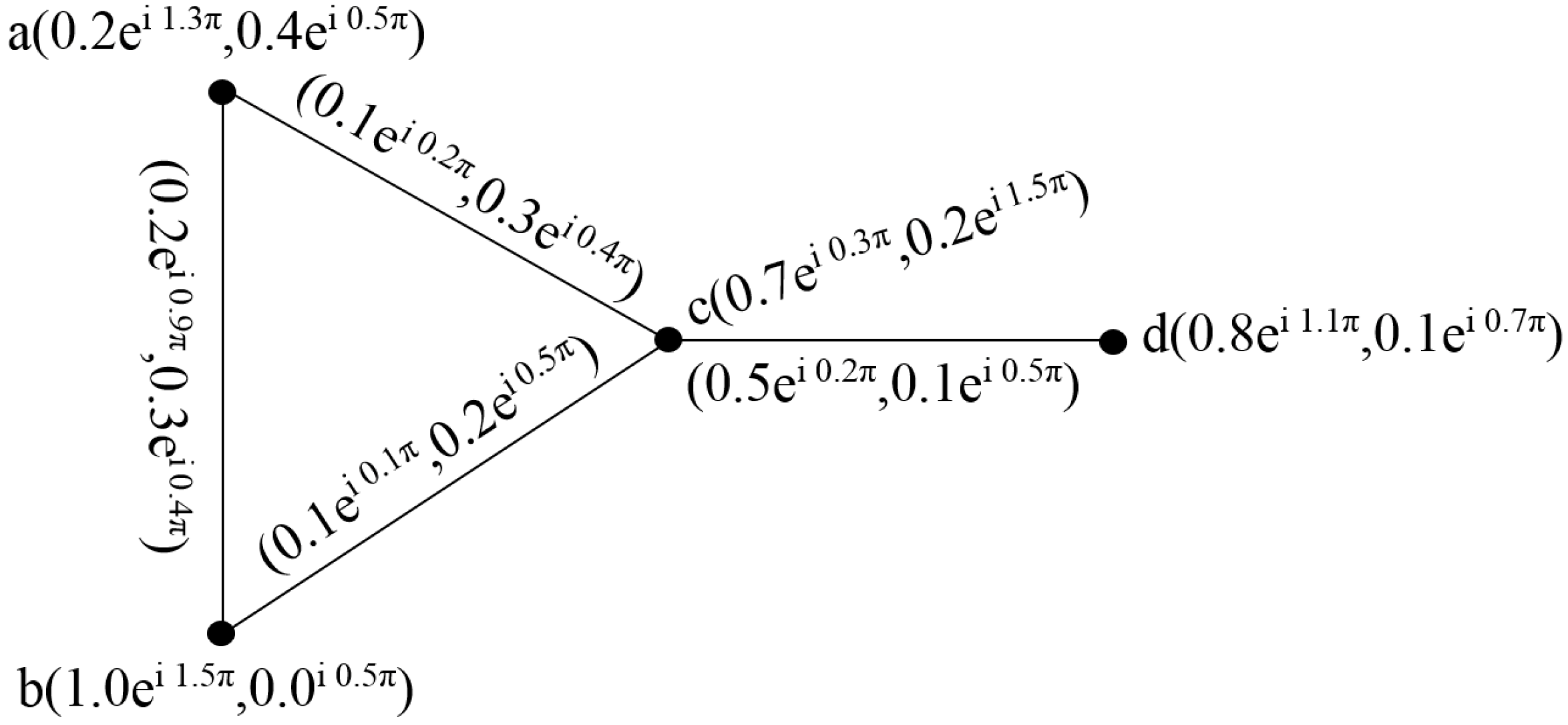
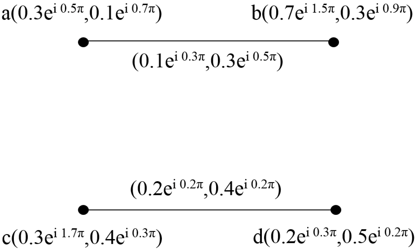
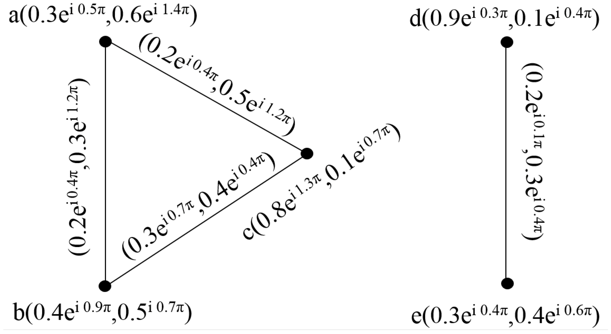
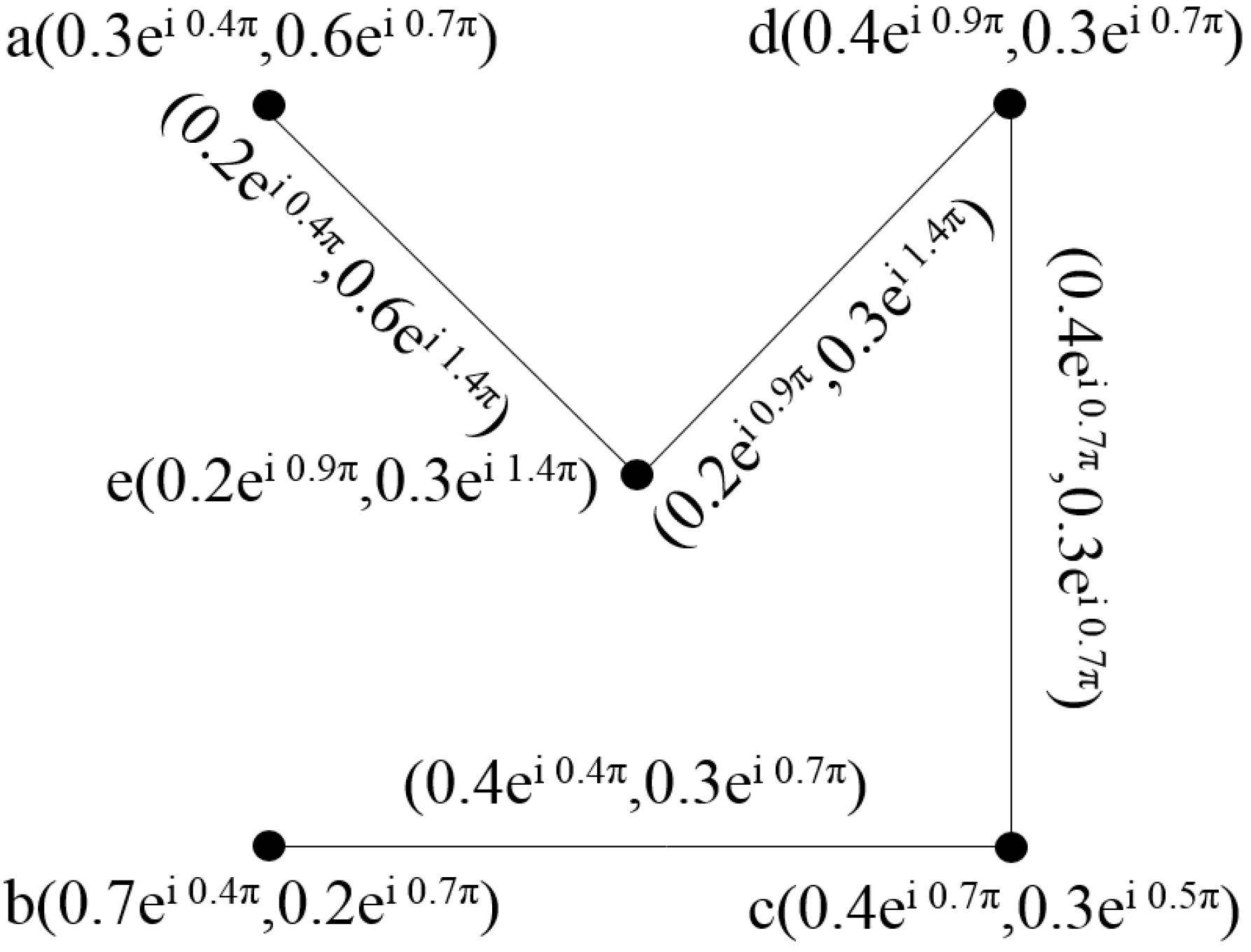
Example 1.

Consider a graph ${\mathbb{G}}^{\ast }=(V,E)$ such that $V=\{a,b,c,d\},$ $E=\{ab,ac,bc,cd\}$. Let $\mathcal{A}$ be a cif-subset of V and let $\mathcal{B}$ be a cif-subset of $E\subseteq V\times V,$ as given:

$$\mathcal{A}=\left(\frac{(0.2e^{i1.3\pi },0.4e^{i0.5\pi })}{a},\frac{(1.0e^{i1.5\pi },0.0e^{i0.5\pi })}{b},\frac{(0.7e^{i0.3\pi },0.2e^{i1.5\pi })}{c},\frac{(0.8e^{i1.1\pi },0.1e^{i0.7\pi })}{d}\right).$$

$$\mathcal{B}=\left(\frac{(0.2e^{i0.9\pi },0.3e^{i0.4\pi })}{ab},\frac{(0.1e^{i0.2\pi },0.3e^{i0.9\pi })}{ac},\frac{(0.1e^{i0.1\pi },0.2e^{i0.5\pi })}{bc},\frac{(0.5e^{i0.2\pi },0.1e^{i0.5\pi })}{cd}\right).$$

(i) 

By routine calculations, it can be observed that the graph shown in Figure 1 is a cif-graph.

(ii) 

Order of cif-graph $=O\left(\mathbb{G}\right)=(2.7e^{i4.2\pi },0.7e^{i3.2\pi })$

(iii) 

Degree of each vertex in $\mathbb{G}$ is

$$\begin{array}{cc}\hfill deg\left(a\right)& =(0.3e^{i1.1\pi },0.6e^{i1.3\pi }),\hfill \\ \hfill deg\left(b\right)& =(0.3e^{i1.0\pi },0.5e^{i0.9\pi }),\hfill \\ \hfill deg\left(c\right)& =(0.7e^{i0.5\pi },0.6e^{i1.9\pi }),\hfill \\ \hfill deg\left(d\right)& =(0.5e^{i0.2\pi },0.1e^{i0.5\pi }).\hfill \end{array}$$

Definition 8.

The Cartesian product ${\mathbb{G}}_1\times {\mathbb{G}}_2$ of two cif-graphs is defined as a pair ${\mathbb{G}}_1\times {\mathbb{G}}_2=({\mathcal{A}}_1\times {\mathcal{A}}_2,{\mathcal{B}}_1\times {\mathcal{B}}_2)$, such that:

1. 

${\mu }_{{\mathcal{A}}_1\times {\mathcal{A}}_2}(x_1,x_2)e^{i{\alpha }_{{\mathcal{A}}_1\times {\mathcal{A}}_2}(x_1,x_2)}=min\{{\mu }_{{\mathcal{A}}_1}\left(x_1\right),{\mu }_{{\mathcal{A}}_2}\left(x_2\right))\}{e}^{i min\{{\alpha }_{{\mathcal{A}}_1}\left(x_1\right),{\alpha }_{{\mathcal{A}}_2}\left(x_2\right)\}}$

${\upsilon }_{{\mathcal{A}}_1\times {\mathcal{A}}_2}(x_1,x_2)e^{i{\beta }_{{\mathcal{A}}_1\times {\mathcal{A}}_2}(x_1,x_2)}=max\{{\upsilon }_{{\mathcal{A}}_1}\left(x_1\right),{\upsilon }_{{\mathcal{A}}_2}\left(x_2\right))\}{e}^{i max\{{\beta }_{{\mathcal{A}}_1}\left(x_1\right),{\beta }_{{\mathcal{A}}_2}\left(x_2\right)\}}$ for all $x_1,x_2\in V,$

2. 

${\mu }_{{\mathcal{B}}_1\times {\mathcal{B}}_2}\left((x,x_2)(x,y_2)\right)e^{i{\alpha }_{{\mathcal{B}}_1\times {\mathcal{B}}_2}\left((x,x_2)(x,y_2)\right)}=min\{{\mu }_{{\mathcal{A}}_1}\left(x\right),{\mu }_{{\mathcal{B}}_2}\left(x_2{y}_2\right))\}{e}^{imin\{{\alpha }_{{\mathcal{A}}_1}\left(x\right),{\alpha }_{{\mathcal{B}}_2}\left(x_2{y}_2\right)\}}$

${\upsilon }_{{\mathcal{B}}_1\times {\mathcal{B}}_2}\left((x,x_2)(x,y_2)\right)e^{i{\beta }_{{\mathcal{B}}_1\times {\mathcal{B}}_2}\left((x,x_2)(x,y_2)\right)}=max\{{\upsilon }_{{\mathcal{A}}_1}\left(x\right),{\upsilon }_{{\mathcal{B}}_2}\left(x_2{y}_2\right))\}{e}^{i max\{{\beta }_{{\mathcal{A}}_1}\left(x\right),{\beta }_{{\mathcal{B}}_2}\left(x_2{y}_2\right)\}}$for all $x\in V_1$, and $x_2{y}_2\in E_2$,

3. 

${\mu }_{{\mathcal{B}}_1\times {\mathcal{B}}_2}\left((x_1,z)(y_1,z)\right)e^{i{\alpha }_{{\mathcal{B}}_1\times {\mathcal{B}}_2}\left((x_1,z)(y_1,z)\right)}=min\{{\mu }_{{\mathcal{B}}_1}\left(x_1{y}_1\right),{\mu }_{{\mathcal{A}}_2}\left(z\right))\}{e}^{i min\{{\alpha }_{{\mathcal{B}}_1}\left(x_1{y}_1\right),{\alpha }_{{\mathcal{A}}_2}\left(z\right)\}}$

${\upsilon }_{{\mathcal{B}}_1\times {\mathcal{B}}_2}\left((x_1,z)(y_1,z)\right)e^{i{\beta }_{{\mathcal{B}}_1\times {\mathcal{B}}_2}\left((x_1,z)(y_1,z)\right)}=max\{{\upsilon }_{{\mathcal{B}}_1}\left(x_1{y}_1\right),{\upsilon }_{{\mathcal{A}}_2}\left(z\right))\}{e}^{i max\{{\beta }_{{\mathcal{B}}_1}\left(x_1{y}_1\right),{\beta }_{{\mathcal{A}}_2}\left(z\right)\}}$for all $z\in V_2$, and $x_1{y}_1\in E_1$.

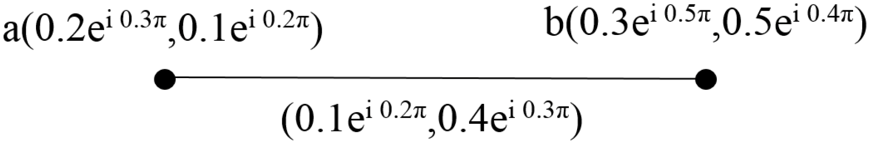
Definition 9.

Let ${\mathbb{G}}_1$ and ${\mathbb{G}}_2$ be two cif-graphs. The degree of a vertex in ${\mathbb{G}}_1\times {\mathbb{G}}_2$ can be defined as follows: for any $(x_1,x_2)\in V_1\times V_2$,

$$d_{{\mathbb{G}}_1\times {\mathbb{G}}_2}(x_1,x_2)=\left(\begin{array}{c}\underset{(x_1,x_2)(y_1,y_2)\in E}{\mathsf{\Sigma }}{\mu }_{{\mathcal{B}}_1\times {\mathcal{B}}_2}\left((x_1,x_2)(y_1,y_2)\right)e^{\underset{(x_1,x_2)(y_1,y_2)\in E}{\mathsf{\Sigma }}{\alpha }_{{\mathcal{B}}_1\times {\mathcal{B}}_2}\left((x_1,x_2)(y_1,y_2)\right)},\\ \underset{(x_1,x_2)(y_1,y_2)\in E}{\mathsf{\Sigma }}{\upsilon }_{{\mathcal{B}}_1\times {\mathcal{B}}_2}\left((x_1,x_2)(y_1,y_2)\right)e^{\underset{(x_1,x_2)(y_1,y_2)\in E}{\mathsf{\Sigma }}{\beta }_{{\mathcal{B}}_1\times {\mathcal{B}}_2}\left((x_1,x_2)(y_1,y_2)\right)}\end{array}\right).$$

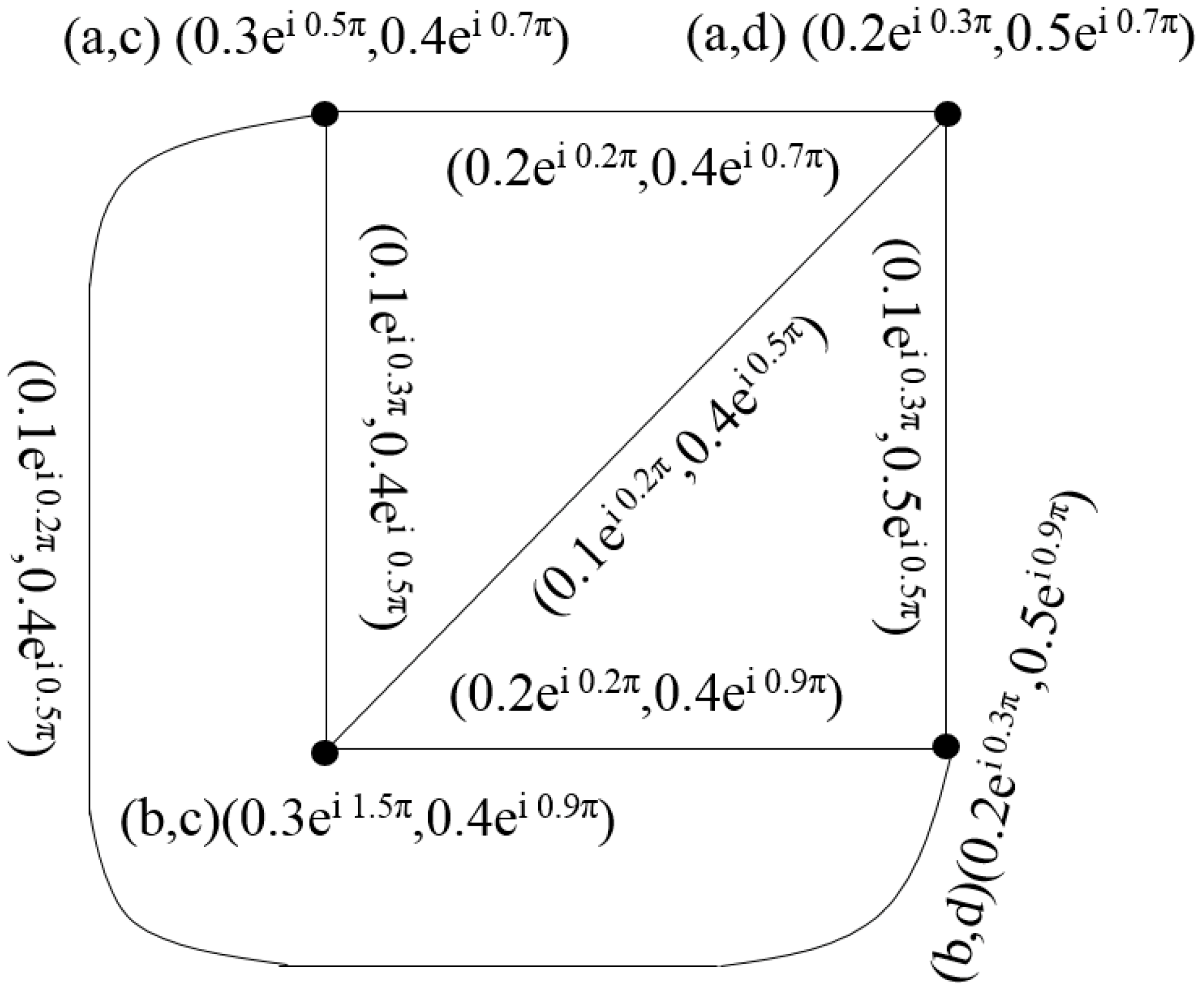
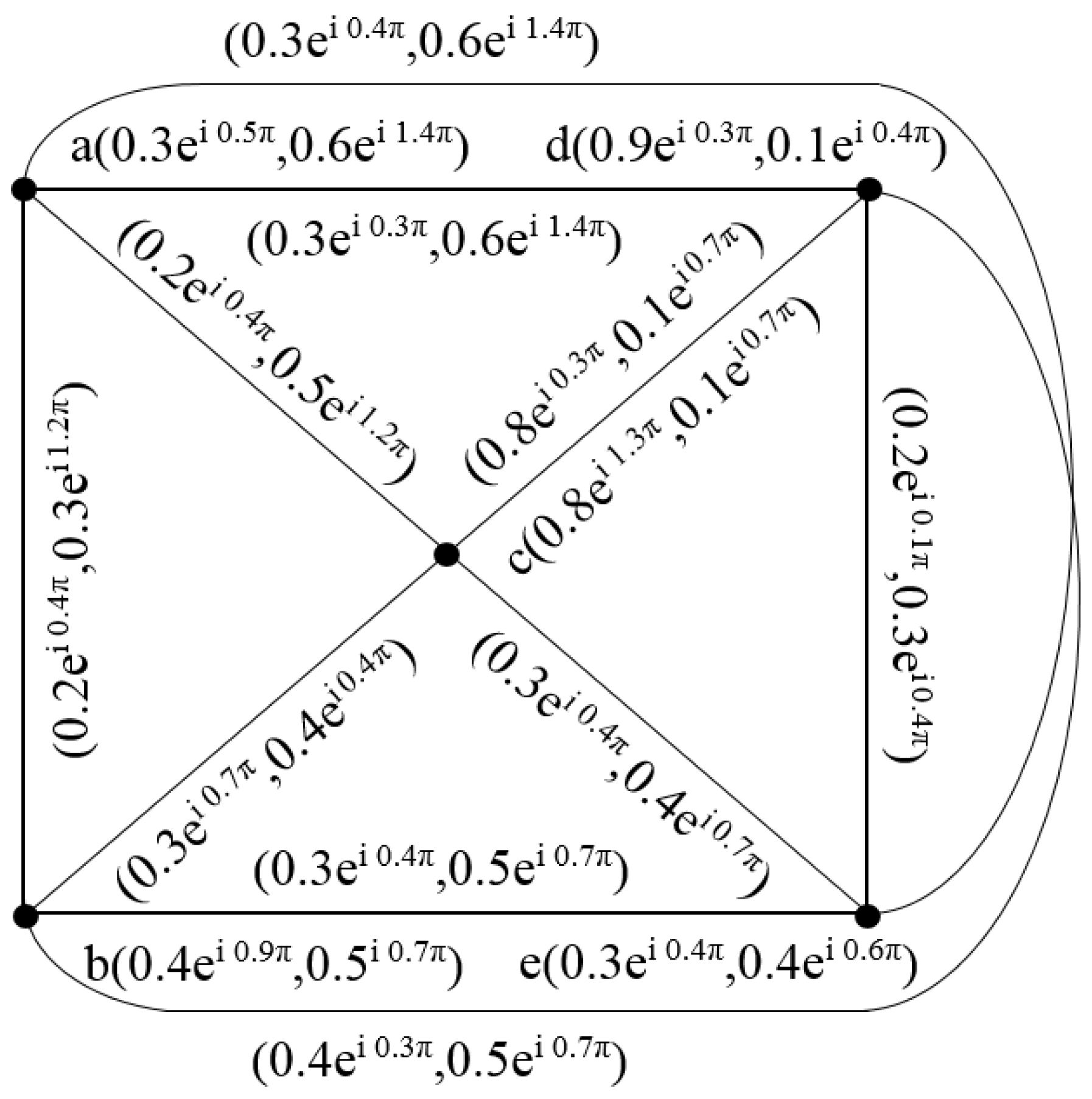
Example 2.

Consider the two cif-graphs ${\mathbb{G}}_1$ and ${\mathbb{G}}_2$, as shown in Figure 2 and Figure 3.

Then, their corresponding Cartesian product ${\mathbb{G}}_1\times {\mathbb{G}}_2$ is shown in Figure 4.

Proposition 1.

The Cartesian product of two cif-graphs is a cif-graph.

Proof. 

The conditions for ${\mathcal{A}}_1\times {\mathcal{A}}_2$ are obvious, therefore, we verify only conditions for ${\mathcal{B}}_1\times {\mathcal{B}}_2$.

Let $x\in V_1$, and $x_2{y}_2\in E_2$. Then,

$$\begin{array}{c}{\mu }_{{\mathcal{B}}_1\times {\mathcal{B}}_2}\left((x,x_2)(x,y_2)\right)e^{i{\alpha }_{{\mathcal{B}}_1\times {\mathcal{B}}_2}\left((x,x_2)(x,y_2)\right)}\hfill \\ =min\{{\mu }_{{\mathcal{A}}_1}\left(x\right),{\mu }_{{\mathcal{B}}_2}\left(x_2{y}_2\right))\}{e}^{imin\{{\alpha }_{{\mathcal{A}}_1}\left(x\right),{\alpha }_{{\mathcal{B}}_2}\left(x_2{y}_2\right)\}}\hfill \\ \le min\{{\mu }_{{\mathcal{A}}_1}\left(x\right),min\{{\mu }_{{\mathcal{A}}_2}\left(x_2\right),{\mu }_{{\mathcal{A}}_2}\left(y_2\right)\}\}{e}^{imin\{{\alpha }_{{\mathcal{A}}_1}\left(x\right),min\{{\alpha }_{{\mathcal{A}}_2}\left(x_2\right),{\alpha }_{{\mathcal{A}}_2}\left(y_2\right)\}\}}\hfill \\ =min\{min\{{\mu }_{{\mathcal{A}}_1}\left(x\right),{\mu }_{{\mathcal{A}}_2}\left(x_2\right)\},min\{{\mu }_{{\mathcal{A}}_1}\left(x\right),{\mu }_{{\mathcal{A}}_2}\left(y_2\right)\}\}{e}^{imin\{min\{{\alpha }_{{\mathcal{A}}_1}\left(x\right),{\alpha }_{{\mathcal{A}}_2}\left(x_2\right)\},min\{{\alpha }_{{\mathcal{A}}_1}\left(x\right),{\alpha }_{{\mathcal{A}}_2}\left(y_2\right)\}\}}\hfill \\ =min\{{\mu }_{{\mathcal{A}}_1\times {\mathcal{A}}_2}(x,x_2),{\mu }_{{\mathcal{A}}_1\times {\mathcal{A}}_2}(x,y_2)\}{e}^{imin\{{\alpha }_{{\mathcal{A}}_1\times {\mathcal{A}}_2}(x,x_2),{\alpha }_{{\mathcal{A}}_1\times {\mathcal{A}}_2}(x,y_2)\}},\hfill \end{array}$$

$$\begin{array}{c}{\upsilon }_{{\mathcal{B}}_1\times {\mathcal{B}}_2}\left((x,x_2)(x,y_2)\right)e^{i{\gamma }_{{\mathcal{B}}_1\times {\mathcal{B}}_2}\left((x,x_2)(x,y_2)\right)}\hfill \\ =max\{{\upsilon }_{{\mathcal{A}}_1}\left(x\right),{\upsilon }_{{\mathcal{B}}_2}\left(x_2{y}_2\right))\}{e}^{imax\{{\gamma }_{{\mathcal{A}}_1}\left(x\right),{\gamma }_{{\mathcal{B}}_2}\left(x_2{y}_2\right)\}}\hfill \\ \le max\{{\upsilon }_{{\mathcal{A}}_1}\left(x\right),max\{{\upsilon }_{{\mathcal{A}}_2}\left(x_2\right),{\upsilon }_{{\mathcal{A}}_2}\left(y_2\right)\}\}{e}^{i max\{{\gamma }_{{\mathcal{A}}_1}\left(x\right),max\{{\gamma }_{{\mathcal{A}}_2}\left(x_2\right),{\gamma }_{{\mathcal{A}}_2}\left(y_2\right)\}\}}\hfill \\ =max\{max\{{\upsilon }_{{\mathcal{A}}_1}\left(x\right),{\upsilon }_{{\mathcal{A}}_2}\left(x_2\right)\},max\{{\upsilon }_{{\mathcal{A}}_1}\left(x\right),{\upsilon }_{{\mathcal{A}}_2}\left(y_2\right)\}\}{e}^{i max\{max\{{\gamma }_{{\mathcal{A}}_1}\left(x\right),{\gamma }_{{\mathcal{A}}_2}\left(x_2\right)\},max\{{\gamma }_{{\mathcal{A}}_1}\left(x\right),{\gamma }_{{\mathcal{A}}_2}\left(y_2\right)\}\}}\hfill \\ =max\{{\upsilon }_{{\mathcal{A}}_1\times {\mathcal{A}}_2}(x,x_2),{\upsilon }_{{\mathcal{A}}_1\times {\mathcal{A}}_2}(x,y_2)\}{e}^{imax\{{\gamma }_{{\mathcal{A}}_1\times {\mathcal{A}}_2}(x,x_2),{\gamma }_{{\mathcal{A}}_1\times {\mathcal{A}}_2}(x,y_2)\}},\hfill \end{array}$$

Similarly, we can prove it for $z\in V_2$ and $x_1{y}_1\in E_1.$  □

Definition 10.

The composition ${\mathbb{G}}_1\circ {\mathbb{G}}_2$ of two $cif$-graphs is defined as a pair ${\mathbb{G}}_1\circ {\mathbb{G}}_2=({\mathcal{A}}_1\circ {\mathcal{A}}_2$, ${\mathcal{B}}_1\circ {\mathcal{B}}_2)$, such that:

1. 

${\mu }_{{\mathcal{A}}_1\circ {\mathcal{A}}_2}(x_1,x_2)e^{i{\alpha }_{{\mathcal{A}}_1\circ {\mathcal{A}}_2}(x_1,x_2)}=min\{{\mu }_{{\mathcal{A}}_1}\left(x_1\right),{\mu }_{{\mathcal{A}}_2}\left(x_2\right))\}{e}^{imin\{{\alpha }_{{\mathcal{A}}_1}\left(x_1\right),{\alpha }_{{\mathcal{A}}_2}\left(x_2\right)\}}$

${\upsilon }_{{\mathcal{A}}_1\circ {\mathcal{A}}_2}(x_1,x_2)e^{i{\beta }_{{\mathcal{A}}_1\circ {\mathcal{A}}_2}(x_1,x_2)}=max\{{\upsilon }_{{\mathcal{A}}_1}\left(x_1\right),{\upsilon }_{{\mathcal{A}}_2}\left(x_2\right))\}{e}^{imax\{{\beta }_{{\mathcal{A}}_1}\left(x_1\right),{\beta }_{{\mathcal{A}}_2}\left(x_2\right)\}}$ for all $x_1$, $x_2\in V$,

2. 

${\mu }_{{\mathcal{B}}_1\circ {\mathcal{B}}_2}\left((x,x_2)(x,y_2)\right)e^{i{\alpha }_{{\mathcal{B}}_1\circ {\mathcal{B}}_2}\left((x,x_2)(x,y_2)\right)}=min\{{\mu }_{{\mathcal{A}}_1}\left(x\right),{\mu }_{{\mathcal{B}}_2}\left(x_2{y}_2\right))\}{e}^{imin\{{\alpha }_{{\mathcal{A}}_1}\left(x\right),{\alpha }_{{\mathcal{B}}_2}\left(x_2{y}_2\right)\}}$

${\upsilon }_{{\mathcal{B}}_1\circ {\mathcal{B}}_2}\left((x,x_2)(x,y_2)\right)e^{i{\beta }_{{\mathcal{B}}_1\circ {\mathcal{B}}_2}\left((x,x_2)(x,y_2)\right)}=max\{{\upsilon }_{{\mathcal{A}}_1}\left(x\right),{\upsilon }_{{\mathcal{B}}_2}\left(x_2{y}_2\right))\}{e}^{imax\{{\beta }_{{\mathcal{A}}_1}\left(x\right),{\beta }_{{\mathcal{B}}_2}\left(x_2{y}_2\right)\}}$

for all $x\in V_1$, and $x_2{y}_2\in E_2$,

3. 

${\mu }_{{\mathcal{B}}_1\circ {\mathcal{B}}_2}\left((x_1,z)(y_1,z)\right)e^{i{\alpha }_{{\mathcal{B}}_1\circ {\mathcal{B}}_2}\left((x_1,z)(y_1,z)\right)}=min\{{\mu }_{{\mathcal{B}}_1}\left(x_1{y}_1\right),{\mu }_{{\mathcal{A}}_2}\left(z\right))\}{e}^{imin\{{\alpha }_{{\mathcal{B}}_1}\left(x_1{y}_1\right),{\alpha }_{{\mathcal{A}}_2}\left(z\right)\}}$

${\upsilon }_{{\mathcal{B}}_1\circ {\mathcal{B}}_2}\left((x_1,z)(y_1,z)\right)e^{i{\beta }_{{\mathcal{B}}_1\circ {\mathcal{B}}_2}\left((x_1,z)(y_1,z)\right)}=max\{{\upsilon }_{{\mathcal{B}}_1}\left(x_1{y}_1\right),{\upsilon }_{{\mathcal{A}}_2}\left(z\right))\}{e}^{imax\{{\beta }_{{\mathcal{B}}_1}\left(x_1{y}_1\right),{\beta }_{{\mathcal{A}}_2}\left(z\right)\}}$for all $z\in V_2$, and $x_1{y}_1\in E_1$.

4. 

${\mu }_{{\mathcal{B}}_1\circ {\mathcal{B}}_2}\left((x_1,x_2)(y_1,y_2)\right)e^{i{\alpha }_{{\mathcal{B}}_1\circ {\mathcal{B}}_2}\left((x_1,x_2)(y_1,y_2)\right)}=min\{{\mu }_{{\mathcal{A}}_2}\left(x_2\right),{\mu }_{{\mathcal{A}}_2}\left(y_2\right),{\mu }_{{\mathcal{B}}_1}\left(x_1{y}_1\right)\}{e}^{imin\{{\alpha }_{{\mathcal{A}}_2}\left(x_2\right),{\alpha }_{{\mathcal{A}}_2}\left(y_2\right),{\alpha }_{{\mathcal{B}}_1}\left(x_1{y}_1\right)\}}$

${\upsilon }_{{\mathcal{B}}_1\circ {\mathcal{B}}_2}\left((x_1,x_2)(y_1,y_2)\right)e^{i{\beta }_{{\mathcal{B}}_1\circ {\mathcal{B}}_2}\left((x_1,x_2)(y_1,y_2)\right)}=max\{{\upsilon }_{{\mathcal{A}}_2}\left(x_2\right),{\upsilon }_{{\mathcal{A}}_2}\left(y_2\right),{\upsilon }_{{\mathcal{B}}_1}\left(x_1{y}_1\right)\}{e}^{imax\{{\beta }_{{\mathcal{A}}_2}\left(x_2\right),{\beta }_{{\mathcal{A}}_2}\left(y_2\right),{\beta }_{{\mathcal{B}}_1}\left(x_1{y}_1\right)\}}$for all $x_2,y_2\in V_2$, $x_2\ne y_2$ and $x_1{y}_1\in E_1$.

Definition 11.

Let ${\mathbb{G}}_1$ and ${\mathbb{G}}_2$ be two cif-graphs. The degree of a vertex in ${\mathbb{G}}_1\circ {\mathbb{G}}_2$ can be defined as follows: for any $(x_1,x_2)\in V_1\times V_2$,

$$d_{{\mathbb{G}}_1\circ {\mathbb{G}}_2}(x_1,x_2)=\left(\begin{array}{c}\underset{(x_1,x_2)(y_1,y_2)\in E}{\mathsf{\Sigma }}{\mu }_{{\mathcal{B}}_1\circ {\mathcal{B}}_2}\left((x_1,x_2)(y_1,y_2)\right)e^{\underset{(x_1,x_2)(y_1,y_2)\in E}{\mathsf{\Sigma }}{\alpha }_{{\mathcal{B}}_1\circ {\mathcal{B}}_2}\left((x_1,x_2)(y_1,y_2)\right)},\\ \underset{(x_1,x_2)(y_1,y_2)\in E}{\mathsf{\Sigma }}{\upsilon }_{{\mathcal{B}}_1\circ {\mathcal{B}}_2}\left((x_1,x_2)(y_1,y_2)\right)e^{\underset{(x_1,x_2)(y_1,y_2)\in E}{\mathsf{\Sigma }}{\beta }_{{\mathcal{B}}_1\circ {\mathcal{B}}_2}\left((x_1,x_2)(y_1,y_2)\right)}\end{array}\right).$$

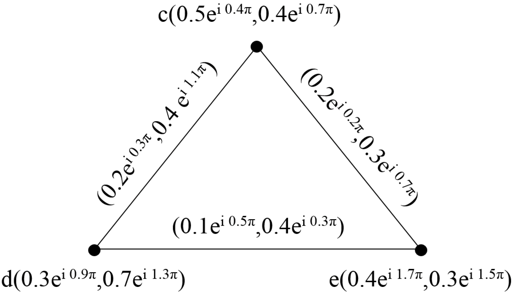
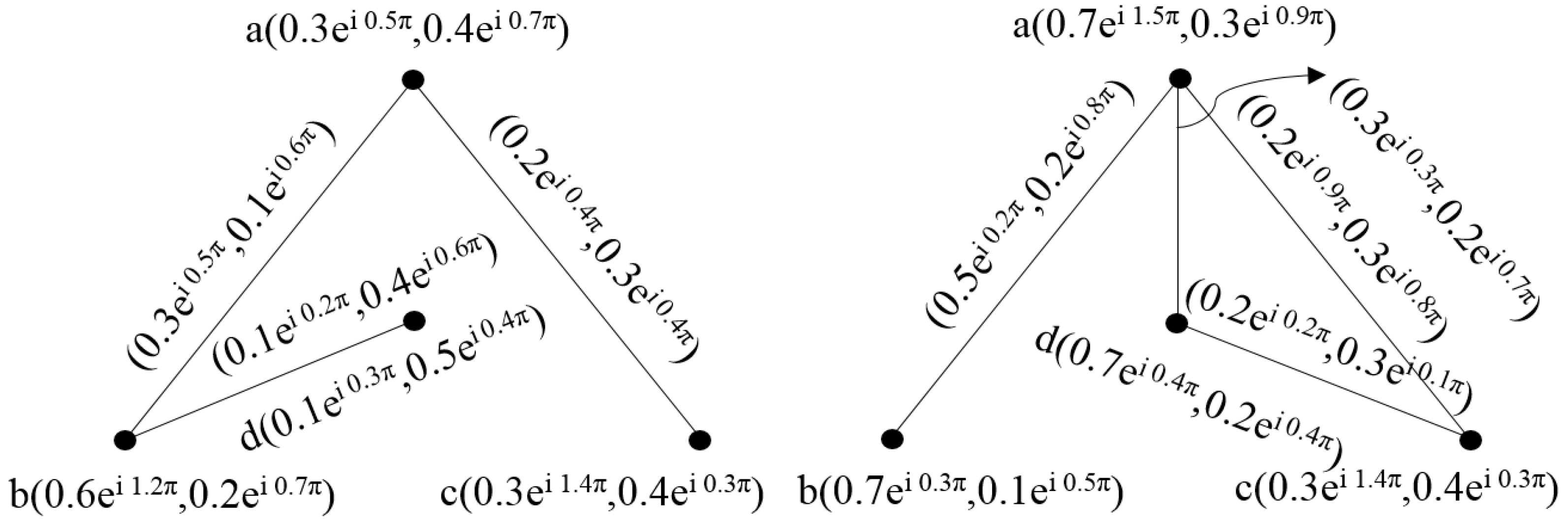
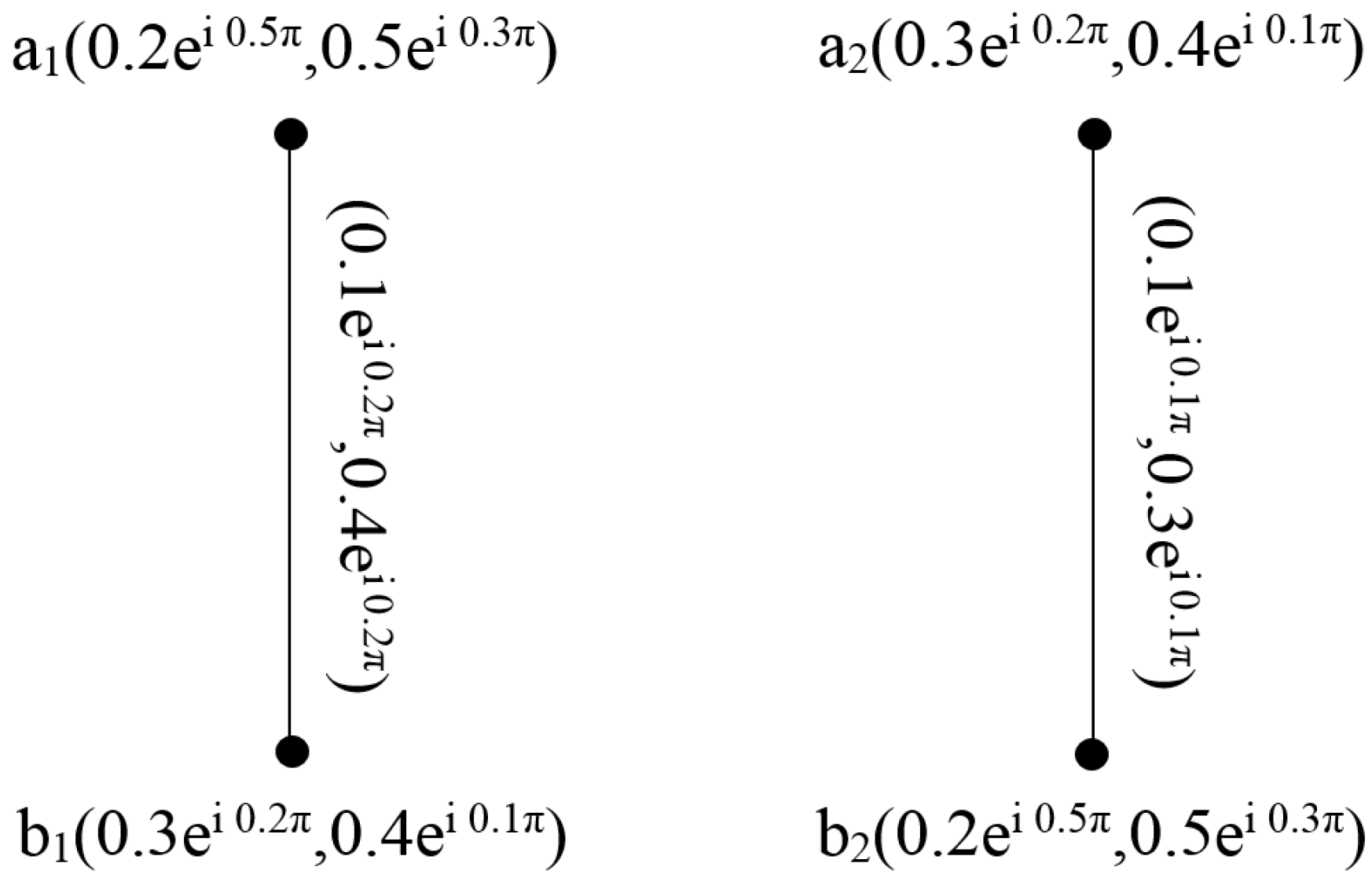
Example 3.

Consider the two cif-graphs, as shown in Figure 5.

Then, their composition ${\mathbb{G}}_1\circ {\mathbb{G}}_2$ is shown in Figure 6.

Proposition 2.

The composition of two cif-graphs is a cif-graph.

Definition 12.

The union ${\mathbb{G}}_1\cup {\mathbb{G}}_2=({\mathcal{A}}_1\cup {\mathcal{A}}_2,{\mathcal{B}}_1\cup {\mathcal{B}}_2)$ of two $cif$-graphs is defined as follows:

1. 

${\mu }_{{\mathcal{A}}_1\cup {\mathcal{A}}_2}\left(x\right)e^{i{\alpha }_{{\mathcal{A}}_1\cup {\mathcal{A}}_2}\left(x\right)}={\mu }_{{\mathcal{A}}_1}\left(x\right)e^{i{\alpha }_{{\mathcal{A}}_1}\left(x\right)},$

${\upsilon }_{{\mathcal{A}}_1\cup {\mathcal{A}}_2}\left(x\right)e^{i{\beta }_{{\mathcal{A}}_1\cup {\mathcal{A}}_2}\left(x\right)}={\upsilon }_{{\mathcal{A}}_1}\left(x\right)e^{i{\beta }_{{\mathcal{A}}_1}\left(x\right)},$ for $x\in V_1$ and $x\notin V_2$.

2. 

${\mu }_{{\mathcal{A}}_1\cup {\mathcal{A}}_2}\left(x\right)e^{i{\alpha }_{{\mathcal{A}}_1\cup {\mathcal{A}}_2}\left(x\right)}={\mu }_{{\mathcal{A}}_2}\left(x\right)e^{i{\alpha }_{{\mathcal{A}}_2}\left(x\right)},$

${\upsilon }_{{\mathcal{A}}_1\cup {\mathcal{A}}_2}\left(x\right)e^{i{\beta }_{{\mathcal{A}}_1\cup {\mathcal{A}}_2}\left(x\right)}={\upsilon }_{{\mathcal{A}}_2}\left(x\right)e^{i{\beta }_{{\mathcal{A}}_2}\left(x\right)},$ for $x\in V_2$ and $x\notin V_1$.

3. 

${\mu }_{{\mathcal{A}}_1\cup {\mathcal{A}}_2}\left(x\right)e^{i{\alpha }_{{\mathcal{A}}_1\cup {\mathcal{A}}_2}\left(x\right)}=max\{{\mu }_{{\mathcal{A}}_1}\left(x\right),{\mu }_{{\mathcal{A}}_2}\left(x\right)\}{e}^{imax\{{\alpha }_{{\mathcal{A}}_1}\left(x\right),{\alpha }_{{\mathcal{A}}_2}\left(x\right)\}},$

${\upsilon }_{{\mathcal{A}}_1\cup {\mathcal{A}}_2}\left(x\right)e^{i{\beta }_{{\mathcal{A}}_1\cup {\mathcal{A}}_2}\left(x\right)}=min\{{\upsilon }_{{\mathcal{A}}_1}\left(x\right),{\upsilon }_{{\mathcal{A}}_2}\left(x\right)\}{e}^{imin\{{\beta }_{{\mathcal{A}}_1}\left(x\right),{\beta }_{{\mathcal{A}}_2}\left(x\right)\}},$ for $x\in V_1\cap V_2$.

4. 

${\mu }_{{\mathcal{B}}_1\cup {\mathcal{B}}_2}\left(xy\right)e^{i{\alpha }_{{\mathcal{B}}_1\cup {\mathcal{B}}_2}\left(xy\right)}={\mu }_{{\mathcal{B}}_1}\left(xy\right)e^{i{\alpha }_{{\mathcal{B}}_1}\left(xy\right)},$

${\upsilon }_{{\mathcal{B}}_1\cup {\mathcal{B}}_2}\left(xy\right)e^{i{\beta }_{{\mathcal{B}}_1\cup {\mathcal{B}}_2}\left(xy\right)}={\upsilon }_{{\mathcal{B}}_1}\left(xy\right)e^{i{\beta }_{{\mathcal{B}}_1}\left(xy\right)},$ for $xy\in E_1$ and $xy\notin E_2$.

5. 

${\mu }_{{\mathcal{B}}_1\cup {\mathcal{B}}_2}\left(xy\right)e^{i{\alpha }_{{\mathcal{B}}_1\cup {\mathcal{B}}_2}\left(xy\right)}={\mu }_{{\mathcal{B}}_2}\left(xy\right)e^{i{\alpha }_{{\mathcal{B}}_2}\left(xy\right)},$

${\upsilon }_{{\mathcal{B}}_1\cup {\mathcal{B}}_2}\left(xy\right)e^{i{\beta }_{{\mathcal{B}}_1\cup {\mathcal{B}}_2}\left(xy\right)}={\upsilon }_{{\mathcal{B}}_2}\left(xy\right)e^{i{\beta }_{{\mathcal{B}}_2}\left(xy\right)},$ for $xy\in V_2$ and $xy\notin V_1$.

6. 

${\mu }_{{\mathcal{B}}_1\cup {\mathcal{B}}_2}\left(xy\right)e^{i{\alpha }_{{\mathcal{B}}_1\cup {\mathcal{B}}_2}\left(xy\right)}=max\{{\mu }_{{\mathcal{B}}_1}\left(xy\right),{\mu }_{{\mathcal{B}}_2}\left(xy\right)\}{e}^{imax\{{\alpha }_{{\mathcal{B}}_1}\left(xy\right),{\alpha }_{{\mathcal{B}}_2}\left(xy\right)\}},$

${\upsilon }_{{\mathcal{B}}_1\cup {\mathcal{B}}_2}\left(xy\right)e^{i{\beta }_{{\mathcal{B}}_1\cup {\mathcal{B}}_2}\left(xy\right)}=min\{{\upsilon }_{{\mathcal{B}}_1}\left(xy\right),{\upsilon }_{{\mathcal{B}}_2}\left(xy\right)\}{e}^{imin\{{\beta }_{{\mathcal{B}}_1}\left(xy\right),{\beta }_{{\mathcal{B}}_2}\left(xy\right)\}},$ for $xy\in V_1\cap V_2$.

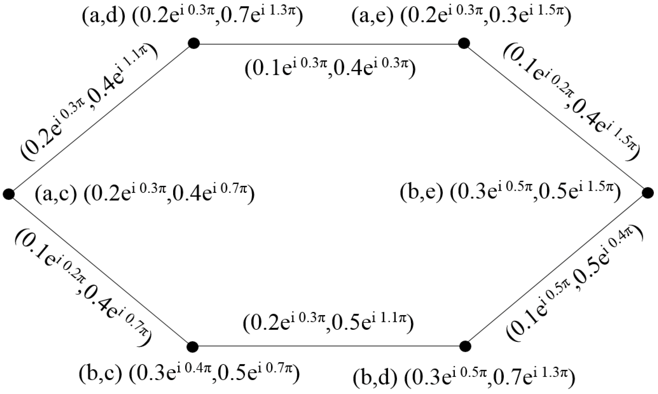
Example 4.

Consider the two cif-graphs, as shown in Figure 7.

Then, their corresponding union ${\mathbb{G}}_1\cup {\mathbb{G}}_2$ is shown in Figure 8.

Proposition 3.

The union of two cif-graphs is a cif-graph.

Definition 13.

The join ${\mathbb{G}}_1+{\mathbb{G}}_2=({\mathcal{A}}_1+{\mathcal{A}}_2,{\mathcal{B}}_1+{\mathcal{B}}_2)$ of two cif-graphs, where $V_1\cap V_2=\varnothing$, is defined as follows:

1. 

$\left\{\begin{array}{l}{\mu }_{{\mathcal{A}}_1+{\mathcal{A}}_2}\left(x\right)e^{i{\alpha }_{{\mathcal{A}}_1+{\mathcal{A}}_2}\left(x\right)}={\mu }_{{\mathcal{A}}_1\cup {\mathcal{A}}_2}\left(x\right)e^{i{\alpha }_{{\mathcal{A}}_1\cup {\mathcal{A}}_2}\left(x\right)}\\ {\upsilon }_{{\mathcal{A}}_1+{\mathcal{A}}_2}\left(x\right)e^{i{\beta }_{{\mathcal{A}}_1+{\mathcal{A}}_2}\left(x\right)}={\upsilon }_{{\mathcal{A}}_1\cup {\mathcal{A}}_2}\left(x\right)e^{i{\beta }_{{\mathcal{A}}_1\cup {\mathcal{A}}_2}\left(x\right)}\end{array}\right.$ if $x\in V_1\cup V_2,$

2. 

$\left\{\begin{array}{l}{\mu }_{{\mathcal{B}}_1+{\mathcal{B}}_2}\left(xy\right)e^{i{\alpha }_{{\mathcal{B}}_1+{\mathcal{B}}_2}\left(x\right)}={\mu }_{{\mathcal{B}}_1\cup {\mathcal{B}}_2}\left(xy\right)e^{i{\alpha }_{{\mathcal{B}}_1\cup {\mathcal{B}}_2}\left(x\right)}\\ {\upsilon }_{{\mathcal{B}}_1+{\mathcal{B}}_2}\left(xy\right)e^{i{\beta }_{{\mathcal{B}}_1+{\mathcal{B}}_2}\left(x\right)}={\upsilon }_{{\mathcal{B}}_1\cup {\mathcal{B}}_2}\left(xy\right)e^{i{\beta }_{{\mathcal{B}}_1\cup {\mathcal{B}}_2}\left(x\right)}\end{array}\right.$ if $xy\in E_1\cap E_2,$

3. 

$\left\{\begin{array}{l}{\mu }_{{\mathcal{B}}_1+{\mathcal{B}}_2}\left(xy\right)e^{i{\alpha }_{{\mathcal{B}}_1+{\mathcal{B}}_2}\left(xy\right)}=min\{{\mu }_{{\mathcal{A}}_1}\left(x\right),{\mu }_{{\mathcal{A}}_2}\left(y\right)\}{e}^{imin\{{\alpha }_{{\mathcal{A}}_1}\left(x\right),{\alpha }_{{\mathcal{A}}_2}\left(y\right)\}}\\ {\upsilon }_{{\mathcal{B}}_1+{\mathcal{B}}_2}\left(xy\right)e^{i{\beta }_{{\mathcal{B}}_1+{\mathcal{B}}_2}\left(xy\right)}=max\{{\upsilon }_{{\mathcal{A}}_1}\left(x\right),{\upsilon }_{{\mathcal{A}}_2}\left(y\right)\}{e}^{imax\{{\beta }_{{\mathcal{A}}_1}\left(x\right),{\beta }_{{\mathcal{A}}_2}\left(y\right)\}}\end{array}\right.$ if $xy\in \acute{E},$ where $\acute{E}$ is the set of all edges joining the vertices of $V_1$ and $V_2$.

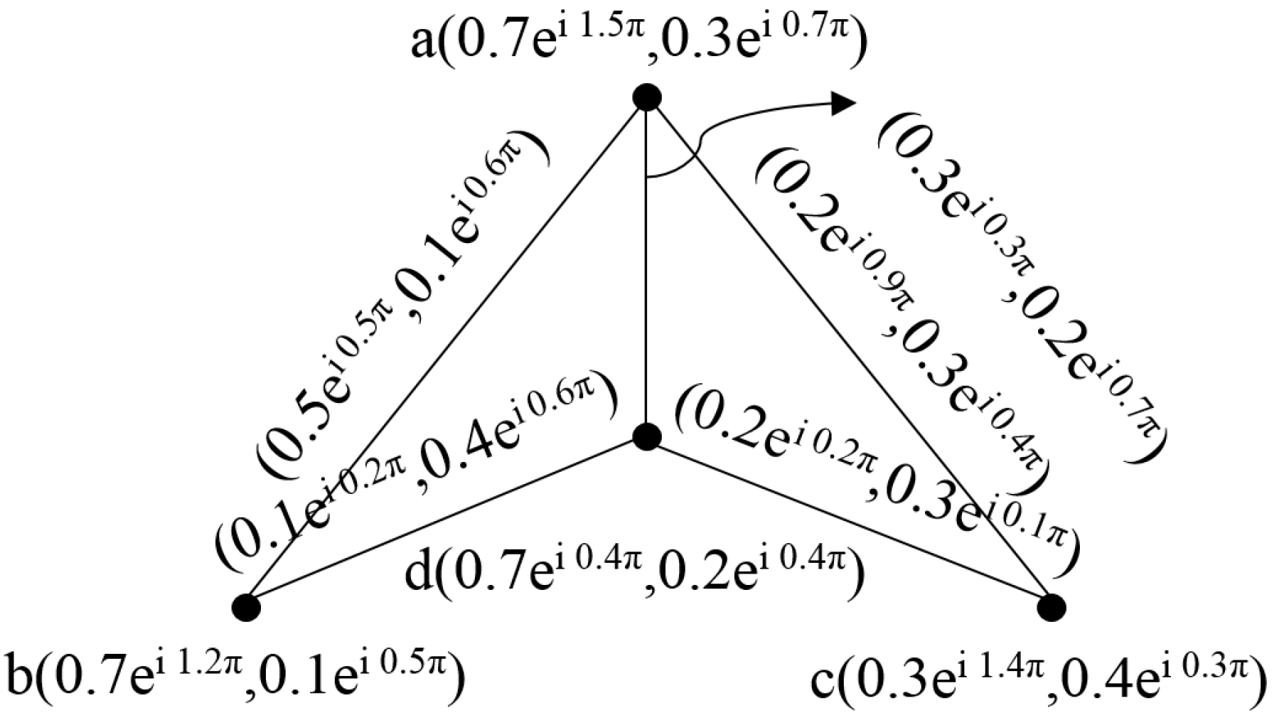
Example 5.

Consider the two cif-graphs, as shown in Figure 9.

Then, their corresponding join ${\mathbb{G}}_1+{\mathbb{G}}_2$ is shown in Figure 10.

Proposition 4.

The join of two cif-graphs is a cif-graph.

Proposition 5.

Let ${\mathbb{G}}_1=({\mathcal{A}}_1,{\mathcal{B}}_1)$ and ${\mathbb{G}}_2=({\mathcal{A}}_2,{\mathcal{B}}_2)$ be cif-graphs of the graphs $G_1^{\ast }$ and $G_2^{\ast }$ and let $V_1\cap V_2=\varnothing .$ Then, union ${\mathbb{G}}_1\cup {\mathbb{G}}_2=({\mathcal{A}}_1\cup {\mathcal{A}}_2,{\mathcal{B}}_1\cup {\mathcal{B}}_2)$ is a cif-graph of $G^{\ast }$ if and only if ${\mathbb{G}}_1$ and ${\mathbb{G}}_2$ are cif-graphs of the graphs $G_1^{\ast }$ and $G_2^{\ast }$, respectively.

Proof. 

Suppose that ${\mathbb{G}}_1\cup {\mathbb{G}}_2$ is a cif-graph. Let $xy\in E_1.$ Then, $xy\notin E_2$ and $x,y\in V_1-V_2.$ Thus,

$$\begin{array}{cc}\hfill {\mu }_{{\mathcal{B}}_1}\left(xy\right)e^{i{\alpha }_{{\mathcal{B}}_1}\left(x\right)}& ={\mu }_{{\mathcal{B}}_1\cap {\mathcal{B}}_2}\left(xy\right)e^{i{\alpha }_{{\mathcal{B}}_1\cap {\mathcal{B}}_2}\left(x\right)}\hfill \\ & \le min({\mu }_{{\mathcal{A}}_1\cap {\mathcal{A}}_2}\left(x\right),{\mu }_{{\mathcal{A}}_1\cap {\mathcal{A}}_2}\left(y\right))e^{imin({\alpha }_{{\mathcal{A}}_1\cap {\mathcal{A}}_2}\left(x\right),{\alpha }_{{\mathcal{A}}_1\cap {\mathcal{A}}_2}\left(y\right))}\hfill \\ & =min({\mu }_{{\mathcal{A}}_1}\left(x\right),{\mu }_{{\mathcal{A}}_1}\left(y\right))e^{imin({\alpha }_{{\mathcal{A}}_1}\left(x\right),{\alpha }_{{\mathcal{A}}_1}\left(y\right))}.\hfill \end{array}$$

$$\begin{array}{cc}\hfill {\upsilon }_{{\mathcal{B}}_1}\left(xy\right)e^{i{\beta }_{{\mathcal{B}}_1}\left(x\right)}& ={\upsilon }_{{\mathcal{B}}_1\cap {\mathcal{B}}_2}\left(xy\right)e^{i{\beta }_{{\mathcal{B}}_1\cap {\mathcal{B}}_2}\left(x\right)}\hfill \\ & \le max({\upsilon }_{{\mathcal{A}}_1\cap {\mathcal{A}}_2}\left(x\right),{\upsilon }_{{\mathcal{A}}_1\cap {\mathcal{A}}_2}\left(y\right))e^{imax({\beta }_{{\mathcal{A}}_1\cap {\mathcal{A}}_2}\left(x\right),{\beta }_{{\mathcal{A}}_1\cap {\mathcal{A}}_2}\left(y\right))}\hfill \\ & =max({\upsilon }_{{\mathcal{A}}_1}\left(x\right),{\upsilon }_{{\mathcal{A}}_1}\left(y\right))e^{imax({\beta }_{{\mathcal{A}}_1}\left(x\right),{\beta }_{{\mathcal{A}}_1}\left(y\right))}.\hfill \end{array}$$

This shows that ${\mathbb{G}}_1=({\mathcal{A}}_1,{\mathcal{B}}_1)$ is a cif-graph. Similarly, we can show that ${\mathbb{G}}_2=({\mathcal{A}}_2,{\mathcal{B}}_2)$ is a cif-graph. The converse part is obvious.  □

Proposition 6.

Let ${\mathbb{G}}_1=({\mathcal{A}}_1,{\mathcal{B}}_1)$ and ${\mathbb{G}}_2=({\mathcal{A}}_2,{\mathcal{B}}_2)$ be cif-graphs of the graphs $G_1^{\ast }$ and $G_2^{\ast }$ and let $V_1\cap V_2=\varnothing .$ Then, join ${\mathbb{G}}_1+{\mathbb{G}}_2=({\mathcal{A}}_1+{\mathcal{A}}_2,{\mathcal{B}}_1+{\mathcal{B}}_2)$ is a cif-graph of $G^{\ast }$ if and only if ${\mathbb{G}}_1$ and ${\mathbb{G}}_2$ are cif-graphs of the graphs $G_1^{\ast }$ and $G_2^{\ast }$, respectively.

Proof. 

The proof is similar to the proof of Proposition 5.  □

4. Isomorphisms of cif-Graphs

In this section, we discuss isomorphisms of cif-graphs.

Definition 14.

Let ${\mathbb{G}}_1=({\mathcal{A}}_1,{\mathcal{B}}_1)$ and ${\mathbb{G}}_2=({\mathcal{A}}_2,{\mathcal{B}}_2)$ be two cif-graphs. A homomorphism $g:{\mathbb{G}}_1\to {\mathbb{G}}_2$ is a mapping $g:V_1\to V_2$ such that:

1. 

$\left\{\begin{array}{l}{\mu }_{{\mathcal{A}}_1}\left(x_1\right)e^{i{\alpha }_{{\mathcal{A}}_1}\left(x_1\right)}\le {\mu }_{{\mathcal{A}}_2}\left(g\left(x_1\right)\right)e^{i{\alpha }_{{\mathcal{A}}_2}\left(g\left(x_1\right)\right)}\\ {\upsilon }_{{\mathcal{A}}_1}\left(x_1\right)e^{i{\beta }_{{\mathcal{A}}_1}\left(x_1\right)}\le {\upsilon }_{{\mathcal{A}}_2}\left(g\left(x_1\right)\right)e^{i{\beta }_{{\mathcal{A}}_2}\left(g\left(x_1\right)\right)}\end{array}\right.$ for all $x_1\in V_1,$

2. 

$\left\{\begin{array}{l}{\mu }_{{\mathcal{B}}_1}\left(x_1{y}_1\right)e^{i{\alpha }_{{\mathcal{B}}_1}\left(x_1{y}_1\right)}\le {\mu }_{{\mathcal{B}}_2}\left(g\left(x_1\right)g\left(y_1\right)\right)e^{i{\alpha }_{{\mathcal{B}}_2}\left(g\left(x_1\right)g\left(y_1\right)\right)}\\ {\upsilon }_{{\mathcal{B}}_1}\left(x_1{y}_1\right)e^{i{\beta }_{{\mathcal{B}}_1}\left(x_1{y}_1\right)}\le {\upsilon }_{{\mathcal{B}}_2}\left(g\left(x_1\right)g\left(y_1\right)\right)e^{i{\beta }_{{\mathcal{B}}_2}\left(g\left(x_1\right)g\left(y_1\right)\right)}\end{array}\right.$ for all $x_1{y}_1\in E_1$.

A bijective homomorphism with the property

3. 

$\left\{\begin{array}{l}{\mu }_{{\mathcal{A}}_1}\left(x_1\right)e^{i{\alpha }_{{\mathcal{A}}_1}\left(x_1\right)}={\mu }_{{\mathcal{A}}_2}\left(g\left(x_1\right)\right)e^{i{\alpha }_{{\mathcal{A}}_2}\left(g\left(x_1\right)\right)}\\ {\upsilon }_{{\mathcal{A}}_1}\left(x_1\right)e^{i{\beta }_{{\mathcal{A}}_1}\left(x_1\right)}={\upsilon }_{{\mathcal{A}}_2}\left(g\left(x_1\right)\right)e^{i{\beta }_{{\mathcal{A}}_2}\left(g\left(x_1\right)\right)}\end{array}\right.$ for all $x_1\in V_1,$ is called a weak isomorphism.

A bijective homomorphism with the property

4. 

$\left\{\begin{array}{l}{\mu }_{{\mathcal{B}}_1}\left(x_1{y}_1\right)e^{i{\alpha }_{{\mathcal{B}}_1}\left(x_1{y}_1\right)}={\mu }_{{\mathcal{B}}_2}\left(g\left(x_1\right)g\left(y_1\right)\right)e^{i{\alpha }_{{\mathcal{B}}_2}\left(g\left(x_1\right)g\left(y_1\right)\right)}\\ {\upsilon }_{{\mathcal{B}}_1}\left(x_1{y}_1\right)e^{i{\beta }_{{\mathcal{B}}_1}\left(x_1{y}_1\right)}={\upsilon }_{{\mathcal{B}}_2}\left(g\left(x_1\right)g\left(y_1\right)\right)e^{i{\beta }_{{\mathcal{B}}_2}\left(g\left(x_1\right)g\left(y_1\right)\right)}\end{array}\right.$ for all $x_1{y}_1\in E_1$, is called a strong co-isomorphism. A bijective mapping $g:{\mathbb{G}}_1\to {\mathbb{G}}_2$ satisfying 3 and 4 is called an isomorphism.

Example 6.

Consider two cif-graphs, as shown in Figure 11.

Then, it is easy to see that the mapping $g:V_1\to V_2$ defined by $g\left(a_1\right)=b_2$ and $g\left(b_1\right)=a_2$ is a weak isomorphism.

Proposition 7.

An isomorphism between cif-graphs is an equivalence relation.

Proof. 

The reflexivity and symmetry are obvious. To prove the transitivity, we let $f:V_1\to V_2$ and $g:V_2\to V_3$ be the isomorphisms of ${\mathbb{G}}_1$ onto ${\mathbb{G}}_2$ and ${\mathbb{G}}_2$ onto ${\mathbb{G}}_3$, respectively. Then, $g\circ f:V_1\to V_3$ is a bijective map from $V_1$ to $V_3$, where $(g\circ f)\left(x_1\right)=g(f$ $\left(x_1\right))$ for all $x_1\in V_1$. Since a map $f:V_1\to V_2$ defined by $f\left(x_1\right)=x_2$ for $x_1\in V_1$ is an isomorphism. Now

$$\begin{array}{cc}\hfill {\mu }_{{\mathcal{A}}_1}\left(x_1\right)e^{i{\alpha }_{{\mathcal{A}}_1}\left(x_1\right)}& ={\mu }_{{\mathcal{A}}_2}\left(f\left(x_1\right)\right)e^{i{\alpha }_{{\mathcal{A}}_2}\left(f\left(x_1\right)\right)}\hfill \\ & ={\mu }_{{\mathcal{A}}_2}\left(x_2\right)e^{i{\alpha }_{{\mathcal{A}}_2}\left(x_2\right)}\mathrm{for}\mathrm{all}{x}_1\in V_1···\left(A_1\right),\hfill \end{array}$$

$$\begin{array}{cc}\hfill {\upsilon }_{{\mathcal{A}}_1}\left(x_1\right)e^{i{\beta }_{{\mathcal{A}}_1}\left(x_1\right)}& ={\upsilon }_{{\mathcal{A}}_2}\left(f\left(x_1\right)\right)e^{i{\beta }_{{\mathcal{A}}_2}\left(f\left(x_1\right)\right)}\hfill \\ & ={\upsilon }_{{\mathcal{A}}_2}\left(x_2\right)e^{i{\beta }_{{\mathcal{A}}_2}\left(x_2\right)}\mathrm{for}\mathrm{all}{x}_1\in V_1···\left(A_2\right),\hfill \end{array}$$

$$\begin{array}{cc}\hfill {\mu }_{{\mathcal{B}}_1}\left(x_1{y}_1\right)e^{i{\alpha }_{{\mathcal{B}}_1}\left(x_1{y}_1\right)}& ={\mu }_{{\mathcal{B}}_2}\left(f\left(x_1\right)f\left(y_1\right)\right)e^{i{\alpha }_{{\mathcal{B}}_2}\left(f\left(x_1\right)f\left(y_1\right)\right)}\hfill \\ & ={\mu }_{{\mathcal{B}}_2}\left(x_2{y}_2\right)e^{i{\alpha }_{{\mathcal{B}}_2}\left(x_2{y}_2\right)}\mathrm{for}\mathrm{all}{x}_1{y}_1\in E_1···\left(B_1\right).\hfill \end{array}$$

$$\begin{array}{cc}\hfill {\upsilon }_{{\mathcal{B}}_1}\left(x_1{y}_1\right)e^{i{\beta }_{{\mathcal{B}}_1}\left(x_1{y}_1\right)}& ={\upsilon }_{{\mathcal{B}}_2}\left(f\left(x_1\right)f\left(y_1\right)\right)e^{i{\beta }_{{\mathcal{B}}_2}\left(f\left(x_1\right)f\left(y_1\right)\right)}\hfill \\ & ={\upsilon }_{{\mathcal{B}}_2}\left(x_2{y}_2\right)e^{i{\beta }_{{\mathcal{B}}_2}\left(x_2{y}_2\right)}\mathrm{for}\mathrm{all}{x}_1{y}_1\in E_1···\left(B_2\right).\hfill \end{array}$$

Since a map $g:V_2\to V_3$ defined by $g\left(x_2\right)=x_3$ for $x_2\in V_2$ is an isomorphism,

$$\begin{array}{cc}\hfill {\mu }_{{\mathcal{A}}_2}\left(x_2\right)e^{i{\alpha }_{{\mathcal{A}}_2}\left(x_2\right)}& ={\mu }_{{\mathcal{A}}_3}\left(g\left(x_2\right)\right)e^{i{\alpha }_{{\mathcal{A}}_3}\left(g\left(x_2\right)\right)}\hfill \\ & ={\mu }_{{\mathcal{A}}_3}\left(x_3\right)e^{i{\alpha }_{{\mathcal{A}}_3}\left(x_3\right)}\mathrm{for}\mathrm{all}{x}_2\in V_2···\left(C_1\right),\hfill \end{array}$$

$$\begin{array}{cc}\hfill {\upsilon }_{{\mathcal{A}}_2}\left(x_2\right)e^{i{\beta }_{{\mathcal{A}}_2}\left(x_2\right)}& ={\upsilon }_{{\mathcal{A}}_3}\left(g\left(x_2\right)\right)e^{i{\beta }_{{\mathcal{A}}_3}\left(g\left(x_2\right)\right)}\hfill \\ & ={\upsilon }_{{\mathcal{A}}_3}\left(x_3\right)e^{i{\beta }_{{\mathcal{A}}_3}\left(x_3\right)}\mathrm{for}\mathrm{all}{x}_2\in V_2···\left(C_2\right),\hfill \end{array}$$

$$\begin{array}{cc}\hfill {\mu }_{{\mathcal{B}}_2}\left(x_2{y}_2\right)e^{i{\alpha }_{{\mathcal{B}}_2}\left(x_2{y}_2\right)}& ={\mu }_{{\mathcal{B}}_3}\left(g\left(x_2\right)g\left(y_2\right)\right)e^{i{\alpha }_{{\mathcal{B}}_3}\left(g\left(x_2\right)g\left(y_2\right)\right)}\hfill \\ & ={\mu }_{{\mathcal{B}}_3}\left(x_3{y}_3\right)e^{i{\alpha }_{{\mathcal{B}}_3}\left(x_3{y}_3\right)}\mathrm{for}\mathrm{all}{x}_2{y}_2\in E_2···\left(D_1\right).\hfill \end{array}$$

$$\begin{array}{cc}\hfill {\upsilon }_{{\mathcal{B}}_2}\left(x_2{y}_2\right)e^{i{\beta }_{{\mathcal{B}}_2}\left(x_2{y}_2\right)}& ={\upsilon }_{{\mathcal{B}}_3}\left(g\left(x_2\right)g\left(y_2\right)\right)e^{i{\beta }_{{\mathcal{B}}_3}\left(g\left(x_2\right)g\left(y_2\right)\right)}\hfill \\ & ={\upsilon }_{{\mathcal{B}}_3}\left(x_3{y}_3\right)e^{i{\beta }_{{\mathcal{B}}_3}\left(x_3{y}_3\right)}\mathrm{for}\mathrm{all}{x}_2{y}_2\in E_2···\left(D_2\right).\hfill \end{array}$$

From $\left(A_1\right),$ $\left(C_1\right)$ and f $\left(x_1\right)=x_2,x_1\in V_1$, we have

$$\begin{array}{cc}\hfill {\mu }_{{\mathcal{A}}_1}\left(x_1\right)e^{i{\alpha }_{{\mathcal{A}}_1}\left(x_1\right)}& ={\mu }_{{\mathcal{A}}_2}\left(f\left(x_1\right)\right)e^{i{\alpha }_{{\mathcal{A}}_2}\left(f\left(x_1\right)\right)}={\mu }_{{\mathcal{A}}_2}\left(x_2\right)e^{i{\alpha }_{{\mathcal{A}}_2}\left(x_2\right)}\hfill \\ & ={\mu }_{{\mathcal{A}}_3}\left(g\left(x_2\right)\right)e^{i{\alpha }_{{\mathcal{A}}_3}\left(g\left(x_2\right)\right)}\hfill \\ & ={\mu }_{{\mathcal{A}}_3}\left(g\left(f\left(x_1\right)\right)\right)e^{i{\alpha }_{{\mathcal{A}}_3}\left(g\left(f\left(x_1\right)\right)\right)}.\hfill \end{array}$$

From $\left(A_2\right),$ $\left(C_2\right)$ and f $\left(x_1\right)=x_2,x_1\in V_1$, we have

$$\begin{array}{cc}\hfill {\upsilon }_{{\mathcal{A}}_1}\left(x_1\right)e^{i{\beta }_{{\mathcal{A}}_1}\left(x_1\right)}& ={\upsilon }_{{\mathcal{A}}_2}\left(f\left(x_1\right)\right)e^{i{\beta }_{{\mathcal{A}}_2}\left(f\left(x_1\right)\right)}={\upsilon }_{{\mathcal{A}}_2}\left(x_2\right)e^{i{\beta }_{{\mathcal{A}}_2}\left(x_2\right)}\hfill \\ & ={\upsilon }_{{\mathcal{A}}_3}\left(g\left(x_2\right)\right)e^{i{\beta }_{{\mathcal{A}}_3}\left(g\left(x_2\right)\right)}\hfill \\ & ={\upsilon }_{{\mathcal{A}}_3}\left(g\left(f\left(x_1\right)\right)\right)e^{i{\beta }_{{\mathcal{A}}_3}\left(g\left(f\left(x_1\right)\right)\right)}.\hfill \end{array}$$

From $\left(B_1\right)$ and $\left(D_1\right)$, we have

$$\begin{array}{cc}\hfill {\mu }_{{\mathcal{B}}_1}\left(x_1{y}_1\right)e^{i{\alpha }_{{\mathcal{B}}_1}\left(x_1{y}_1\right)}& ={\mu }_{{\mathcal{B}}_2}\left(f\left(x_1\right)f\left(y_1\right)\right)e^{i{\alpha }_{{\mathcal{B}}_2}\left(f\left(x_1\right)f\left(y_1\right)\right)}={\mu }_{{\mathcal{B}}_2}\left(x_2{y}_2\right)e^{i{\alpha }_{{\mathcal{B}}_2}\left(x_2{y}_2\right)}\hfill \\ & ={\mu }_{{\mathcal{B}}_3}\left(g\left(x_2\right)g\left(y_2\right)\right)e^{i{\alpha }_{{\mathcal{B}}_3}\left(g\left(x_2\right)g\left(y_2\right)\right)}\hfill \\ & ={\mu }_{{\mathcal{B}}_3}\left(g\left(f\left(x_1\right)\right)g\left(f\left(y_1\right)\right)\right)e^{i{\alpha }_{{\mathcal{B}}_3}\left(g\left(f\left(x_1\right)\right)g\left(f\left(y_1\right)\right)\right)}.\hfill \end{array}$$

From $\left(B_2\right)$ and $\left(D_2\right)$, we have

$$\begin{array}{cc}\hfill {\upsilon }_{{\mathcal{B}}_1}\left(x_1{y}_1\right)e^{i{\beta }_{{\mathcal{B}}_1}\left(x_1{y}_1\right)}& ={\upsilon }_{{\mathcal{B}}_2}\left(f\left(x_1\right)f\left(y_1\right)\right)e^{i{\beta }_{{\mathcal{B}}_2}\left(f\left(x_1\right)f\left(y_1\right)\right)}={\upsilon }_{{\mathcal{B}}_2}\left(x_2{y}_2\right)e^{i{\beta }_{{\mathcal{B}}_2}\left(x_2{y}_2\right)}\hfill \\ & ={\upsilon }_{{\mathcal{B}}_3}\left(g\left(x_2\right)g\left(y_2\right)\right)e^{i{\beta }_{{\mathcal{B}}_3}\left(g\left(x_2\right)g\left(y_2\right)\right)}\hfill \\ & ={\upsilon }_{{\mathcal{B}}_3}\left(g\left(f\left(x_1\right)\right)g\left(f\left(y_1\right)\right)\right)e^{i{\beta }_{{\mathcal{B}}_3}\left(g\left(f\left(x_1\right)\right)g\left(f\left(y_1\right)\right)\right)},\hfill \end{array}$$

for all $x_1{y}_1\in E_1$. Therefore, $g\circ f$ is an isomorphism between ${\mathbb{G}}_1$ and ${\mathbb{G}}_3$. This completes the proof.  □

Proposition 8.

A weak isomorphism (co-isomorphism) between cif-graphs is a partial ordering relation.

Proof. 

The reflexivity and transitivity are obvious. To prove the anti-symmetry, we let $f:V_1\to V_2$ be a strong isomorphism of ${\mathbb{G}}_1$ onto ${\mathbb{G}}_2$. Then, f is a bijective map defined by f $\left(x_1\right)=x_2$ for all $x_1\in V_1$ satisfying

$${\mu }_{{\mathcal{A}}_1}\left(x_1\right)e^{i{\alpha }_{{\mathcal{A}}_1}\left(x_1\right)}={\mu }_{{\mathcal{A}}_2}\left(f\left(x_1\right)\right)e^{i{\alpha }_{{\mathcal{A}}_2}\left(f\left(x_1\right)\right)}\mathrm{for}\mathrm{all}{x}_1\in V_1,$$

$${\upsilon }_{{\mathcal{A}}_1}\left(x_1\right)e^{i{\beta }_{{\mathcal{A}}_1}\left(x_1\right)}={\upsilon }_{{\mathcal{A}}_2}\left(f\left(x_1\right)\right)e^{i{\beta }_{{\mathcal{A}}_2}\left(f\left(x_1\right)\right)}\mathrm{for}\mathrm{all}{x}_1\in V_1,$$

$${\mu }_{{\mathcal{B}}_1}\left(x_1{y}_1\right)e^{i{\alpha }_{{\mathcal{B}}_1}\left(x_1{y}_1\right)}\le {\mu }_{{\mathcal{B}}_2}\left(f\left(x_1\right)f\left(y_1\right)\right)e^{i{\alpha }_{{\mathcal{B}}_2}\left(f\left(x_1\right)f\left(y_1\right)\right)}\mathrm{for}\mathrm{all}{x}_1{y}_1\in E_1···\left(I_1\right).$$

$${\upsilon }_{{\mathcal{B}}_1}\left(x_1{y}_1\right)e^{i{\beta }_{{\mathcal{B}}_1}\left(x_1{y}_1\right)}\le {\upsilon }_{{\mathcal{B}}_2}\left(f\left(x_1\right)f\left(y_1\right)\right)e^{i{\beta }_{{\mathcal{B}}_2}\left(f\left(x_1\right)f\left(y_1\right)\right)}\mathrm{for}\mathrm{all}{x}_1{y}_1\in E_1···\left(I_2\right).$$

Let $g:V_2\to V_1$ be a strong isomorphism of ${\mathbb{G}}_2$ onto ${\mathbb{G}}_1$. Then, g is a bijective map defined by $g\left(x_2\right)=x_1$ for all $x_2\in V_2$ satisfying

$${\mu }_{{\mathcal{A}}_2}\left(x_2\right)e^{i{\alpha }_{{\mathcal{A}}_2}\left(x_2\right)}={\mu }_{{\mathcal{A}}_1}\left(g\left(x_2\right)\right)e^{i{\alpha }_{{\mathcal{A}}_1}\left(g\left(x_2\right)\right)}\mathrm{for}\mathrm{all}{x}_2\in V_2,$$

$${\upsilon }_{{\mathcal{A}}_2}\left(x_2\right)e^{i{\beta }_{{\mathcal{A}}_2}\left(x_2\right)}={\upsilon }_{{\mathcal{A}}_1}\left(g\left(x_2\right)\right)e^{i{\beta }_{{\mathcal{A}}_1}\left(g\left(x_2\right)\right)}\mathrm{for}\mathrm{all}{x}_2\in V_2,$$

$${\mu }_{{\mathcal{B}}_2}\left(x_2{y}_2\right)e^{i{\alpha }_{{\mathcal{B}}_2}\left(x_2{y}_2\right)}\le {\mu }_{{\mathcal{B}}_1}\left(g\left(x_2\right)g\left(y_2\right)\right)e^{i{\alpha }_{{\mathcal{B}}_1}\left(g\left(x_2\right)g\left(y_2\right)\right)}\mathrm{for}\mathrm{all}{x}_2{y}_2\in E_2···\left(J_1\right).$$

$${\upsilon }_{{\mathcal{B}}_2}\left(x_2{y}_2\right)e^{i{\beta }_{{\mathcal{B}}_2}\left(x_2{y}_2\right)}\le {\upsilon }_{{\mathcal{B}}_1}\left(g\left(x_2\right)g\left(y_2\right)\right)e^{i{\beta }_{{\mathcal{B}}_1}\left(g\left(x_2\right)g\left(y_2\right)\right)}\mathrm{for}\mathrm{all}{x}_2{y}_2\in E_2···\left(J_2\right).$$

The inequalities $\left(I_1\right)$, $\left(J_1\right)$ and $\left(I_2\right)$, $\left(J_2\right)$ hold on the finite sets $V_1$ and $V_2$ only when ${\mathbb{G}}_1$ and ${\mathbb{G}}_2$ have the same number of edges and the corresponding edges have same weight. Hence, ${\mathbb{G}}_1$ and ${\mathbb{G}}_2$ are identical. Therefore, $g\circ f$ is a strong isomorphism between ${\mathbb{G}}_1$ and ${\mathbb{G}}_3$. This completes the proof.  □

5. Complement of cif-Graphs

In this section, we discuss complements of cif-graphs.

Definition 15.

The complement of a weak cif-graph $\mathbb{G}=(\mathcal{A},\mathcal{B})$ of $G^{\ast }=(V,E)$ is a weak cif-graph $\overline{\mathbb{G}}=(\overline{\mathcal{A}},\overline{\mathcal{B}})$ on $\overline{G^{\ast }}$, is defined by

(i) 

$\overline{V}=V,$

(ii) 

$\left\{\begin{array}{c}{\mu }_{\overline{\mathcal{A}}}\left(x\right)e^{i{\alpha }_{\overline{\mathcal{A}}}\left(x\right)}={\mu }_{\mathcal{A}}\left(x\right)e^{i{\alpha }_{\mathcal{A}}\left(x\right)}\\ {\upsilon }_{\overline{\mathcal{A}}}\left(x\right)e^{i{\beta }_{\overline{\mathcal{A}}}\left(x\right)}={\upsilon }_{\mathcal{A}}\left(x\right)e^{i{\beta }_{\mathcal{A}}\left(x\right)}\end{array}\right.$ for all $x\in V$,

(iii) 

$\left\{\begin{array}{c}{\mu }_{\overline{\mathcal{B}}}\left(xy\right)e^{i{\alpha }_{\overline{\mathcal{B}}}\left(xy\right)}=\left\{\begin{array}{cc}0\hfill & if {\mu }_{\mathcal{B}}\left(xy\right)e^{i{\alpha }_{\mathcal{B}}\left(xy\right)}\ne 0\\ \hfill min\{{\mu }_{\mathcal{A}}\left(x\right),{\mu }_{\mathcal{A}}\left(y\right)\}{e}^{imin\{{\alpha }_{\mathcal{A}}\left(x\right),{\alpha }_{\mathcal{A}}\left(y\right)\}}& if {\mu }_{\mathcal{B}}\left(xy\right)e^{i{\alpha }_{\mathcal{B}}\left(xy\right)}=0.\end{array}\right.\\ {\upsilon }_{\overline{\mathcal{B}}}\left(xy\right)e^{i{\beta }_{\overline{\mathcal{B}}}\left(xy\right)}=\left\{\begin{array}{cc}0\hfill & if {\upsilon }_{\mathcal{B}}\left(xy\right)e^{i{\beta }_{\mathcal{B}}\left(xy\right)}\ne 0\\ \hfill max\{{\upsilon }_{\mathcal{A}}\left(x\right),{\upsilon }_{\mathcal{A}}\left(y\right)\}{e}^{imax\{{\beta }_{\mathcal{A}}\left(x\right),{\beta }_{\mathcal{A}}\left(y\right)\}}& if {\upsilon }_{\mathcal{B}}\left(xy\right)e^{i{\beta }_{\mathcal{B}}\left(xy\right)}=0.\end{array}\right.\end{array}\right.$

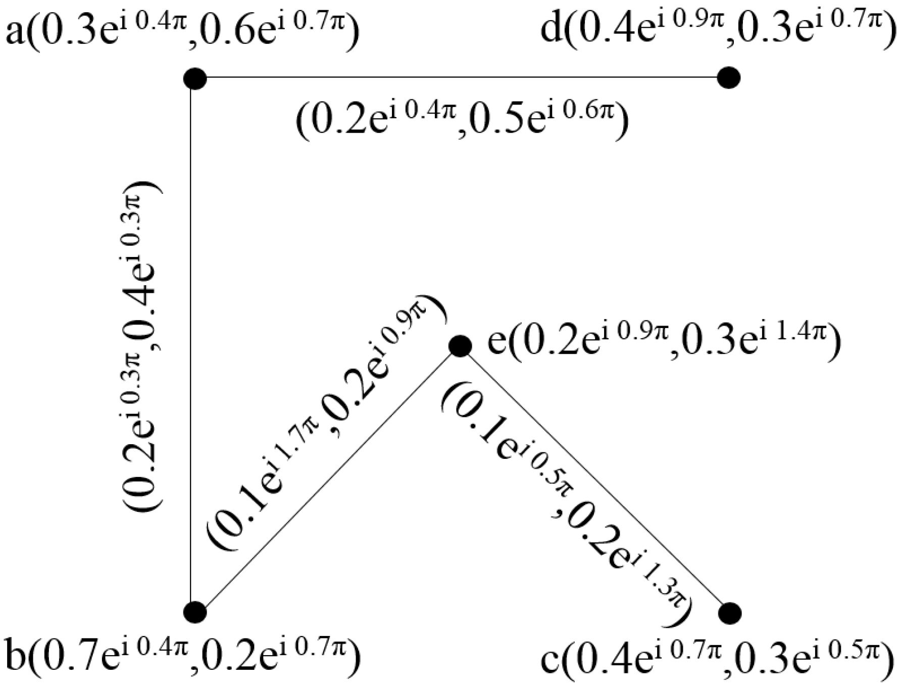
Example 7.

Consider a cif-graph $\mathbb{G}$, as shown in Figure 12.

Then, the complement $\overline{\mathbb{G}}$ of $\mathbb{G}$ is shown in Figure 13.

Definition 16.

A cif-graph G is called self complementary if $\overline{\mathbb{G}}\approx \mathbb{G}$.

The following propositions are obvious.

Proposition 9.

Let $\mathbb{G}=(\mathcal{A},\mathcal{B})$ be a self complementary cif-graph. Then,

$$\begin{array}{cc}\hfill \underset{x\ne y}{\mathsf{\Sigma }}{\mu }_{\mathcal{B}}\left(xy\right)e^{i{\alpha }_{\mathcal{B}}\left(xy\right)}& =\underset{x\ne y}{\mathsf{\Sigma }}min\{{\mu }_{\mathcal{A}}\left(x\right),{\mu }_{\mathcal{A}}\left(y\right)\}{e}^{imin\{{\alpha }_{\mathcal{A}}\left(x\right),{\alpha }_{\mathcal{A}}\left(y\right)\}}\hfill \\ \hfill \underset{x\ne y}{\mathsf{\Sigma }}{\upsilon }_{\mathcal{B}}\left(xy\right)e^{i{\beta }_{\mathcal{B}}\left(xy\right)}& =\underset{x\ne y}{\mathsf{\Sigma }}max\{{\upsilon }_{\mathcal{A}}\left(x\right),{\upsilon }_{\mathcal{A}}\left(y\right)\}{e}^{imax\{{\beta }_{\mathcal{A}}\left(x\right),{\beta }_{\mathcal{A}}\left(y\right)\}}.\hfill \end{array}$$

Proposition 10.

Let $\mathbb{G}=(\mathcal{A},\mathcal{B})$ be a cif-graph. If

$$\begin{array}{cc}\hfill {\mu }_{\mathcal{B}}\left(xy\right)e^{i{\alpha }_{\mathcal{B}}\left(xy\right)}& =min\{{\mu }_{\mathcal{A}}\left(x\right),{\mu }_{\mathcal{A}}\left(y\right)\}{e}^{imin\{{\alpha }_{\mathcal{A}}\left(x\right),{\alpha }_{\mathcal{A}}\left(y\right)\}}\hfill \\ \hfill {\upsilon }_{\mathcal{B}}\left(xy\right)e^{i{\beta }_{\mathcal{B}}\left(xy\right)}& =max\{{\upsilon }_{\mathcal{A}}\left(x\right),{\upsilon }_{\mathcal{A}}\left(y\right)\}{e}^{imax\{{\beta }_{\mathcal{A}}\left(x\right),{\beta }_{\mathcal{A}}\left(y\right)\}},\hfill \end{array}$$

$x,y\in V,$ then G is self complementary.

Proposition 11.

Let ${\mathbb{G}}_1$ and ${\mathbb{G}}_2$ be cif-graphs. If there is a strong isomorphism between ${\mathbb{G}}_1$ and ${\mathbb{G}}_2$, then there is a strong isomorphism between $\overline{{\mathbb{G}}_1}$ and $\overline{{\mathbb{G}}_2}$.

Proof. 

Let f be a strong isomorphism between ${\mathbb{G}}_1$ and ${\mathbb{G}}_2$. Then, $f:V_1\to V_2$ is a bijective map that satisfies

$$f\left(x_1\right)=x_2\mathrm{for}\mathrm{all}{x}_1\in V_1,$$

$$\begin{array}{cc}\hfill {\mu }_{{\mathcal{A}}_1}\left(x_1\right)e^{i{\alpha }_{{\mathcal{A}}_1}\left(x_1\right)}& ={\mu }_{{\mathcal{A}}_2}\left(f\left(x_1\right)\right)e^{i{\alpha }_{{\mathcal{A}}_2}\left(f\left(x_1\right)\right)}\mathrm{for}\mathrm{all}x\in V_1.\hfill \\ \hfill {\upsilon }_{{\mathcal{A}}_1}\left(x_1\right)e^{i{\beta }_{{\mathcal{A}}_1}\left(x_1\right)}& ={\upsilon }_{{\mathcal{A}}_2}\left(f\left(x_1\right)\right)e^{i{\beta }_{{\mathcal{A}}_2}\left(f\left(x_1\right)\right)}\mathrm{for}\mathrm{all}x\in V_1.\hfill \end{array}$$

$$\begin{array}{cc}\hfill {\mu }_{{\mathcal{A}}_1}\left(x_1{y}_1\right)e^{i{\alpha }_{{\mathcal{A}}_1}\left(x_1{y}_1\right)}& \le {\mu }_{{\mathcal{A}}_2}\left(f\left(x_1\right)f\left(y_1\right)\right)e^{i{\alpha }_{{\mathcal{A}}_2}\left(f\left(x_1\right)f\left(y_1\right)\right)}\mathrm{for}\mathrm{all}{x}_1{y}_1\in E_1.\hfill \\ \hfill {\upsilon }_{{\mathcal{A}}_1}\left(x_1{y}_1\right)e^{i{\beta }_{{\mathcal{A}}_1}\left(x_1{y}_1\right)}& \le {\upsilon }_{{\mathcal{A}}_2}\left(f\left(x_1\right)f\left(y_1\right)\right)e^{i{\beta }_{{\mathcal{A}}_2}\left(f\left(x_1\right)f\left(y_1\right)\right)}\mathrm{for}\mathrm{all}{x}_1{y}_1\in E_1.\hfill \end{array}$$

Since $f:V_1\to V_2$ is a bijective map, f ${}^{-1}:V_2\to V_1$ is also bijective map such that f ${}^{-1}\left(x_2\right)=x_1$ for all $x_2\in V_2.$ Thus

$$\begin{array}{cc}\hfill {\mu }_{{\mathcal{A}}_1}\left(f^{-1}\left(x_2\right)\right)e^{i{\alpha }_{{\mathcal{A}}_1}\left(f^{-1}\left(x_2\right)\right)}& ={\mu }_{{\mathcal{A}}_2}\left(x_2\right)e^{i{\alpha }_{{\mathcal{A}}_2}\left(x_2\right)}\mathrm{for}\mathrm{all}{x}_2\in V_2.\hfill \\ \hfill {\upsilon }_{{\mathcal{A}}_1}\left(f^{-1}\left(x_2\right)\right)e^{i{\beta }_{{\mathcal{A}}_1}\left(f^{-1}\left(x_2\right)\right)}& ={\upsilon }_{{\mathcal{A}}_2}\left(x_2\right)e^{i{\beta }_{{\mathcal{A}}_2}\left(x_2\right)}\mathrm{for}\mathrm{all}{x}_2\in V_2.\hfill \end{array}$$

By definition of complement, we have

$$\begin{array}{cc}\hfill {\mu }_{\overline{{\mathcal{B}}_1}}\left(x_1{y}_1\right)e^{i{\alpha }_{\overline{{\mathcal{B}}_1}}\left(x_1{y}_1\right)}& =min\{{\mu }_{{\mathcal{A}}_1}\left(x_1\right),{\mu }_{{\mathcal{A}}_1}\left(y_1\right)\}{e}^{imin\{{\alpha }_{{\mathcal{A}}_1}\left(x_1\right),{\alpha }_{{\mathcal{A}}_1}\left(y_1\right)\}}\hfill \\ & \le min\{{\mu }_{{\mathcal{A}}_2}\left(f\left(x_2\right)\right),{\mu }_{{\mathcal{A}}_2}\left(f\left(y_2\right)\right)\}{e}^{imin\{{\alpha }_{{\mathcal{A}}_2}\left(f\left(x_2\right)\right),{\alpha }_{{\mathcal{A}}_2}\left(f\left(y_2\right)\right)\}}\hfill \\ & =min\{{\mu }_{{\mathcal{A}}_2}\left(x_2\right),{\mu }_{{\mathcal{A}}_2}\left(y_2\right)\}{e}^{imin\{{\alpha }_{{\mathcal{A}}_2}\left(x_2\right),{\alpha }_{{\mathcal{A}}_2}\left(y_2\right)\}}\hfill \\ & ={\mu }_{{\mathcal{B}}_2}\left(x_2{y}_2\right)e^{i{\alpha }_{{\mathcal{B}}_2}\left(x_2{y}_2\right)}.\hfill \end{array}$$

$$\begin{array}{cc}\hfill {\upsilon }_{\overline{{\mathcal{B}}_1}}\left(x_1{y}_1\right)e^{i{\beta }_{\overline{{\mathcal{B}}_1}}\left(x_1{y}_1\right)}& =max\{{\upsilon }_{{\mathcal{A}}_1}\left(x_1\right),{\upsilon }_{{\mathcal{A}}_1}\left(y_1\right)\}{e}^{imax\{{\beta }_{{\mathcal{A}}_1}\left(x_1\right),{\beta }_{{\mathcal{A}}_1}\left(y_1\right)\}}\hfill \\ & \le max\{{\upsilon }_{{\mathcal{A}}_2}\left(f\left(x_2\right)\right),{\upsilon }_{{\mathcal{A}}_2}\left(f\left(y_2\right)\right)\}{e}^{imax\{{\beta }_{{\mathcal{A}}_2}\left(f\left(x_2\right)\right),{\beta }_{{\mathcal{A}}_2}\left(f\left(y_2\right)\right)\}}\hfill \\ & =max\{{\upsilon }_{{\mathcal{A}}_2}\left(x_2\right),{\upsilon }_{{\mathcal{A}}_2}\left(y_2\right)\}{e}^{imax\{{\beta }_{{\mathcal{A}}_2}\left(x_2\right),{\beta }_{{\mathcal{A}}_2}\left(y_2\right)\}}\hfill \\ & ={\upsilon }_{{\mathcal{B}}_2}\left(x_2{y}_2\right)e^{i{\beta }_{{\mathcal{B}}_2}\left(x_2{y}_2\right)}.\hfill \end{array}$$

Thus, f ${}^{-1}:V_2\to V_1$ is a bijective map which is a strong isomorphism between $\overline{{\mathbb{G}}_1}$ and $\overline{{\mathbb{G}}_2}$. This ends the proof.  □

The following Proposition is obvious.

Proposition 12.

Let ${\mathbb{G}}_1$ and ${\mathbb{G}}_2$ be cif-graphs. Then, ${\mathbb{G}}_1\cong {\mathbb{G}}_2$ if and only if $\overline{{\mathbb{G}}_1}\cong \overline{{\mathbb{G}}_2}.$

Proposition 13.

Let ${\mathbb{G}}_1$ and ${\mathbb{G}}_2$ be cif-graphs. If there is a co-strong isomorphism between ${\mathbb{G}}_1$ and ${\mathbb{G}}_2$, then there is a homomorphism between $\overline{{\mathbb{G}}_1}$ and $\overline{{\mathbb{G}}_2}$.

6. Application

Intuitionistic fuzzy sets are the valuable generalization of fuzzy sets. We combine complex intuitionistic fuzzy sets with the graph theory. Complex intuitionistic fuzzy graphs have many applications in database theory, expert systems, neural networks, decision making problems, GIS-based road networks, facility location problems and so on. In the following, we propose an assumption based application that can be utilized in a physical way.

Consider a cellular company that has a plan to fix the minimum number of towers in a city, such that the maximum numbers of the users can be attracted. For this purpose, the following are some of the parameters that can be taken in account:

• Suitable place to fix a tower
• Transportation means
• Users
• Connectivity with the main server
• Urban area or hilly area
• Any other existing cellular network
• Available recourses
• Expenditures and outcomes

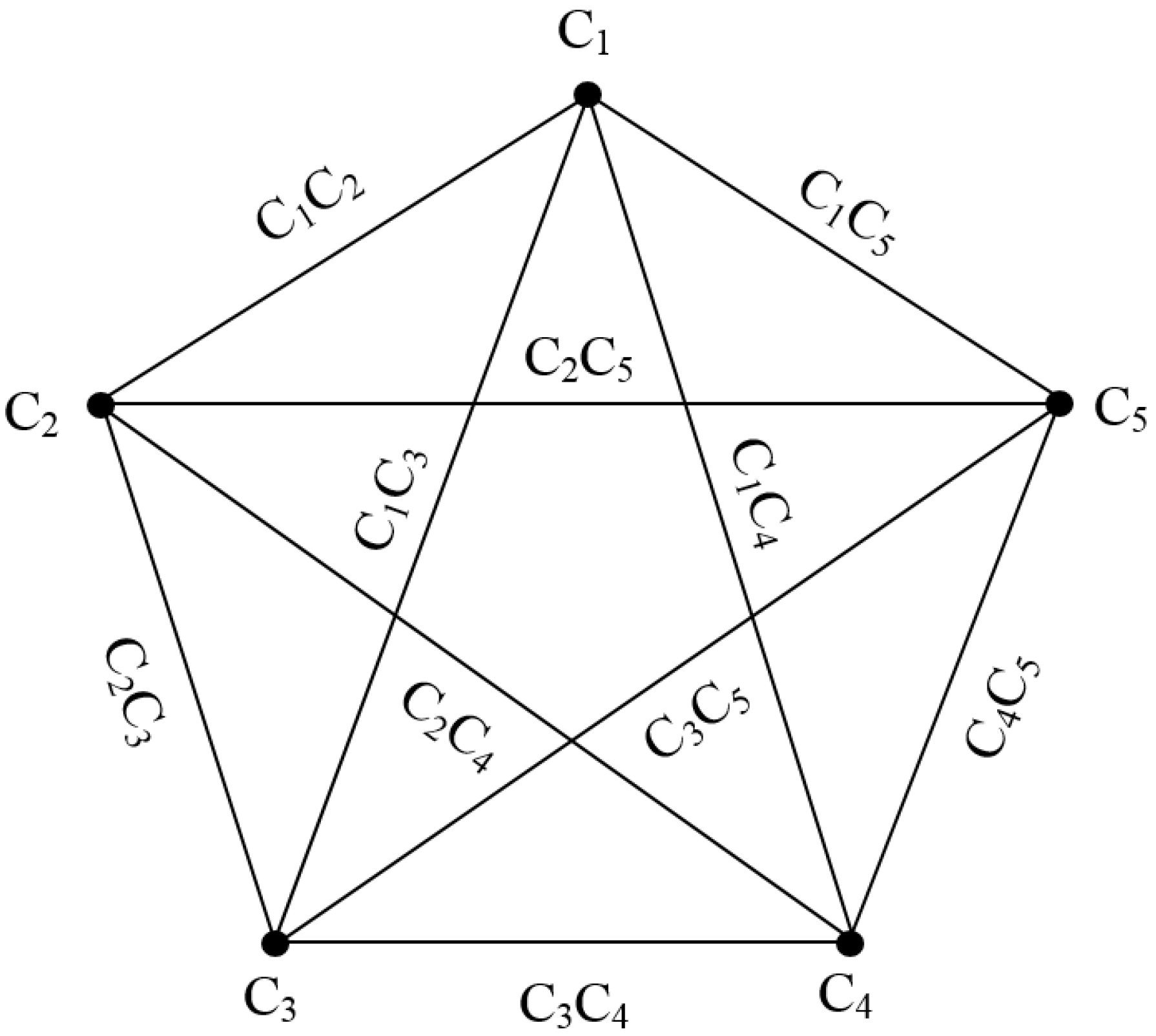
Suppose a team selected five places where they are interested in placing a tower, so that they can facilitate maximum numbers of the users. They observe the following two situations:

• Fixing a tower exactly at the chosen place from the selected five places
• Fixing a tower between any two of the selected five places.

For Situation $1,$ we proceed as follows:

Let $V=\{C_1,C_2,C_3,C_4,C_5\}$ be the set of places where the team is interested in fixing a tower as a vertex set. Suppose that $60\%$ of the experts on the team believe that $C_1$ should have a tower and $10\%$ of the experts believe that there is no need to fix tower at the place $C_1$ after carefully observing the different parameters. Thus, in this way, we can find the amplitude term for both membership and non-membership functions. Now, the phase term that represents the period needs to be found. Let $40\%$ of the experts believe that in a particular time $C_1$ can attract the maximum number of users (Profit) and $30\%$ of the experts have the opposite opinion. We model this information as $〈C_1:0.6e^{i0.4\pi },0.1e^{i0.3\pi }〉.$

Thus, the team finalizes its opinion about the place $C_1.$ Now, they visit the place $C_2$. After careful observation, they model the information as $〈C_2:0.7e^{i0.2\pi },0.2e^{i0.4\pi }〉$. It means that $70\%$ of the experts are in the favor of $C_2$, even though it will produce only $20\%$ of profit, while $20\%$ are opposed to $C_2$, even though it will produce $40\%$ profit. Similarly, they model all the other places as $〈C_3:0.5e^{i0.6\pi },0.7e^{i0.4\pi }〉,$ $〈C_4:0.7e^{i0.8\pi },0.5e^{i0.7\pi }〉$ and $〈C_5:0.4e^{i0.4\pi },0.9e^{i0.2\pi }〉.$ We denote this model as

$$A=\left\{\begin{array}{c}〈C_1:0.6e^{i0.4\pi },0.1e^{i0.3\pi }〉\\ 〈C_2:0.7e^{i0.2\pi },0.2e^{i0.4\pi }〉\\ 〈C_3:0.5e^{i0.6\pi },0.7e^{i0.4\pi }〉\\ 〈C_4:0.7e^{i0.8\pi },0.5e^{i0.7\pi }〉\\ 〈C_5:0.4e^{i0.4\pi },0.9e^{i0.2\pi }〉\end{array}\right.$$

The complex membership of the vertices denotes the positive characteristics and complex non-membership of the vertices denotes the negative characteristics of a certain parameter for a certain place. Now, finding the absolute values, we have

$$\begin{array}{cc}\hfill |C_1|& =(0.6,0.1),\hfill \\ \hfill |C_2|& =(0.7,0.2),\hfill \\ \hfill |C_3|& =(0.5,0.7),\hfill \\ \hfill |C_4|& =(0.7,0.5),\hfill \\ \hfill |C_5|& =(0.4,0.9).\hfill \end{array}$$

To find the optimal choice, we find the score function of the absolute values of $C_1,C_2,C_3,C_4,C_5.$ Thus, we have

$$\begin{array}{cc}\hfill S\left(C_1\right)& =0.6-0.1=0.5,\hfill \\ \hfill S\left(C_2\right)& =0.7-0.2=0.5,\hfill \\ \hfill S\left(C_3\right)& =0.5-0.7=-0.2,\hfill \\ \hfill S\left(C_4\right)& =0.7-0.5=0.2,\hfill \\ \hfill S\left(C_5\right)& =0.4-0.9=-0.5.\hfill \end{array}$$

Since the scores for $C_1$ and $C_2$ are equal, we find the accuracies of $C_1$ and $C_2:$ $H\left(C_1\right)=0.6+0.1=0.7$ and $H\left(C_2\right)=0.7+0.2=0.9,$ thus $C_1>C_2$, which is the most suitable choice to fix a tower. This is the application of complex intuitionistic fuzzy graph, where it has no edge, as shown in Figure 14.

Now, for Situation $2,$ we proceed as follows:

If a tower is fixed between places $C_1$ and $C_2$, it will represent the edge $C_1{C}_2$ of the vertex $C_1,C_2.$ To find the model of $C_1{C}_2$, we use Definition 6 and find that $〈C_1{C}_2:0.6e^{i0.4\pi },0.2e^{i0.4\pi }〉.$ Similarly, we find the other edges and we denote this model as

$$B=\left\{\begin{array}{c}〈C_1{C}_2:0.6e^{i0.4\pi },0.2e^{i0.4\pi }〉\\ 〈C_1{C}_3:0.5e^{i0.4\pi },0.7e^{i0.4\pi }〉\\ 〈C_1{C}_4:0.6e^{i0.4\pi },0.5e^{i0.7\pi }〉\\ 〈C_2{C}_4:0.7e^{i0.2\pi },0.5e^{i0.7\pi }〉\\ 〈C_1{C}_5:0.4e^{i0.4\pi },0.9e^{i0.3\pi }〉\\ 〈C_2{C}_3:0.5e^{i0.2\pi },0.7e^{i0.4\pi }〉\\ 〈C_2{C}_5:0.4e^{i0.2\pi },0.9e^{i0.4\pi }〉\\ 〈C_3{C}_4:0.5e^{i0.6\pi },0.7e^{i0.7\pi }〉\\ 〈C_3{C}_5:0.4e^{i0.4\pi },0.9e^{i0.4\pi }〉\\ 〈C_4{C}_5:0.4e^{i0.4\pi },0.9e^{i0.7\pi }〉\end{array}\right.$$

If we consider the edge $〈C_1{C}_2:0.6e^{i0.4\pi },0.2e^{i0.4\pi }〉$. In this case, the amplitude term shows that $60\%$ of the experts believe that there should be a tower between these two places and $20\%$ of the experts believe the opposite. The phase terms show that $40\%$ of the experts believe that in a certain time if a tower is fixed between these two places it will produce maximum profit, while $40\%$ of the experts believe the opposite. Absolute values of the edges are:

$$\begin{array}{cc}\hfill |C_1{C}_2|& =(0.6,0.2),|C_1{C}_3|=(0.5,0.7)\hfill \\ \hfill |C_1{C}_4|& =(0.6,0.5),|C_2{C}_4|=(0.7,0.5)\hfill \\ \hfill |C_1{C}_5|& =(0.4,0.9),|C_2{C}_3|=(0.5,0.7)\hfill \\ \hfill |C_2{C}_5|& =(0.4,0.9),|C_3{C}_4|=(0.5,0.9)\hfill \\ \hfill |C_3{C}_5|& =(0.4,0.9),|C_4{C}_5|=(0.4,0.9)\hfill \end{array}$$

To find the optimal choice, we find the score function of the absolute values of the edges. Thus, we have

$$\begin{array}{cc}\hfill S\left(C_1{C}_2\right)& =0.4,S\left(C_1{C}_3\right)=-0.2,\hfill \\ \hfill S\left(C_1{C}_4\right)& =0.1,S\left(C_2{C}_4\right)=0.2,\hfill \\ \hfill S\left(C_1{C}_5\right)& =-0.5,S\left(C_2{C}_3\right)=-0.2,\hfill \\ \hfill S\left(C_2{C}_5\right)& =-0.5,S\left(C_3{C}_4\right)=-0.4,\hfill \\ \hfill S\left(C_3{C}_5\right)& =-0.5,S\left(C_4{C}_5\right)=-0.5.\hfill \end{array}$$

$S\left(C_1{C}_2\right)=0.4$ is the greatest, and hence most suitable choice to fix the tower. This is the case where complex intuitionistic fuzzy graph has edges, as shown in Figure 15.

7. Conclusions

We defined cif-graphs and accomplished the notion of union of cif-graphs, Cartesian product of cif-graphs, join of cif-graphs and composition of cif-graphs. Our presented approach is the generalization of fuzzy graphs. We aim to extend our work in the following directions: One can see in the Section 6, that handling different parameters is one of the most difficult tasks, and since soft sets are very useful tools where one can handle more parameters in a practical way, we will define the complex fuzzy soft graphs that will generalize the idea of fuzzy graphs, soft graphs and fuzzy soft graphs. On the other side, since intuitionistic fuzzy sets generalize the concept of fuzzy sets, we will try to produce a model related with complex intuitionistic fuzzy soft graph, which is the generalization of complex fuzzy graphs and complex fuzzy soft graphs.

References

- Zadeh, L.A. Fuzzy sets. Inform. Control 1965, 8, 338–353. [Google Scholar] [CrossRef] [Green Version]
- Atanassov, K. Intuitionistic fuzzy sets. Fuzzy Sets Syst. 1986, 20, 87–96. [Google Scholar] [CrossRef]
- Palaniappan, N.; Srinivasan, R. Applications of intuitionistic fuzzy sets of root type in image processing. In Proceedings of the Annual Meeting of the North American Fuzzy Information Processing Society, Cincinnati, OH, USA, 14–17 June 2009; pp. 1–5. [Google Scholar]
- Szmidt, E.; Kacprzyk, J. An application of intuitionistic fuzzy set similarity measures to a multi-criteria decision making problem. In Proceedings of the Artificial Intelligence and Soft Computing—ICAISC, Zakopane, Poland, 25–29 June 2006; pp. 314–323. [Google Scholar]
- Vlachos, I.K.; Sergiadis, G.D. Intuitionistic fuzzy information: Applications to pattern recognition. Pattern Recognit. Lett. 2007, 28, 197–206. [Google Scholar] [CrossRef]
- Buckley, J.J. Fuzzy complex numbers. Fuzzy Sets Syst. 1989, 33, 333–345. [Google Scholar] [CrossRef]
- Nguyen, H.T.; Kandel, A.; Kreinovich, V. Complex fuzzy sets: Towards new foundations. In Proceedings of the Ninth IEEE International Conference on Fuzzy Systems, San Antonio, TX, USA, 7–10 May 2000; pp. 1045–1048. [Google Scholar]
- Ramot, D.; Milo, R.; Friedman, M.; Kandel, A. Complex fuzzy sets. IEEE Trans. Fuzzy Syst. 2002, 10, 171–186. [Google Scholar] [CrossRef]
- Ramot, D.; Friedman, M.; Langholz, G.; Kandel, A. Complex fuzzy logic. IEEE Trans. Fuzzy Syst. 2003, 11, 450–461. [Google Scholar] [CrossRef]
- Zhang, G.; Dillon, T.S.; Cai, K.Y.; Ma, J.; Lu, J. Operation properties and δ-equalities of complex fuzzy sets. Int. J. Approx. Reason. 2009, 50, 1227–1249. [Google Scholar] [CrossRef]
- Cheng, G.; Yang, J. Complex fuzzy reasoning schemes. In Proceedings of the IEEE International Conference on Information and Computing, Wuxi, China, 4–6 June 2010; pp. 29–32. [Google Scholar]
- Li, C.; Chan, F. Complex-fuzzy adaptive image restoration an artificial-bee-colony-based learning approach. In Proceedings of the Asian Conference on Intelligent Information and Database Systems, Daegu, Korea, 20–22 April 2011; pp. 90–99. [Google Scholar]
- Yager, R.R.; Abbasov, A.M. Pythagorean membership grades, complex numbers, and decision making. Int. J. Intell. Syst. 2013, 28, 436–452. [Google Scholar] [CrossRef]
- Alkouri, A.M.; Salleh, A.R. Complex intuitionistic fuzzy sets. AIP Conf. Proc. 2012, 1482, 464–470. [Google Scholar]
- Alkouri, A.M.; Salleh, A.R. Some operations on complex Atanassov’s intuitionistic fuzzy sets. AIP Conf. Proc. 2013, 1571, 987–993. [Google Scholar]
- Alkouri, A.M.; Salleh, A.R. Complex Atanassov’s intuitionistic fuzzy relation. Abstr. Appl. Anal. 2013, 2013, 287382. [Google Scholar] [CrossRef]
- Ali, M.; Tamir, D.E.; Rishe, N.D.; Kandel, A. Complex intuitionistic fuzzy classes. In Proceedings of the IEEE International Conference on Fuzzy Systems, Vancouver, BC, Canada, 24–29 July 2016; pp. 2027–2034. [Google Scholar]
- Rosenfeld, A. Fuzzy Graphs, Fuzzy Sets and Their Applications; Academic Press: New York, NY, USA, 1975; pp. 77–95. [Google Scholar]
- Mordeson, J.N.; Nair, P.S. Fuzzy Graphs and Fuzzy Hypergraphs, 2nd ed.; Physica Verlag: Heidelberg, Germany, 2001. [Google Scholar]
- Bhattacharya, P. Some remarks on fuzzy graphs. Pattern Recognit. Lett. 1987, 6, 297–302. [Google Scholar] [CrossRef]
- Thirunavukarasu, P.; Suresh, R.; Viswanathan, K.K. Energy of a complex fuzzy graph. Int. J. Math. Sci. Eng. Appl. 2016, 10, 243–248. [Google Scholar]
- Shannon, A.; Atanassov, A. A first step to a theory of the intuitionistic fuzzy graphs. In Proceedings of the First Workshop on Fuzzy Based Expert Systems, Sofia, Bulgaria, 28–30 September 1994; pp. 59–61. [Google Scholar]
- Akram, M.; Davvaz, B. Strong intuitionistic fuzzy graphs. Filomat 2012, 26, 177–196. [Google Scholar] [CrossRef]
- Akram, M.; Akmal, R. Operations on intuitionistic fuzzy graph structures. Fuzzy Inf. Eng. 2016, 8, 389–410. [Google Scholar] [CrossRef]
- Alshehri, N.; Akram, M. Intuitionistic fuzzy planar graphs. Discret. Dyn. Nat. Soc. 2014, 2014, 397823. [Google Scholar] [CrossRef]
- Karunambigai, M.G.; Akram, M.; Buvaneswari, R. Strong and superstrong vertices in intuitionistic fuzzy graphs. J. Intell. Fuzzy Syst. 2016, 30, 671–678. [Google Scholar] [CrossRef]
- Myithili, K.K.; Parvathi, R.; Akram, M. Certain types of intuitionistic fuzzy directed hypergraphs. Int. J. Mach. Learn. Cybern. 2016, 7, 287–295. [Google Scholar] [CrossRef]
- Nagoorgani, A.; Akram, M.; Anupriya, S. Double domination on intuitionistic fuzzy graphs. J. Appl. Math. Comput. 2016, 52, 515–528. [Google Scholar] [CrossRef]
- Parvathi, R.; Karunambigai, M.G.; Atanassov, K. Operations on intuitionistic fuzzy graphs. In Proceedings of the IEEE International Conference on Fuzzy Systems, Jeju Island, Korea, 20–24 August 2009; pp. 1396–1401. [Google Scholar]
- Parvathi, R.; Thamizhendhi, G. Domination in intuitionistic fuzzy graphs. Notes Intuit. Fuzzy Sets 2010, 12, 39–49. [Google Scholar]
- Dymova, L.; Sevastjanov, P.; Tikhonenko, A. A new approach to comparing intuitionistic fuzzy values. Sci. Res. Inst. Math. Comput. Sci. 2011, 10, 57–64. [Google Scholar]
- Liu, X.; Kim, H.S.; Feng, F.; Alcantud, J.C.R. Centroid Transformations of Intuitionistic Fuzzy Values Based on Aggregation Operators. Mathematics 2018, 6, 215. [Google Scholar] [CrossRef]
- Rashid, S.; Yaqoob, N.; Akram, M.; Gulistan, M. Cubic graphs with application. Int. J. Anal. Appl. 2018, 16, 733–750. [Google Scholar]
- Gulistan, M.; Khan, A.; Abdullah, A.; Yaqoob, N. Complex neutrosophic subsemigroups and ideals. Int. J. Anal. Appl. 2018, 16, 97–116. [Google Scholar]
- Gulistan, M.; Yaqoob, N.; Rashid, Z.; Smarandache, F.; Wahab, H.A. A study on neutrosophic cubic graphs with real life applications in industries. Symmetry 2018, 10, 203. [Google Scholar] [CrossRef]
Figure 1.
Complex intuitionistic fuzzy graph .
Figure 2.
Figure 3.
Figure 4.
Complex intuitionistic fuzzy graph of .
Figure 5.
Complex intuitionistic fuzzy graphs of and .
Figure 6.
Figure 7.
Figure 8.
Figure 9.
Figure 10.
Figure 11.
Figure 12.
Figure 13.
Figure 14.
Complex intuitionistic fuzzy graph with no edge.
Figure 15.
Complex intuitionistic fuzzy graph with edges.
© 2019 by the authors. Licensee MDPI, Basel, Switzerland. This article is an open access article distributed under the terms and conditions of the Creative Commons Attribution (CC BY) license (http://creativecommons.org/licenses/by/4.0/).
Share and Cite
MDPI and ACS Style
Yaqoob, N.; Gulistan, M.; Kadry, S.; Wahab, H.A. Complex Intuitionistic Fuzzy Graphs with Application in Cellular Network Provider Companies. Mathematics 2019, 7, 35. https://doi.org/10.3390/math7010035
AMA Style
Yaqoob N, Gulistan M, Kadry S, Wahab HA. Complex Intuitionistic Fuzzy Graphs with Application in Cellular Network Provider Companies. Mathematics. 2019; 7(1):35. https://doi.org/10.3390/math7010035
Chicago/Turabian StyleYaqoob, Naveed, Muhammad Gulistan, Seifedine Kadry, and Hafiz Abdul Wahab. 2019. "Complex Intuitionistic Fuzzy Graphs with Application in Cellular Network Provider Companies" Mathematics 7, no. 1: 35. https://doi.org/10.3390/math7010035
Note that from the first issue of 2016, this journal uses article numbers instead of page numbers. See further details here.