NC-Cross Entropy Based MADM Strategy in Neutrosophic Cubic Set Environment

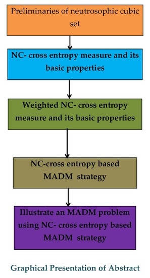
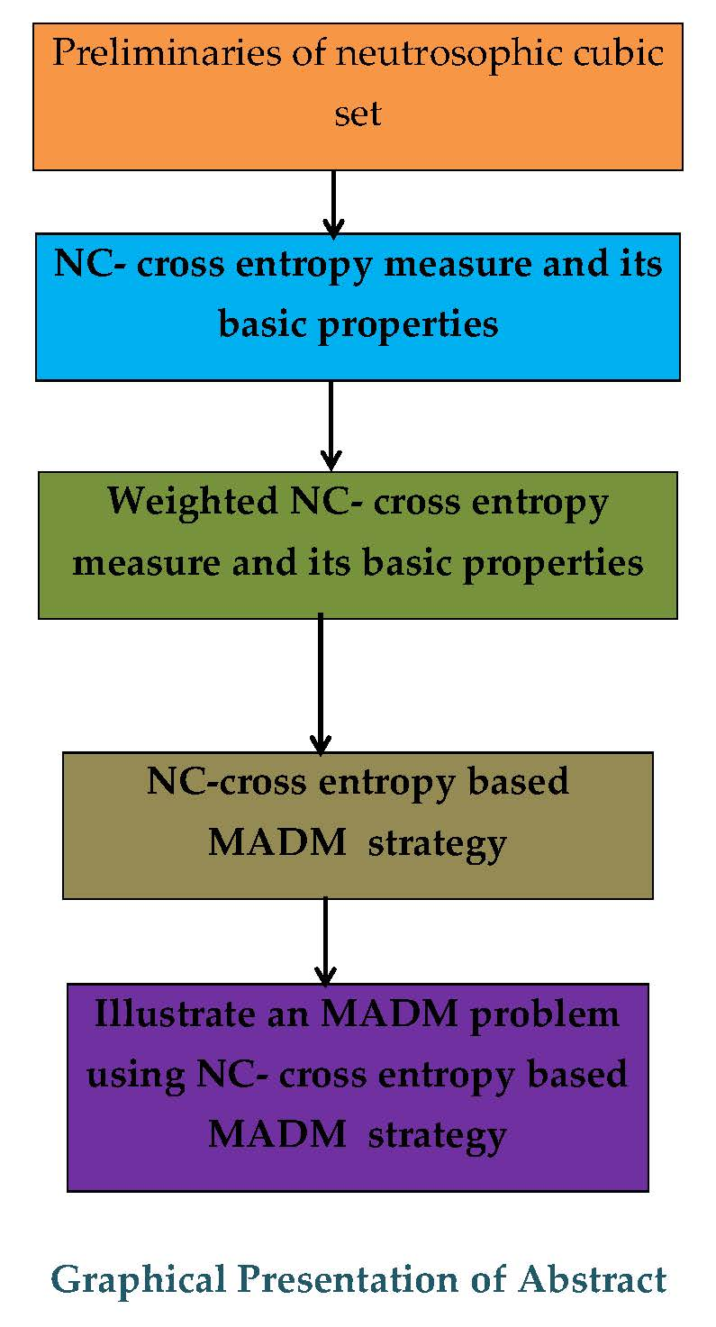
Abstract

The objective of the paper is to introduce a new cross entropy measure in a neutrosophic cubic set (NCS) environment, which we call NC-cross entropy measure. We prove its basic properties. We also propose weighted NC-cross entropy and investigate its basic properties. We develop a novel multi attribute decision-making (MADM) strategy based on a weighted NC-cross entropy measure. To show the feasibility and applicability of the proposed multi attribute decision-making strategy, we solve an illustrative example of the multi attribute decision-making problem.

1. Introduction

In 1998, Smarandache [1] introduced the neutrosophic set by considering membership (truth), indeterminacy, non-membership (falsity) functions as independent components to uncertain, inconsistent and incomplete information. In 2010, Wang et al. [2] defined the single valued neutrosophic set (SVNS), a subclass of neutrosophic sets to deal with real and scientific and engineering applications. In the medical domain, Ansari et al. [3] employed the neutrosophic set and neutrosophic inference to knowledge based systems. Several researchers applied neutrosophic sets effectively for image segmentation problems [4,5,6,7,8,9]. Neutrosophic sets are also applied for integrating geographic information system data [10] and for binary classification problems [11].

Pramanik and Chackrabarti [12] studied the problems faced by construction workers in West Bengal in order to find its solutions using neutrosophic cognitive maps [13]. Based on the experts’ opinion and the notion of indeterminacy, the authors formulated a neutrosophic cognitive map and studied the effect of two instantaneous state vectors separately on a connection matrix and neutrosophic adjacency matrix. Mondal and Pramanik [14] identified some of the problems of Hijras (third gender), namely, absence of social security, education problems, bad habits, health problems, stigma and discrimination, access to information and service problems, violence, issues of the Hijra community, and sexual behavior problems. Based on the experts’ opinion and the notion of indeterminacy, the authors formulated a neutrosophic cognitive map and presented the effect of two instantaneous state vectors separately on a connection matrix and neutrosophic adjacency matrix.

Pramanik and Roy [15] studied the game theoretic model [16] of the Jammu and Kashmir conflict between India and Pakistan in a SVNS environment. The authors examined the progress and the status of the conflict, as well as the dynamics of the relationship by focusing on the influence of United States of America, India and China in crisis dynamics. The authors investigated the possible solutions. The authors also explored the possibilities and developed arguments for an application of the principle of neutrosophic game theory to present a standard 2 × 2 zero-sum game theoretic model to identify an optimal solution.

Maria Sodenkamp applied the concept of SVNSs in multi attribute decision-making (MADM) in her Ph. D. thesis [17] in 2013. In 2018, Pranab Biswas [18] studied various strategies for MADM in SVNS environment in his Ph. D. thesis. Kharal [19] presented an MADM strategy in a single valued neutrosophic environment and presented the application of the proposed strategy for the evaluation of university professors for tenure and promotions. Mondal and Pramanik [20] extended the teacher selection strategy [21] in SVNS environments. Mondal and Pramanik [22] also presented MADM strategy to school choice problems in SVNS environments. Mondal and Pramanik [23] presented an MADM decision-making model for clay-brick selection in a construction field based on grey relational analysis in SVNS environments. Biswas et al. [24,25,26] presented several MADM strategies in single valued neutrosophic environments such as technique for order of preference by similarity to ideal solution (TOPSIS) [24], grey relational analysis [25], and entropy based MADM [26]. Several studies [27,28,29,30], using similarity measures based MADM, have been proposed in SVNS environments. Several studies enrich the study of MADM in SVNS environments such as projection and bidirectional projection measure based MADM [31], maximizing deviation method [32], Frank prioritized Bonferroni mean operator based MADM [33], biparametric distance measures based MADM [34], prospect theory based MADM [35], multi-objective optimization by ratio analysis plus the full multiplicative form (MULTIMOORA) [36], weighted aggregated sum product assessment (WASPAS) [37,38], complex proportional assessment (COPRAS) [39], TODIM [40], projection based TODIM [41], outranking [42], analytic hierarchy process (AHP) [43], and VIsekriterijumska optimizacija i KOmpromisno Resenje (VIKOR) [44].

In 2005, Wang et al. [45] introduced the interval neutrosophic set (INS) by considering membership function, non-membership function and indeterminacy function as independent functions that assume the values in interval form. Pramanik and Mondal [46] extended the single valued neutrosophic grey relational analysis method to interval neutrosophic environments and applied it to an MADM problem. The authors employed an information entropy method, which is used to obtain the unknown attribute weights and presented a numerical example. Dey et al. [47] investigated an extended grey relational analysis strategy for MADM problems in uncertain interval neutrosophic linguistic environments. The authors solved a numerical example and compared the obtained results with results obtained from the other existing strategies in the literature. Dey et al. [48] developed two MADM strategies in INS environment based on the combination of angle cosine and projection method. The authors presented an illustrative numerical example in the Khadi institution to demonstrate the effectiveness of the proposed MADM strategies. Several studies enrich the development of MADM in INS environments such as VIKOR [49], TOPSIS [50,51], outranking strategy [52], similarity measure [29,53,54,55], weighted correlation coefficient based MADM strategy [56], and generalized weighted aggregation operator based MADM strategy [57]. The study in recent trends in neutrosophic theory and applications can be found in [58].

Ali et al. [59] proposed the neutrosophic cubic set (NCS) by hybridizing NS and INS. Banerjee et al. [60] developed the grey relational analysis based MADM strategy in NCS environments. Pramanik et al. [61] presented an Extended TOPSIS strategy for MADM in NCS environments with neutrosophic cubic information. Zhan et al. [62] developed an MADM strategy based on two weighted average operators in NCS environments. Lu and Ye [63] presented three cosine measures between NCSs and established three MADM strategies in NCS environments. Shi and Ye [64] introduced Dombi aggregation operators of NCSs and applied for an MADM problem. Ye [65] presented operations and an aggregation method of neutrosophic cubic numbers for MADM. For multi attribute group decision-making (MAGDM), Pramanik et al. [66] defined a similarity measure for NCSs and proved some of its basic properties and developed a new MAGDM strategy with linguistic variables in NCS environments. To develop TODIM, Pramanik et al. [67] proposed the score and accuracy functions for NCSs and proved their basic properties, and developed a strategy for ranking of neutrosophic cubic numbers based on the score and accuracy functions. In the same study, Pramanik et al. [67] presented a numerical example and presented a comparison analysis. In the same study, Pramanik et al. [67] conducted a sensitivity analysis to reflect the impact of ranking order of the alternatives for different values of attenuation factor of losses for MAGDM strategies.

Pramanik et al. [68] proposed a new VIKOR strategy for MAGDM in NCS environments. The authors also presented sensitivity analysis to reflect the impact of different values of the decision-making mechanism coefficient on ranking order of the alternatives.

Cross entropy measure is an important measure to calculate the divergence of any variable from prior one variable. In 1968, Zadeh [69] first proposed fuzzy entropy to deal with the divergence of two fuzzy variables. Thereafter, Deluca and Termini [70] introduced some axioms of fuzzy entropy involving Shannon’s function [71]. Szmidt and Kacprzyk [72] proposed an entropy measure for intuitionistic fuzzy sets (IFSs) by employing a geometric interpretation of IFS. Majumder and Samanta [73] introduced a SVNS based entropy measure and similarity measure. Furthermore, Aydogdu [74] proposed an entropy measure for INSs. Ye and Du [75] proposed some entropy measures for INS based on the distances as the extension of the entropy measures of interval valued IFS. Shang and Jiang [76] defined cross entropy in a fuzzy environment between two fuzzy variables. Vlachos and Sergiadis [77] defined intuitionistic fuzzy cross-entropy. Ye [78] employed intuitionistic fuzzy cross entropy to multi criteria decision-making (MCDM). Maheshwari and Srivastava [79] proposed new cross entropy in intuitionistic fuzzy environment and employed it to medical diagnosis. Zhang et al. [80] defined entropy and cross entropy measure for interval-intuitionistic sets and discuss their properties. Ye [81] proposed an interval intuitionistic fuzzy cross entropy measure and employed it to solve MCDM problems.

Ye [82] defined cross entropy for SVNSs and employed it solve to MCDM problems. To remove the drawbacks of cross entropy [82], Ye [83] proposed another cross entropy for SVNSs. In the same study, Ye [83] also proposed new cross entropy for INSs. Tian et al. [84] proposed a cross entropy for INS environments and employed it to MCDM problems. Sahin [85] proposed an interval neutrosophic cross entropy measure based on fuzzy cross entropy and single valued neutrosophic cross entropy measures and applied it to MCDM problems. Recently, Pramanik et al. [86] proposed a novel cross entropy, namely, NS-cross entropy in SVNS environments and proved its basic properties. In the same research, Pramanik et al. [86] also proposed weighted NS-cross entropy and employed it to MAGDM problem. Furthermore, Dalapati et al. [87] extended NS-cross entropy in INS environments and employed it for solving MADM problems. Pramanik et al. [88] developed two new MADM strategies based on cross entropy measures in bipolar neutrosophic set (BNS) and interval BNS environments.

1.1. Research Gap: NC-Cross Entropy-Based MADM Strategy in NCS Environments

This study answers the following research questions:

• Is it possible to introduce an NC-cross entropy measure in NCS environments?
• Is it possible to introduce a weighted cross entropy measure in NCS environments?
• Is it possible to develop a novel MADM strategy based on weighted NC-cross entropy?

1.2. Motivation

The studies [59,60,61,62,63,64,65,66,67,68] reveal that cross entropy measure is not proposed in NCS environments. Since MADM strategy is not studied in the literature, we move to propose a comprehensive NC-cross entropy-based strategy for tackling MADM in the NCS environments. This study develops a novel NC-cross entropy-based MADM strategy.

The objectives of the paper are:

• To introduce a NC-cross entropy measure and establish its basic properties in an NCS environment.
• To introduce a weighted NC- cross measure and establish its basic properties in NCS environments.
• To develop a novel MADM strategy based on weighted NC-cross entropy measure in NCS environments.

To fill the research gap, we propose NC-cross entropy-based MADM strategy.

The remainder of the paper is presented as follows: In Section 2, we describe the basic definitions and operation of SVNSs, INSs, and NCSs. In Section 3, we propose an NC-cross entropy measure and a weighted NC-cross entropy measure and establish their basic properties. Section 4 is devoted to developing MADM strategy using NC-cross entropy. Section 5 provides an illustrative numerical example to show the applicability and validity of the proposed strategy in NCS environments. Section 6 presents briefly the contribution of the paper. Section 7 offers conclusions and the future scope of research.

2. Preliminaries

In this section, some basic concepts and definitions of SVNS, INS and NCS are presented that will be utilized to develop the paper.

Definition 1.

Single valued neutrosophic set (SVNS)

Assume that U is a space of points (objects) with a generic element u $\in$ U. A SVNS [2] H in U is characterized by a truth-membership function ${\mathrm{T}}_{\mathrm{H}}(\mathrm{u}),$ an indeterminacy-membership function ${\mathrm{I}}_{\mathrm{H}}(\mathrm{u}),$ and a falsity-membership function ${\mathrm{F}}_{\mathrm{H}}(\mathrm{u}),$ where ${\mathrm{T}}_{\mathrm{H}}(\mathrm{u}),$ ${\mathrm{I}}_{\mathrm{H}}(\mathrm{u}),$ ${\mathrm{F}}_{\mathrm{H}}(\mathrm{u})\in [0, 1]$ for each point u in U. Therefore, a SVNS A is expressed as

$$\mathrm{H}=\{\mathrm{u}, {\mathrm{T}}_{\mathrm{H}}(\mathrm{u}), {\mathrm{I}}_{\mathrm{H}}(\mathrm{u}), {\mathrm{F}}_{\mathrm{H}}(\mathrm{u})|\mathrm{u}\in \mathrm{U}\},$$

(1)

whereas the sum of ${\mathrm{T}}_{\mathrm{H}}(\mathrm{u}),$ ${\mathrm{I}}_{\mathrm{H}}(\mathrm{u})$ and ${\mathrm{F}}_{\mathrm{H}}(\mathrm{u})$ satisfies the condition:

$${0\le \mathrm{T}}_{\mathrm{H}}(\mathrm{u})+{\mathrm{I}}_{\mathrm{H}}(\mathrm{u})+{\mathrm{F}}_{\mathrm{H}}(\mathrm{u})\le 3.$$

(2)

The order triplet $<\mathrm{T}, \mathrm{I}, \mathrm{F}>$ is called a single valued neutrosophic number (SVNN).

Example 1.

Let H be any SVNS in U; then, H can be expressed as: $\mathrm{H}=\{\mathrm{u}, (0.7, 0.3, 0.5)| \mathrm{u}\in \mathrm{U}\}$ and SVNN presented as: $\mathrm{H}= <0.7, 0.3, 0.5)>$.

Definition 2.

Inclusion of SVNS

The inclusion of any two SVNSs [2] ${\mathrm{H}}_1$ and ${\mathrm{H}}_2$ in U is denoted by ${\mathrm{H}}_1\subseteq {\mathrm{H}}_2$ and defined as follows:

$${\mathrm{H}}_1\subseteq {\mathrm{H}}_2 iff {\mathrm{T}}_{{\mathrm{H}}_1}(\mathrm{u})\le {\mathrm{T}}_{{\mathrm{H}}_2}(\mathrm{u}), {\mathrm{I}}_{{\mathrm{H}}_1}(\mathrm{u})\ge {\mathrm{I}}_{{\mathrm{H}}_2}(\mathrm{u}), {\mathrm{F}}_{{\mathrm{H}}_1}(\mathrm{u})\ge {\mathrm{F}}_{{\mathrm{H}}_2}(\mathrm{u}) \mathit{for} \mathit{all} \mathrm{u}\in \mathrm{U}.$$

(3)

Example 2.

Let ${\mathrm{H}}_1$ and ${\mathrm{H}}_2$ be any two SVNNs in U presented as follows: ${\mathrm{H}}_1= <(0.7, 0.3, 0.5)>$ and ${\mathrm{H}}_2= <(0.8, 0.2, 0.4)>$ for all $\mathrm{u}\in \mathrm{U}.$ Using the property of inclusion of two SVNNs, we conclude that ${\mathrm{H}}_1\subseteq {\mathrm{H}}_2.$

Definition 3.

Equality of two SVNS

The equality of any two SVNSs [2] H₁ and H₂ in U denoted by ${\mathrm{H}}_1={\mathrm{H}}_2$ is defined as:

$${\mathrm{T}}_{{\mathrm{H}}_1}(\mathrm{u})={\mathrm{T}}_{{\mathrm{H}}_2}(\mathrm{u}), {\mathrm{I}}_{{\mathrm{H}}_1}(\mathrm{u})={\mathrm{I}}_{{\mathrm{H}}_2}(\mathrm{u}) \mathit{and} {\mathrm{F}}_{{\mathrm{H}}_1}(\mathrm{u})={\mathrm{F}}_{{\mathrm{H}}_2}(\mathrm{u}) \mathit{for} \mathit{all} \mathrm{u}\in \mathrm{U}.$$

(4)

Definition 4.

Complement of any SVNS

The complement of any SVNS [2] H in U denoted by ${\mathrm{H}}^{\mathrm{c}}$ and defined as follows:

$${\mathrm{H}}^{\mathrm{c}}=\{\mathrm{u}, 1-{\mathrm{T}}_{\mathrm{H}},1-{\mathrm{I}}_{\mathrm{H}}, 1-{\mathrm{F}}_{\mathrm{H}} |\mathrm{u}\in \mathrm{U}\text{}}.$$

(5)

Example 3.

Let H be any SVNN in U presented as follows:

$\mathrm{H}= <0.7, 0.3, 0.5)>$. Then, the compliment of H is obtained as ${\mathrm{H}}^{\mathrm{c}}= <(0.3, 0.7, 0.5)>$.

Definition 5.

Union of two SVNSs

The union of two SVNSs [2] ${\mathrm{H}}_1$ and ${\mathrm{H}}_2$ is a neutrosophic set ${\mathrm{H}}_3$ (say) written as ${\mathrm{H}}_3={\mathrm{H}}_1 \cup {\mathrm{H}}_2.$

Here,

$$\begin{gathered} {\mathrm{T}}_{{\mathrm{H}}_3}(\mathrm{u})=\max \{{\mathrm{T}}_{{\mathrm{H}}_1}(\mathrm{u}), {\mathrm{T}}_{{\mathrm{H}}_2}(\mathrm{u})\}, {\mathrm{I}}_{{\mathrm{H}}_3}(\mathrm{u})=\min \{{\mathrm{I}}_{{\mathrm{H}}_1}(\mathrm{u}), {\mathrm{I}}_{{\mathrm{H}}_2}(\mathrm{u})\}, \\ {\mathrm{F}}_{{\mathrm{H}}_3}(\mathrm{u})=\min \{{\mathrm{F}}_{{\mathrm{H}}_1}(\mathrm{u}), {\mathrm{F}}_{{\mathrm{H}}_2}(\mathrm{u})\}, \forall \mathrm{u}\in \mathrm{U}. \end{gathered}$$

(6)

Example 4.

Let ${\mathrm{H}}_1$ and ${\mathrm{H}}_2$ be two SVNNs in U presented as follows:

Let ${\mathrm{H}}_1= <(0.6, 0.3, 0.4)>$ and ${\mathrm{H}}_2= <(0.7, 0.3, 0.6)>$ be two SVNNs. Then union of them is obtained using Equation (6) as follows: ${\mathrm{H}}_1 \cup {\mathrm{H}}_2 = <(0.7, 0.3, 0.4)>.$

Definition 6.

Intersection of any two SVNSs

The intersection of two SVNSs [2] ${\mathrm{H}}_1$ and ${\mathrm{H}}_2$ denoted by ${\mathrm{H}}_4$ and defined as ${\mathrm{H}}_4={\mathrm{H}}_1\cap {\mathrm{H}}_2.$

Here,

$$\begin{gathered} {\mathrm{T}}_{{\mathrm{H}}_4}(\mathrm{u})=\min \{{\mathrm{T}}_{{\mathrm{H}}_1}(\mathrm{u}), {\mathrm{T}}_{{\mathrm{H}}_2}(\mathrm{u})\}, {\mathrm{I}}_{{\mathrm{H}}_4}(\mathrm{u})=\max \{{\mathrm{I}}_{{\mathrm{H}}_1}(\mathrm{u}), {\mathrm{I}}_{{\mathrm{H}}_2}(\mathrm{u})\}, \\ {\mathrm{F}}_{{\mathrm{H}}_4}(\mathrm{u})=\max \{{\mathrm{F}}_{{\mathrm{H}}_1}(\mathrm{u}), {\mathrm{F}}_{{\mathrm{H}}_2}(\mathrm{u})\}, \forall \mathrm{u}\in \mathrm{U}. \end{gathered}$$

(7)

Example 5.

Let ${\mathrm{H}}_1$ and ${\mathrm{H}}_2$ be two SVNNs in U presented as follows:

${\mathrm{H}}_1= <(0.6, 0.3, 0.4)> \mathrm{and} {\mathrm{H}}_2= <(0.7, 0.3, 0.6)>.$ Then, the intersection of them is obtained using Equation (7) as follows:

$${\mathrm{H}}_1\cap {\mathrm{H}}_2= <(0.6, 0.3, 0.6)>.$$

Definition 7.

Some operations of SVNS

Let ${\mathrm{H}}_1$ and ${\mathrm{H}}_2$ be any two SVNSs [2]. Then, addition and multiplication are defined as:

$${\mathrm{H}}_1 \oplus {\mathrm{H}}_2= <{\mathrm{T}}_{{\mathrm{H}}_1}(\mathrm{u})+{\mathrm{T}}_{{\mathrm{H}}_2}(\mathrm{u})-{\mathrm{T}}_{{\mathrm{H}}_1}(\mathrm{u}) .{\mathrm{T}}_{{\mathrm{H}}_2}(\mathrm{u}), {\mathrm{I}}_{{\mathrm{H}}_1}(\mathrm{u}) .{\mathrm{I}}_{{\mathrm{H}}_2}(\mathrm{u}), {\mathrm{F}}_{{\mathrm{H}}_1}(\mathrm{u}) . {\mathrm{F}}_{{\mathrm{H}}_2}(\mathrm{u}) >, \forall \mathrm{u}\in \mathrm{U}.$$

(8)

$${\mathrm{H}}_1\otimes {\mathrm{H}}_2= <{\mathrm{T}}_{{\mathrm{H}}_1}(\mathrm{u}) .{\mathrm{T}}_{{\mathrm{H}}_2}(\mathrm{u}),{\mathrm{I}}_{{\mathrm{H}}_1}(\mathrm{u})+{\mathrm{I}}_{{\mathrm{H}}_2}(\mathrm{u})-{\mathrm{I}}_{{\mathrm{H}}_1}(\mathrm{u}) .{\mathrm{I}}_{{\mathrm{H}}_2}(\mathrm{u}), {\mathrm{F}}_{{\mathrm{H}}_1}(\mathrm{u})+{\mathrm{F}}_{{\mathrm{H}}_2}(\mathrm{u})-{\mathrm{F}}_{{\mathrm{H}}_1}(\mathrm{u}) .{\mathrm{F}}_{{\mathrm{H}}_2}(\mathrm{u}) >, \forall \mathrm{u}\in \mathrm{U}.$$

(9)

Example 6.

Let ${\mathrm{H}}_1$ and ${\mathrm{H}}_2$ be two SVNSs in U presented as follows:

${\mathrm{H}}_1= <(0.6, 0.3, 0.4)> \mathrm{and} {\mathrm{H}}_2= <(0.7, 0.3, 0.6)> .$

Then, using Equations (8) and (9), we obtained ${\mathrm{H}}_1\oplus {\mathrm{H}}_2$ and ${\mathrm{H}}_1\otimes {\mathrm{H}}_2$ as follows:

1. 

${\mathrm{H}}_1\oplus {\mathrm{H}}_2= <(0.88, 0.09, 0.24)>.$

2. 

${\mathrm{H}}_1 \otimes {\mathrm{H}}_2= <(0.42, 0.51, 0.76)>.$

Definition 8.

Interval neutrosophic set (INS)

Assume that U is a space of points (objects) with a generic element $\mathrm{u}\in \mathrm{U}.$ An INS [45] J in U is characterized by a truth-membership function ${\mathrm{T}}_{\mathrm{J}}(\mathrm{u})$, an indeterminacy-membership function ${\mathrm{I}}_{\mathrm{J}}(\mathrm{u})$, and a falsity-membership function ${\mathrm{F}}_{\mathrm{J}}(\mathrm{u}),$ where ${\mathrm{T}}_{\mathrm{J}}(\mathrm{u})=[{\mathrm{T}}_{\mathrm{J}}^{-}(\mathrm{u}), {\mathrm{T}}_{\mathrm{J}}^{+}(\mathrm{u})]$, ${\mathrm{I}}_{\mathrm{J}}(\mathrm{u})=[{\mathrm{I}}_{\mathrm{J}}^{-}(\mathrm{u}), {\mathrm{I}}_{\mathrm{J}}^{+}(\mathrm{u})]$, ${\mathrm{F}}_{\mathrm{J}}(\mathrm{u})=[{\mathrm{F}}_{\mathrm{J}}^{-}(\mathrm{u}), {\mathrm{F}}_{\mathrm{J}}^{+}(\mathrm{u})]$ for each point u in U. Therefore, a INSs J can be expressed as

$$\mathrm{J}=\{\mathrm{u}, [{\mathrm{T}}_{\mathrm{J}}^{-}(\mathrm{u}), {\mathrm{T}}_{\mathrm{J}}^{+}(\mathrm{u})], [{\mathrm{I}}_{\mathrm{J}}^{-}(\mathrm{u}), {\mathrm{I}}_{\mathrm{J}}^{+}(\mathrm{u})], [{\mathrm{F}}_{\mathrm{J}}^{-}(\mathrm{u}), {\mathrm{F}}_{\mathrm{J}}^{+}(\mathrm{u})] |\mathrm{u}\in \mathrm{U}\},$$

(10)

where ${\mathrm{T}}_{\mathrm{J}}^{-}(\mathrm{u}), {\mathrm{T}}_{\mathrm{J}}^{+}(\mathrm{u})$, ${\mathrm{I}}_{\mathrm{J}}^{-}(\mathrm{u}), {\mathrm{I}}_{\mathrm{J}}^{+}(\mathrm{u})$, ${\mathrm{F}}_{\mathrm{J}}^{-}(\mathrm{u}), {\mathrm{F}}_{\mathrm{J}}^{+}(\mathrm{u}) \subseteq [0, 1]$.

Definition 9.

Inclusion of two INSs

$$\begin{gathered} \mathit{Let} {\mathrm{J}}_1=\{\mathrm{u}, [{\mathrm{T}}_{{\mathrm{J}}_1}^{-}(\mathrm{u}), {\mathrm{T}}_{{\mathrm{J}}_1}^{+}(\mathrm{u})], [{\mathrm{I}}_{{\mathrm{J}}_1}^{-}(\mathrm{u}), {\mathrm{I}}_{{\mathrm{J}}_1}^{+}(\mathrm{u})], [{\mathrm{F}}_{{\mathrm{J}}_1}^{-}(\mathrm{u}), {\mathrm{F}}_{{\mathrm{J}}_1}^{+}(\mathrm{u})] |\mathrm{u}\in \mathrm{u}\} \mathit{and} \\ {\mathrm{J}}_2=\{\mathrm{u}, [{\mathrm{T}}_{{\mathrm{J}}_2}^{-}(\mathrm{u}), {\mathrm{T}}_{{\mathrm{J}}_2}^{+}(\mathrm{u})], [{\mathrm{I}}_{{\mathrm{J}}_2}^{-}(\mathrm{u}), {\mathrm{I}}_{{\mathrm{J}}_2}^{+}(\mathrm{u})], [{\mathrm{F}}_{{\mathrm{J}}_2}^{-}(\mathrm{u}), {\mathrm{F}}_{{\mathrm{J}}_2}^{+}(\mathrm{u})] |\mathrm{u}\in \mathrm{u}\} \mathit{be} \mathit{any} \mathit{two} \mathit{INSs} \mathit{[}\mathit{45}\mathit{]} \\ \mathit{in} \mathrm{u}, \mathit{then} {\mathrm{J}}_1\subseteq {\mathrm{J}}_2 \mathit{iff} {\mathrm{T}}_{{\mathrm{J}}_1}^{-}(\mathrm{u})\le {\mathrm{T}}_{{\mathrm{J}}_2}^{-}(\mathrm{u}),{\mathrm{T}}_{{\mathrm{J}}_1}^{+}(\mathrm{u})\le {\mathrm{T}}_{{\mathrm{J}}_2}^{+}(\mathrm{u}), {\mathrm{I}}_{{\mathrm{J}}_1}^{-}(\mathrm{u})\ge {\mathrm{I}}_{{\mathrm{J}}_2}^{-}(\mathrm{u}), {\mathrm{I}}_{{\mathrm{J}}_1}^{+}(\mathrm{u})\ge {\mathrm{I}}_{{\mathrm{J}}_2}^{+}(\mathrm{u}), \\ {\mathrm{F}}_{{\mathrm{J}}_1}^{-}(\mathrm{u})\ge {\mathrm{F}}_{{\mathrm{J}}_2}^{-}(\mathrm{u}), {\mathrm{F}}_{{\mathrm{J}}_1}^{+}(\mathrm{u}) \ge {\mathrm{F}}_{{\mathrm{J}}_2}^{+}(\mathrm{u}) \mathit{for} \mathit{all} \mathrm{u}\in \mathrm{u}. \end{gathered}$$

(11)

Definition 10.

Complement of an INS

The complement ${\mathrm{J}}^{\mathrm{c}}$ of an INS [45] $\mathrm{J}=\{ \mathrm{u}, [{\mathrm{T}}_{\mathrm{J}}^{-}(\mathrm{u}), {\mathrm{T}}_{\mathrm{J}}^{+}(\mathrm{u})], [{\mathrm{I}}_{\mathrm{J}}^{-}(\mathrm{u}), {\mathrm{I}}_{\mathrm{J}}^{+}(\mathrm{u})], [{\mathrm{F}}_{\mathrm{J}}^{-}(\mathrm{u}), {\mathrm{F}}_{\mathrm{J}}^{+}(\mathrm{u})] |\mathrm{u}\in \mathrm{U}\}$ is defined as follows:

$${\mathrm{J}}^{\mathrm{c}}=\{ \mathrm{u}, [{{1-\mathrm{T}}_{\mathrm{J}}^{+}(\mathrm{u}), 1-\mathrm{T}}_{\mathrm{J}}^{-}(\mathrm{u})], [{1-\mathrm{I}}_{\mathrm{J}}^{+}(\mathrm{u}), {1-\mathrm{I}}_{\mathrm{J}}^{-}(\mathrm{u})], [{1-\mathrm{F}}_{\mathrm{J}}^{+}(\mathrm{u}), 1-{\mathrm{F}}_{\mathrm{J}}^{-}(\mathrm{u})] |\mathrm{u}\in \mathrm{U}\}.$$

(12)

Definition 11.

Equality of two INSs

$$\begin{gathered} \mathit{Let} {\mathrm{J}}_1=\{\mathrm{u}, [{\mathrm{T}}_{{\mathrm{J}}_1}^{-}(\mathrm{u}), {\mathrm{T}}_{{\mathrm{J}}_1}^{+}(\mathrm{u})], [{\mathrm{I}}_{{\mathrm{J}}_1}^{-}(\mathrm{u}), {\mathrm{I}}_{{\mathrm{J}}_1}^{+}(\mathrm{u})], [{\mathrm{F}}_{{\mathrm{J}}_1}^{-}(\mathrm{u}), {\mathrm{F}}_{{\mathrm{J}}_1}^{+}(\mathrm{u})] |\mathrm{u}\in \mathrm{u}\} \mathit{and} \\ {\mathrm{J}}_2=\{\mathrm{u}, [{\mathrm{T}}_{{\mathrm{J}}_2}^{-}(\mathrm{u}), {\mathrm{T}}_{{\mathrm{J}}_2}^{+}(\mathrm{u})], [{\mathrm{I}}_{{\mathrm{J}}_2}^{-}(\mathrm{u}), {\mathrm{I}}_{{\mathrm{J}}_2}^{+}(\mathrm{u})], [{\mathrm{F}}_{{\mathrm{J}}_2}^{-}(\mathrm{u}), {\mathrm{F}}_{{\mathrm{J}}_2}^{+}(\mathrm{u})] |\mathrm{u}\in \mathrm{u}\} \mathit{be} \mathit{any} \mathit{two} \mathit{INSs} [\mathit{45}] \\ \mathit{in} \mathit{U}, \mathit{then} {\mathrm{J}}_1={\mathrm{J}}_2 \mathrm{iff} {\mathrm{T}}_{{\mathrm{J}}_1}^{-}(\mathrm{u})={\mathrm{T}}_{{\mathrm{J}}_2}^{-}(\mathrm{u}), {\mathrm{T}}_{{\mathrm{J}}_1}^{+}(\mathrm{u})={\mathrm{T}}_{{\mathrm{J}}_2}^{+}(\mathrm{u}), {\mathrm{I}}_{{\mathrm{J}}_1}^{-}(\mathrm{u})={\mathrm{I}}_{{\mathrm{J}}_2}^{-}(\mathrm{u}), \\ {\mathrm{I}}_{{\mathrm{J}}_1}^{+}(\mathrm{u})={\mathrm{I}}_{{\mathrm{J}}_2}^{+}(\mathrm{u}), {\mathrm{F}}_{{\mathrm{J}}_1}^{-}(\mathrm{u})={\mathrm{F}}_{{\mathrm{J}}_2}^{-}(\mathrm{u}), {\mathrm{F}}_{{\mathrm{J}}_1}^{+}(\mathrm{u})={\mathrm{F}}_{{\mathrm{J}}_2}^{+}(\mathrm{u}) \mathit{for} \mathit{all} \mathrm{u}\in \mathrm{U}. \end{gathered}$$

(13)

Definition 12.

Neutrosophic cubic set (NCS)

Assume that U is a space of points (objects) with a generic element ${\mathrm{u}}_{\mathrm{i}}\in \mathrm{U}.$ A NCS [59] Q in U is a hybrid structure of INS and SVNS that can be expressed as follows:

$$\mathrm{Q}=\{{\mathrm{u}}_{\mathrm{i}}, <[{\mathrm{T}}_{\mathrm{Q}}^{-}({\mathrm{u}}_{\mathrm{i}}), {\mathrm{T}}_{\mathrm{Q}}^{+}({\mathrm{u}}_{\mathrm{i}})], [{\mathrm{I}}_{\mathrm{Q}}^{-}({\mathrm{u}}_{\mathrm{i}}), {\mathrm{I}}_{\mathrm{Q}}^{+}({\mathrm{u}}_{\mathrm{i}})], [{\mathrm{F}}_{\mathrm{Q}}^{-}({\mathrm{u}}_{\mathrm{i}}), {\mathrm{F}}_{\mathrm{Q}}^{+}({\mathrm{u}}_{\mathrm{i}})], ({\mathrm{T}}_{\mathrm{Q}}({\mathrm{u}}_{\mathrm{i}}), {\mathrm{I}}_{\mathrm{Q}}({\mathrm{u}}_{\mathrm{i}}), {\mathrm{F}}_{\mathrm{Q}}({\mathrm{u}}_{\mathrm{i}})>|{\mathrm{u}}_{\mathrm{i}}\in \mathrm{U}\}.$$

(14)

Here, ($[{\mathrm{T}}_{\mathrm{Q}}^{-}({\mathrm{u}}_{\mathrm{i}}), {\mathrm{T}}_{\mathrm{Q}}^{+}({\mathrm{u}}_{\mathrm{i}})]$, $[{\mathrm{I}}_{\mathrm{Q}}^{-}({\mathrm{u}}_{\mathrm{i}}), {\mathrm{I}}_{\mathrm{Q}}^{+}({\mathrm{u}}_{\mathrm{i}})]$, $[{\mathrm{F}}_{\mathrm{Q}}^{-}({\mathrm{u}}_{\mathrm{i}}), {\mathrm{F}}_{\mathrm{Q}}^{+}({\mathrm{u}}_{\mathrm{i}})]$) and $({\mathrm{T}}_{\mathrm{Q}}({\mathrm{u}}_{\mathrm{i}}), {\mathrm{I}}_{\mathrm{Q}}({\mathrm{u}}_{\mathrm{i}}), {\mathrm{F}}_{\mathrm{Q}}({\mathrm{u}}_{\mathrm{i}})$ are INSs and SVNSs, respectively, in U. NCS can be simply presented as

$$<[{\mathrm{T}}_{\mathrm{Q}}^{-}(\mathrm{u}), {\mathrm{T}}_{\mathrm{Q}}^{+}(\mathrm{u})], [{\mathrm{I}}_{\mathrm{Q}}^{-}(\mathrm{u}), {\mathrm{I}}_{\mathrm{Q}}^{+}(\mathrm{u})], [{\mathrm{F}}_{\mathrm{Q}}^{-}(\mathrm{u}), {\mathrm{F}}_{\mathrm{Q}}^{+}(\mathrm{u})], ({\mathrm{T}}_{\mathrm{Q}}(\mathrm{u}), {\mathrm{I}}_{\mathrm{Q}}(\mathrm{u}), {\mathrm{F}}_{\mathrm{Q}}(\mathrm{u})>.$$

(15)

We call Equation (15) a neutrosophic cubic number (NCN).

Definition 13.

Inclusion of two NCSs

$$\begin{gathered} \mathit{Let} {\mathrm{Q}}_1=\{{\mathrm{u}}_{\mathrm{i}}, <[{\mathrm{T}}_{{\mathrm{Q}}_1}^{-}({\mathrm{u}}_{\mathrm{i}}), {\mathrm{T}}_{{\mathrm{Q}}_1}^{+}({\mathrm{u}}_{\mathrm{i}})], [{\mathrm{I}}_{{\mathrm{Q}}_1}^{-}({\mathrm{u}}_{\mathrm{i}}), {\mathrm{I}}_{{\mathrm{Q}}_1}^{+}({\mathrm{u}}_{\mathrm{i}})], [{\mathrm{F}}_{{\mathrm{Q}}_1}^{-}({\mathrm{u}}_{\mathrm{i}}), {\mathrm{F}}_{{\mathrm{Q}}_1}^{+}({\mathrm{u}}_{\mathrm{i}})], ({\mathrm{T}}_{{\mathrm{Q}}_1}({\mathrm{u}}_{\mathrm{i}}), {\mathrm{I}}_{{\mathrm{Q}}_1}({\mathrm{u}}_{\mathrm{i}}), {\mathrm{F}}_{{\mathrm{Q}}_1}({\mathrm{u}}_{\mathrm{i}})> |{\mathrm{u}}_{\mathrm{i}}\in \mathrm{U}\}. \\ \mathit{and} \\ {\mathrm{Q}}_2=\{{\mathrm{u}}_{\mathrm{i}}, <[{\mathrm{T}}_{{\mathrm{Q}}_2}^{-}({\mathrm{u}}_{\mathrm{i}}), {\mathrm{T}}_{{\mathrm{Q}}_2}^{+}({\mathrm{u}}_{\mathrm{i}})], [{\mathrm{I}}_{{\mathrm{Q}}_2}^{-}({\mathrm{u}}_{\mathrm{i}}), {\mathrm{I}}_{{\mathrm{Q}}_2}^{+}({\mathrm{u}}_{\mathrm{i}})], [{\mathrm{F}}_{{\mathrm{Q}}_2}^{-}({\mathrm{u}}_{\mathrm{i}}), {\mathrm{F}}_{{\mathrm{Q}}_2}^{+}({\mathrm{u}}_{\mathrm{i}})], ({\mathrm{T}}_{{\mathrm{Q}}_2}({\mathrm{u}}_{\mathrm{i}}), {\mathrm{I}}_{{\mathrm{Q}}_2}({\mathrm{u}}_{\mathrm{i}}), {\mathrm{F}}_{{\mathrm{Q}}_2}({\mathrm{u}}_{\mathrm{i}})> |{\mathrm{u}}_{\mathrm{i}}\in \mathrm{U}\} \\ \mathit{be} \mathit{any} \mathit{two} \mathit{INSs} [\mathit{59}] \mathit{in} \mathrm{U}, \mathit{then} {\mathrm{Q}}_1\subseteq {\mathrm{Q}}_2 \mathrm{iff} {\mathrm{T}}_{{\mathrm{Q}}_1}^{-}({\mathrm{u}}_{\mathrm{i}})\le {\mathrm{T}}_{{\mathrm{Q}}_2}^{-}({\mathrm{u}}_{\mathrm{i}}), {\mathrm{T}}_{{\mathrm{Q}}_1}^{+}({\mathrm{u}}_{\mathrm{i}})\le {\mathrm{T}}_{{\mathrm{Q}}_2}^{+}({\mathrm{u}}_{\mathrm{i}}), \\ {\mathrm{I}}_{{\mathrm{Q}}_1}^{-}({\mathrm{u}}_{\mathrm{i}})\ge {\mathrm{I}}_{{\mathrm{Q}}_2}^{-}({\mathrm{u}}_{\mathrm{i}}), {\mathrm{I}}_{{\mathrm{Q}}_1}^{+}({\mathrm{u}}_{\mathrm{i}})\ge {\mathrm{I}}_{{\mathrm{Q}}_2}^{+}({\mathrm{u}}_{\mathrm{i}}), {\mathrm{F}}_{{\mathrm{Q}}_1}^{-}({\mathrm{u}}_{\mathrm{i}})\ge {\mathrm{F}}_{{\mathrm{Q}}_2}^{-}({\mathrm{u}}_{\mathrm{i}}), {\mathrm{F}}_{{\mathrm{Q}}_1}^{+}({\mathrm{u}}_{\mathrm{i}}) \ge {\mathrm{F}}_{{\mathrm{Q}}_2}^{+}({\mathrm{u}}_{\mathrm{i}}) \mathit{and} \\ {\mathrm{T}}_{{\mathrm{Q}}_1}({\mathrm{u}}_{\mathrm{i}})\le {\mathrm{T}}_{{\mathrm{Q}}_2}({\mathrm{u}}_{\mathrm{i}}), {\mathrm{I}}_{{\mathrm{Q}}_1}({\mathrm{u}}_{\mathrm{i}})\ge {\mathrm{I}}_{{\mathrm{Q}}_2}({\mathrm{u}}_{\mathrm{i}}), {\mathrm{F}}_{{\mathrm{Q}}_1}({\mathrm{u}}_{\mathrm{i}})\ge {\mathrm{F}}_{{\mathrm{Q}}_2}({\mathrm{u}}_{\mathrm{i}}) \mathit{for} \mathit{all} {\mathrm{u}}_{\mathrm{i}}\in \mathrm{U}. \end{gathered}$$

(16)

Definition 14.

Equality of two NCSs

$$\begin{gathered} \mathit{Let} {\mathrm{Q}}_1=\{{\mathrm{u}}_{\mathrm{i}}, <[{\mathrm{T}}_{{\mathrm{Q}}_1}^{-}({\mathrm{u}}_{\mathrm{i}}), {\mathrm{T}}_{{\mathrm{Q}}_1}^{+}({\mathrm{u}}_{\mathrm{i}})], [{\mathrm{I}}_{{\mathrm{Q}}_1}^{-}({\mathrm{u}}_{\mathrm{i}}), {\mathrm{I}}_{{\mathrm{Q}}_1}^{+}({\mathrm{u}}_{\mathrm{i}})], [{\mathrm{F}}_{{\mathrm{Q}}_1}^{-}({\mathrm{u}}_{\mathrm{i}}), {\mathrm{F}}_{{\mathrm{Q}}_1}^{+}({\mathrm{u}}_{\mathrm{i}})], ({\mathrm{T}}_{{\mathrm{Q}}_1}({\mathrm{u}}_{\mathrm{i}}), {\mathrm{I}}_{{\mathrm{Q}}_1}({\mathrm{u}}_{\mathrm{i}}), {\mathrm{F}}_{{\mathrm{Q}}_1}({\mathrm{u}}_{\mathrm{i}})> |{\mathrm{u}}_{\mathrm{i}}\in \mathrm{U}\}. \mathit{and} \\ {\mathrm{Q}}_2=\{{\mathrm{u}}_{\mathrm{i}}, <[{\mathrm{T}}_{{\mathrm{Q}}_2}^{-}({\mathrm{u}}_{\mathrm{i}}), {\mathrm{T}}_{{\mathrm{Q}}_2}^{+}({\mathrm{u}}_{\mathrm{i}})], [{\mathrm{I}}_{{\mathrm{Q}}_2}^{-}({\mathrm{u}}_{\mathrm{i}}), {\mathrm{I}}_{{\mathrm{Q}}_2}^{+}({\mathrm{u}}_{\mathrm{i}})], [{\mathrm{F}}_{{\mathrm{Q}}_2}^{-}({\mathrm{u}}_{\mathrm{i}}), {\mathrm{F}}_{{\mathrm{Q}}_2}^{+}({\mathrm{u}}_{\mathrm{i}})], ({\mathrm{T}}_{{\mathrm{Q}}_2}({\mathrm{u}}_{\mathrm{i}}), {\mathrm{I}}_{{\mathrm{Q}}_2}({\mathrm{u}}_{\mathrm{i}}), {\mathrm{F}}_{{\mathrm{Q}}_2}({\mathrm{u}}_{\mathrm{i}})> |{\mathrm{u}}_{\mathrm{i}}\in \mathrm{U}\} \\ \mathit{be} \mathit{any} \mathit{two} \mathit{INSs} \left[\mathit{59}\right] \mathit{in} \mathit{U}, \mathit{then} {\mathrm{Q}}_1={\mathrm{Q}}_2 \mathrm{iff} {\mathrm{T}}_{{\mathrm{Q}}_1}^{-}({\mathrm{u}}_{\mathrm{i}})={\mathrm{T}}_{{\mathrm{Q}}_2}^{-}({\mathrm{u}}_{\mathrm{i}}), {\mathrm{T}}_{{\mathrm{Q}}_1}^{+}({\mathrm{u}}_{\mathrm{i}})={\mathrm{T}}_{{\mathrm{Q}}_2}^{+}({\mathrm{u}}_{\mathrm{i}}), \\ {\mathrm{I}}_{{\mathrm{Q}}_1}^{-}({\mathrm{u}}_{\mathrm{i}})={\mathrm{I}}_{{\mathrm{Q}}_2}^{-}({\mathrm{u}}_{\mathrm{i}}), {\mathrm{I}}_{{\mathrm{Q}}_1}^{+}({\mathrm{u}}_{\mathrm{i}})={\mathrm{I}}_{{\mathrm{Q}}_2}^{+}({\mathrm{u}}_{\mathrm{i}}), {\mathrm{F}}_{{\mathrm{Q}}_1}^{-}({\mathrm{u}}_{\mathrm{i}})={\mathrm{F}}_{{\mathrm{Q}}_2}^{-}({\mathrm{u}}_{\mathrm{i}}), {\mathrm{F}}_{{\mathrm{Q}}_1}^{+}({\mathrm{u}}_{\mathrm{i}})={\mathrm{F}}_{{\mathrm{Q}}_2}^{+}({\mathrm{u}}_{\mathrm{i}}) \mathit{and} \\ {\mathrm{T}}_{{\mathrm{Q}}_1}({\mathrm{u}}_{\mathrm{i}})={\mathrm{T}}_{{\mathrm{Q}}_2}({\mathrm{u}}_{\mathrm{i}}), {\mathrm{I}}_{{\mathrm{Q}}_1}({\mathrm{u}}_{\mathrm{i}})={\mathrm{I}}_{{\mathrm{Q}}_2}({\mathrm{u}}_{\mathrm{i}}), {\mathrm{F}}_{{\mathrm{Q}}_1}({\mathrm{u}}_{\mathrm{i}})={\mathrm{F}}_{{\mathrm{Q}}_2}({\mathrm{u}}_{\mathrm{i}}) \mathit{for} \mathit{all} {\mathrm{u}}_{\mathrm{i}}\in \mathrm{U}. \end{gathered}$$

(17)

Definition 15.

Complement of an NCS

Let $\mathrm{Q}=\{{\mathrm{u}}_{\mathrm{i}}, <[{\mathrm{T}}_{\mathrm{Q}}^{-}({\mathrm{u}}_{\mathrm{i}}), {\mathrm{T}}_{\mathrm{Q}}^{+}({\mathrm{u}}_{\mathrm{i}})], [{\mathrm{I}}_{\mathrm{Q}}^{-}({\mathrm{u}}_{\mathrm{i}}), {\mathrm{I}}_{\mathrm{Q}}^{+}({\mathrm{u}}_{\mathrm{i}})], [{\mathrm{F}}_{\mathrm{Q}}^{-}({\mathrm{u}}_{\mathrm{i}}), {\mathrm{F}}_{\mathrm{Q}}^{+}({\mathrm{u}}_{\mathrm{i}})], ({\mathrm{T}}_{\mathrm{Q}}({\mathrm{u}}_{\mathrm{i}}), {\mathrm{I}}_{\mathrm{Q}}({\mathrm{u}}_{\mathrm{i}}), {\mathrm{F}}_{\mathrm{Q}}({\mathrm{u}}_{\mathrm{i}})>|{\mathrm{u}}_{\mathrm{i}}\in \mathrm{u}\}$ be any NCS [59] in U. Then, complement ${\mathrm{Q}}^{\mathrm{c}}$ of Q is defined as follows:

$${\mathrm{Q}}^{\mathrm{c}}=\{{\mathrm{u}}_{\mathrm{i}}, <[{1-\mathrm{T}}_{\mathrm{Q}}^{+}({\mathrm{u}}_{\mathrm{i}}), {1-\mathrm{T}}_{\mathrm{Q}}^{-}({\mathrm{u}}_{\mathrm{i}})], [{1-\mathrm{I}}_{\mathrm{Q}}^{+}({\mathrm{u}}_{\mathrm{i}}), {1-\mathrm{I}}_{\mathrm{Q}}^{-}({\mathrm{u}}_{\mathrm{i}})], [{1-\mathrm{F}}_{\mathrm{Q}}^{+}({\mathrm{u}}_{\mathrm{i}}), 1-{\mathrm{F}}_{\mathrm{Q}}^{-}({\mathrm{u}}_{\mathrm{i}})], (1-{\mathrm{T}}_{\mathrm{Q}}({\mathrm{u}}_{\mathrm{i}}), 1-{\mathrm{I}}_{\mathrm{Q}}({\mathrm{u}}_{\mathrm{i}}), 1-{\mathrm{F}}_{\mathrm{Q}}({\mathrm{u}}_{\mathrm{i}})>|{\mathrm{u}}_{\mathrm{i}}\in \mathrm{u}\}.$$

(18)

3. NC-Cross-Entropy Measure in NCS Environment

Definition 16.

NC-cross entropy measure

Let ${\mathrm{Q}}_1$ and ${\mathrm{Q}}_2$ be any two NCSs in $\mathrm{U}=\{{\mathrm{u}}_1, {\mathrm{u}}_2, {\mathrm{u}}_3, \dots , {\mathrm{u}}_n \}$. Then, neutrosophic cubic cross-entropy measure of Q₁ and Q₂ is denoted by $\mathrm{C}{\mathrm{E}}_{\mathrm{N}\mathrm{C}}({\mathrm{Q}}_1, {\mathrm{Q}}_2)$ and defined as follows:

$$\begin{gathered} {\mathrm{CE}}_{\mathrm{NC}} ({\mathrm{Q}}_1, {\mathrm{Q}}_2)=\frac{1}{8}\left\{\sum _{\mathrm{i}=1}^{\mathrm{n}}\right([\frac{2 \left|{\mathrm{T}}_{{\mathrm{Q}}_1}^{-}({\mathrm{u}}_{\mathrm{i}}) \text{}-{\mathrm{T}}_{{\mathrm{Q}}_2}^{-} ({\mathrm{u}}_{\mathrm{i}})\text{}\right|}{\sqrt{1 + {\left|{\mathrm{T}}_{{\mathrm{Q}}_1}^{-}({\mathrm{u}}_{\mathrm{i}}) \right|}^2} + \sqrt{1 + {\left|{\mathrm{T}}_{{\mathrm{Q}}_2}^{-} ({\mathrm{u}}_{\mathrm{i}}) \right|}^2} } + \frac{2 \left|({1 -\mathrm{T}}_{{\mathrm{Q}}_1}^{-}({\mathrm{u}}_{\mathrm{i}}) ) \text{}-(1 - {\mathrm{T}}_{{\mathrm{Q}}_2}^{-} ({\mathrm{u}}_{\mathrm{i}}))\text{}\right|}{\sqrt{1 + {\left|(1-{\mathrm{T}}_{{\mathrm{Q}}_1}^{-}({\mathrm{u}}_{\mathrm{i}})) \right|}^2} + \sqrt{1 + {\left|({1 -\mathrm{T}}_{{\mathrm{Q}}_2}^{-} ({\mathrm{u}}_{\mathrm{i}})) \right|}^2} }]+ \\ [\frac{2 \left|{\mathrm{T}}_{{\mathrm{Q}}_1}^{+}({\mathrm{u}}_{\mathrm{i}}) \text{}-{\mathrm{T}}_{{\mathrm{Q}}_2}^{+} ({\mathrm{u}}_{\mathrm{i}})\text{}\right|}{\sqrt{1 + {\left|{\mathrm{T}}_{{\mathrm{Q}}_1}^{+}({\mathrm{u}}_{\mathrm{i}}) \right|}^2} + \sqrt{1 + {\left|{\mathrm{T}}_{{\mathrm{Q}}_2}^{+} ({\mathrm{u}}_{\mathrm{i}}) \right|}^2} } + \frac{2 \left|({1 -\mathrm{T}}_{{\mathrm{Q}}_1}^{+}({\mathrm{u}}_{\mathrm{i}}) ) \text{}-(1 - {\mathrm{T}}_{{\mathrm{Q}}_2}^{+} ({\mathrm{u}}_{\mathrm{i}}))\text{}\right|}{\sqrt{1 + {\left|(1-{\mathrm{T}}_{{\mathrm{Q}}_1}^{+}({\mathrm{u}}_{\mathrm{i}})) \right|}^2} + \sqrt{1 + {\left|({1 -\mathrm{T}}_{{\mathrm{Q}}_2}^{+} ({\mathrm{u}}_{\mathrm{i}})) \right|}^2} }]+ \\ [\frac{2 \left|{\mathrm{I}}_{{\mathrm{Q}}_1}^{-}({\mathrm{u}}_{\mathrm{i}}) \text{}- {\mathrm{I}}_{{\mathrm{Q}}_2}^{-} ({\mathrm{u}}_{\mathrm{i}})\text{}\right|}{\sqrt{1 + {\left|{\mathrm{I}}_{{\mathrm{Q}}_1}^{-}({\mathrm{u}}_{\mathrm{i}}) \right|}^2} + \sqrt{1 + {\left|{\mathrm{I}}_{{\mathrm{Q}}_2}^{-} ({\mathrm{u}}_{\mathrm{i}}) \right|}^2} } + \frac{2 \left|({1 -\mathrm{I}}_{{\mathrm{Q}}_1}^{-}({\mathrm{u}}_{\mathrm{i}}) ) \text{}-(1 - {\mathrm{I}}_{{\mathrm{Q}}_2}^{-} ({\mathrm{u}}_{\mathrm{i}}))\text{}\right|}{\sqrt{1 + {\left|(1-{\mathrm{I}}_{{\mathrm{Q}}_1}^{-}({\mathrm{u}}_{\mathrm{i}}))\right|}^2} + \sqrt{1 + {\left|({1 -\mathrm{I}}_{{\mathrm{Q}}_2}^{-} ({\mathrm{u}}_{\mathrm{i}})) \right|}^2} }]+ \\ [\frac{2 \left|{\mathrm{I}}_{{\mathrm{Q}}_1}^{+}({\mathrm{u}}_{\mathrm{i}}) \text{}- {\mathrm{I}}_{{\mathrm{Q}}_2}^{+} ({\mathrm{u}}_{\mathrm{i}})\text{}\right|}{\sqrt{1 + {\left|{\mathrm{I}}_{{\mathrm{Q}}_1}^{+}({\mathrm{u}}_{\mathrm{i}}) \right|}^2} + \sqrt{1 + {\left|{\mathrm{I}}_{{\mathrm{Q}}_2}^{+} ({\mathrm{u}}_{\mathrm{i}}) \right|}^2} } + \frac{2 \left|({1 -\mathrm{I}}_{{\mathrm{Q}}_1}^{+}({\mathrm{u}}_{\mathrm{i}}) ) \text{}-(1 - {\mathrm{I}}_{{\mathrm{Q}}_2}^{+} ({\mathrm{u}}_{\mathrm{i}}))\text{}\right|}{\sqrt{1 + {\left|(1-{\mathrm{I}}_{{\mathrm{Q}}_1}^{+}({\mathrm{u}}_{\mathrm{i}}))\right|}^2} + \sqrt{1 + {\left|({1 -\mathrm{I}}_{{\mathrm{Q}}_2}^{+} ({\mathrm{u}}_{\mathrm{i}})) \right|}^2} }]+ \\ [\frac{2 \left|{\mathrm{F}}_{{\mathrm{Q}}_1}^{-}({\mathrm{u}}_{\mathrm{i}}) \text{}-{\mathrm{F}}_{{\mathrm{Q}}_2}^{-} ({\mathrm{u}}_{\mathrm{i}})\text{}\right|}{\sqrt{1 + {\left|{\mathrm{F}}_{{\mathrm{Q}}_1}^{-}({\mathrm{u}}_{\mathrm{i}}) \right|}^2} + \sqrt{1 + {\left|{\mathrm{F}}_{{\mathrm{Q}}_2}^{-} ({\mathrm{u}}_{\mathrm{i}}) \right|}^2} } + \frac{2 \left|({1 -\mathrm{F}}_{{\mathrm{Q}}_1}^{-}({\mathrm{u}}_{\mathrm{i}}) ) \text{}-(1 - {\mathrm{F}}_{{\mathrm{Q}}_2}^{-} ({\mathrm{u}}_{\mathrm{i}}))\text{}\right|}{\sqrt{1 + {\left|(1-{\mathrm{F}}_{{\mathrm{Q}}_1}^{-}({\mathrm{u}}_{\mathrm{i}})) \right|}^2} + \sqrt{1 + {\left|({1 -\mathrm{F}}_{{\mathrm{Q}}_2}^{-} ({\mathrm{u}}_{\mathrm{i}})) \right|}^2} }]+ \\ [\frac{2 \left|{\mathrm{F}}_{{\mathrm{Q}}_1}^{+}({\mathrm{u}}_{\mathrm{i}}) \text{}-{\mathrm{F}}_{{\mathrm{Q}}_2}^{+} ({\mathrm{u}}_{\mathrm{i}})\text{}\right|}{\sqrt{1 + {\left|{\mathrm{F}}_{{\mathrm{Q}}_1}^{+}({\mathrm{u}}_{\mathrm{i}}) \right|}^2} + \sqrt{1 + {\left|{\mathrm{F}}_{{\mathrm{Q}}_2}^{+} ({\mathrm{u}}_{\mathrm{i}}) \right|}^2} } + \frac{2 \left|({1 -\mathrm{F}}_{{\mathrm{Q}}_1}^{+}({\mathrm{u}}_{\mathrm{i}}) ) \text{}-(1 - {\mathrm{F}}_{{\mathrm{Q}}_2}^{+} ({\mathrm{u}}_{\mathrm{i}}))\text{}\right|}{\sqrt{1 + {\left|(1-{\mathrm{F}}_{{\mathrm{Q}}_1}^{+}({\mathrm{u}}_{\mathrm{i}})) \right|}^2} + \sqrt{1 + {\left|({1 -\mathrm{F}}_{{\mathrm{Q}}_2}^{+} ({\mathrm{u}}_{\mathrm{i}})) \right|}^2} }]+ \\ [\frac{2 \left|{\mathrm{T}}_{{\mathrm{Q}}_1}({\mathrm{u}}_{\mathrm{i}}) \text{}- {\mathrm{T}}_{{\mathrm{Q}}_2}({\mathrm{u}}_{\mathrm{i}})\text{}\right|}{\sqrt{1 + {\left|{\mathrm{T}}_{{\mathrm{Q}}_1}({\mathrm{u}}_{\mathrm{i}}) \right|}^2} + \sqrt{1 + {\left|{\mathrm{T}}_{{\mathrm{Q}}_2}({\mathrm{u}}_{\mathrm{i}}) \right|}^2} } + \frac{2 \left|{(1 - \mathrm{T}}_{{\mathrm{Q}}_1}({\mathrm{u}}_{\mathrm{i}})) \text{}-(1 - {\mathrm{T}}_{{\mathrm{Q}}_2}({\mathrm{u}}_{\mathrm{i}}))\text{}\right|}{\sqrt{1 + {\left|{(1 -\mathrm{T}}_{{\mathrm{Q}}_1}({\mathrm{u}}_{\mathrm{i}})) \right|}^2} + \sqrt{1 + {\left|{(1-\mathrm{T}}_{{\mathrm{Q}}_2}({\mathrm{u}}_{\mathrm{i}})) \right|}^2} }]+ \\ [\frac{2 \left|{\mathrm{I}}_{{\mathrm{Q}}_1}({\mathrm{u}}_{\mathrm{i}}) \text{}- {\mathrm{I}}_{{\mathrm{Q}}_2}({\mathrm{u}}_{\mathrm{i}})\text{}\right|}{\sqrt{1 + {\left|{\mathrm{I}}_{{\mathrm{Q}}_1}({\mathrm{u}}_{\mathrm{i}}) \right|}^2} + \sqrt{1 + {\left|{\mathrm{I}}_{{\mathrm{Q}}_2}(\mathrm{u}) \right|}^2} } + \frac{2 \left|(1 - {\mathrm{I}}_{{\mathrm{Q}}_1}({\mathrm{u}}_{\mathrm{i}})) \text{}-(1 - {\mathrm{I}}_{{\mathrm{Q}}_2}({\mathrm{u}}_{\mathrm{i}}))\text{}\right|}{\sqrt{1 + {\left|(1 -{\mathrm{I}}_{{\mathrm{Q}}_1}({\mathrm{u}}_{\mathrm{i}})) \right|}^2} + \sqrt{1 + {\left|(1-{\mathrm{I}}_{{\mathrm{Q}}_2}({\mathrm{u}}_{\mathrm{i}})) \right|}^2} }]+ \\ [\frac{2 \left|{\mathrm{F}}_{{\mathrm{Q}}_1}({\mathrm{u}}_{\mathrm{i}}) \text{}- {\mathrm{F}}_{{\mathrm{Q}}_2}({\mathrm{u}}_{\mathrm{i}})\text{}\right|}{\sqrt{1 + {\left|{\mathrm{F}}_{{\mathrm{Q}}_1}({\mathrm{u}}_{\mathrm{i}}) \right|}^2} + \sqrt{1 + {\left|{\mathrm{F}}_{{\mathrm{Q}}_2}({\mathrm{u}}_{\mathrm{i}}) \right|}^2} } + \frac{2 \left|{(1 - \mathrm{F}}_{{\mathrm{Q}}_1}({\mathrm{u}}_{\mathrm{i}})) \text{}-(1 - {\mathrm{F}}_{{\mathrm{Q}}_2}({\mathrm{u}}_{\mathrm{i}}))\text{}\right|}{\sqrt{1 + {\left|{(1 -\mathrm{F}}_{{\mathrm{Q}}_1}({\mathrm{u}}_{\mathrm{i}})) \right|}^2} + \sqrt{1 + {\left|{(1-\mathrm{F}}_{{\mathrm{Q}}_2}({\mathrm{u}}_{\mathrm{i}})) \right|}^2} }]\left)\right\} \end{gathered}$$

(19)

Theorem 1.

Let ${\mathrm{Q}}_1{,\mathrm{Q}}_2$ be any two NCSs in U. The NC-cross entropy measure ${\mathrm{CE}}_{\mathrm{NC}}{(\mathrm{Q}}_1{,\mathrm{Q}}_2)$ satisfies the following properties:

(i) 

${\mathrm{CE}}_{\mathrm{NC}}{(\mathrm{Q}}_1{,\mathrm{Q}}_2)\ge 0$.

(ii) 

${\mathrm{CE}}_{\mathrm{NC}}{(\mathrm{Q}}_1{,\mathrm{Q}}_2)=0$ iff ${\mathrm{T}}_{{\mathrm{Q}}_1}^{-}({\mathrm{u}}_{\mathrm{i}})={\mathrm{T}}_{{\mathrm{Q}}_2}^{-}({\mathrm{u}}_{\mathrm{i}}),$, ${\mathrm{T}}_{{\mathrm{Q}}_1}^{+}({\mathrm{u}}_{\mathrm{i}})= {\mathrm{T}}_{{\mathrm{Q}}_2}^{+}({\mathrm{u}}_{\mathrm{i}})$, ${\mathrm{I}}_{{\mathrm{Q}}_1}^{-}({\mathrm{u}}_{\mathrm{i}})={\mathrm{I}}_{{\mathrm{Q}}_2}^{-}({\mathrm{u}}_{\mathrm{i}})$, ${\mathrm{I}}_{{\mathrm{Q}}_1}^{+}({\mathrm{u}}_{\mathrm{i}})={\mathrm{I}}_{{\mathrm{Q}}_2}^{+}({\mathrm{u}}_{\mathrm{i}})$, ${\mathrm{F}}_{{\mathrm{Q}}_1}^{-}({\mathrm{u}}_{\mathrm{i}})={\mathrm{F}}_{{\mathrm{Q}}_2}^{-}({\mathrm{u}}_{\mathrm{i}})$, ${\mathrm{F}}_{{\mathrm{Q}}_1}^{+}({\mathrm{u}}_{\mathrm{i}})={\mathrm{F}}_{{\mathrm{Q}}_2}^{+}({\mathrm{u}}_{\mathrm{i}})$ and ${\mathrm{T}}_{{\mathrm{Q}}_1}({\mathrm{u}}_{\mathrm{i}})={\mathrm{T}}_{{\mathrm{Q}}_2}({\mathrm{u}}_{\mathrm{i}}), {\mathrm{I}}_{{\mathrm{Q}}_1}({\mathrm{u}}_{\mathrm{i}})={\mathrm{I}}_{{\mathrm{Q}}_2}({\mathrm{u}}_{\mathrm{i}}), {\mathrm{F}}_{{\mathrm{Q}}_1}({\mathrm{u}}_{\mathrm{i}})={\mathrm{F}}_{{\mathrm{Q}}_2}({\mathrm{u}}_{\mathrm{i}})$ for all $\forall {\mathrm{u}}_{\mathrm{i}}\in \mathrm{U}.$

(iii) 

${\mathrm{CE}}_{\mathrm{NC}}{(\mathrm{Q}}_1{,\mathrm{Q}}_2)={\mathrm{CE}}_{\mathrm{NC}}{(\mathrm{Q}}_1^{\mathrm{c}}{,\mathrm{Q}}_2^{\mathrm{c}})$,

(iv) 

${\mathrm{CE}}_{\mathrm{NC}}{(\mathrm{Q}}_1{,\mathrm{Q}}_2)={\mathrm{CE}}_{\mathrm{NC}}{(\mathrm{Q}}_2{,\mathrm{Q}}_1)$.

Proof of Theorem 1.

(i)

For all values of ${\mathrm{u}}_{\mathrm{i}}\in \mathrm{U}$, $\left|{\mathrm{T}}_{{\mathrm{Q}}_1}({\mathrm{u}}_{\mathrm{i}}) \right|\ge 0$, $\left|{\mathrm{T}}_{{\mathrm{Q}}_2}({\mathrm{u}}_{\mathrm{i}}) \right|\ge 0$, $\left|{\mathrm{T}}_{{\mathrm{Q}}_1}({\mathrm{u}}_{\mathrm{i}})-{\mathrm{T}}_{{\mathrm{Q}}_2}({\mathrm{u}}_{\mathrm{i}})\right|\ge 0$, $\sqrt{1+{\left|{\mathrm{T}}_{{\mathrm{Q}}_1}({\mathrm{u}}_{\mathrm{i}}) \right|}^2}\ge 0$, $\sqrt{1+{\left|{\mathrm{T}}_{{\mathrm{Q}}_2}({\mathrm{u}}_{\mathrm{i}}) \right|}^2}\ge 0$, $\left|{(1-\mathrm{T}}_{{\mathrm{Q}}_1}({\mathrm{u}}_{\mathrm{i}})) \right|\ge 0$, $\left|(1-{\mathrm{T}}_{{\mathrm{Q}}_2}({\mathrm{u}}_{\mathrm{i}})) \right|\ge 0$, $\left|{(1-\mathrm{T}}_{{\mathrm{Q}}_1}({\mathrm{u}}_{\mathrm{i}}))- (1-{\mathrm{T}}_{{\mathrm{Q}}_2}({\mathrm{u}}_{\mathrm{i}}))\right|\ge 0$, $\sqrt{1+{\left|{(1-\mathrm{T}}_{{\mathrm{Q}}_1}({\mathrm{u}}_{\mathrm{i}})) \right|}^2}\ge 0$, $\sqrt{1+{\left|{(1- \mathrm{T}}_{{\mathrm{Q}}_2}({\mathrm{u}}_{\mathrm{i}})) \right|}^2}\ge 0$.

Then,

$$\left[\frac{2 \left|{\mathrm{T}}_{{\mathrm{Q}}_1}({\mathrm{u}}_{\mathrm{i}})-{\mathrm{T}}_{{\mathrm{Q}}_2}({\mathrm{u}}_{\mathrm{i}})\right|}{\sqrt{1+{\left|{\mathrm{T}}_{{\mathrm{Q}}_1}({\mathrm{u}}_{\mathrm{i}}) \right|}^2}+\sqrt{1+{\left|{\mathrm{T}}_{{\mathrm{Q}}_2}({\mathrm{u}}_{\mathrm{i}}) \right|}^2} } +\frac{2 \left|{(1 - \mathrm{T}}_{{\mathrm{Q}}_1}({\mathrm{u}}_{\mathrm{i}}))-(1-{\mathrm{T}}_{{\mathrm{Q}}_2}({\mathrm{u}}_{\mathrm{i}}))\right|}{\sqrt{1+{\left|{(1-\mathrm{T}}_{{\mathrm{Q}}_1}({\mathrm{u}}_{\mathrm{i}})) \right|}^2}+\sqrt{1+{\left|{(1-\mathrm{T}}_{{\mathrm{Q}}_2}({\mathrm{u}}_{\mathrm{i}})) \right|}^2} }\right]\ge 0$$

(20)

Similarly,

$$\left[\frac{2 \left|{\mathrm{I}}_{{\mathrm{Q}}_1}({\mathrm{u}}_{\mathrm{i}})-{\mathrm{I}}_{{\mathrm{Q}}_2}({\mathrm{u}}_{\mathrm{i}})\right|}{\sqrt{1+{\left|{\mathrm{I}}_{{\mathrm{Q}}_1}({\mathrm{u}}_{\mathrm{i}}) \right|}^2}+\sqrt{1+{\left|{\mathrm{I}}_{{\mathrm{Q}}_2}(\mathrm{u}) \right|}^2} }+\frac{2 \left|{(1 - \mathrm{I}}_{{\mathrm{Q}}_1}({\mathrm{u}}_{\mathrm{i}}))-(1-{\mathrm{I}}_{{\mathrm{Q}}_2}({\mathrm{u}}_{\mathrm{i}}))\right|}{\sqrt{1+{\left|{(1-\mathrm{I}}_{\mathrm{Q}}({\mathrm{u}}_{\mathrm{i}})) \right|}^2}+\sqrt{1+{\left|{(1-\mathrm{I}}_{{\mathrm{Q}}_2}({\mathrm{u}}_{\mathrm{i}})) \right|}^2} }\right]\ge 0$$

(21)

and

$$\left[\frac{2 \left|{\mathrm{F}}_{{\mathrm{Q}}_1}({\mathrm{u}}_{\mathrm{i}})-{\mathrm{F}}_{{\mathrm{Q}}_2}({\mathrm{u}}_{\mathrm{i}})\right|}{\sqrt{1+{\left|{\mathrm{F}}_{{\mathrm{Q}}_1}({\mathrm{u}}_{\mathrm{i}}) \right|}^2}+\sqrt{1+{\left|{\mathrm{F}}_{{\mathrm{Q}}_2}({\mathrm{u}}_{\mathrm{i}}) \right|}^2} }+\frac{2 \left|{(1 - \mathrm{F}}_{{\mathrm{Q}}_1}({\mathrm{u}}_{\mathrm{i}}))-(1-{\mathrm{F}}_{{\mathrm{Q}}_2}({\mathrm{u}}_{\mathrm{i}}))\right|}{\sqrt{1+{\left|{(1-\mathrm{F}}_{{\mathrm{Q}}_1}({\mathrm{u}}_{\mathrm{i}}))\right|}^2}+\sqrt{1+{\left|{(1-\mathrm{F}}_{{\mathrm{Q}}_2}({\mathrm{u}}_{\mathrm{i}}))\right|}^2}}\right]\ge 0.$$

(22)

Again,

$$\begin{gathered} \mathrm{For} \mathrm{all} \mathrm{values} \mathrm{of} {\mathrm{u}}_{\mathrm{i}}\in \mathrm{u}, \left|{\mathrm{T}}_{{\mathrm{Q}}_1}^{-}({\mathrm{u}}_{\mathrm{i}})\right|\ge 0, \left|{\mathrm{T}}_{{\mathrm{Q}}_2}^{-}({\mathrm{u}}_{\mathrm{i}})\right|\ge 0, \left|{\mathrm{T}}_{{\mathrm{Q}}_1}^{-}({\mathrm{u}}_{\mathrm{i}})-{\mathrm{T}}_{{\mathrm{Q}}_2}^{-}({\mathrm{u}}_{\mathrm{i}})\right|\ge 0, \\ \sqrt{1+{\left|{\mathrm{T}}_{{\mathrm{Q}}_1}^{-}({\mathrm{u}}_{\mathrm{i}})\right|}^2}\ge 0, \sqrt{1+{\left|{\mathrm{T}}_{{\mathrm{Q}}_2}^{-}({\mathrm{u}}_{\mathrm{i}})\right|}^2}\ge 0, \left|({1-\mathrm{T}}_{{\mathrm{Q}}_1}^{-}({\mathrm{u}}_{\mathrm{i}}))\right|\ge 0, \left|(1-{\mathrm{T}}_{{\mathrm{Q}}_2}^{-}({\mathrm{u}}_{\mathrm{i}}))\right|\ge 0, \\ \left|({1-\mathrm{T}}_{{\mathrm{Q}}_1}^{-}({\mathrm{u}}_{\mathrm{i}}))-(1-{\mathrm{T}}_{{\mathrm{Q}}_2}^{-}({\mathrm{u}}_{\mathrm{i}}))\right|\ge 0, \sqrt{1+{\left|({1-\mathrm{T}}_{{\mathrm{Q}}_1}^{-}({\mathrm{u}}_{\mathrm{i}}))\right|}^2}\ge 0, \sqrt{1+{\left|(1-{\mathrm{T}}_{{\mathrm{Q}}_2}^{-}({\mathrm{u}}_{\mathrm{i}}))\right|}^2}\ge 0 \\ \Rightarrow \left[\frac{2\left|{\mathrm{T}}_{{\mathrm{Q}}_1}^{-}({\mathrm{u}}_{\mathrm{i}})-{\mathrm{T}}_{{\mathrm{Q}}_2}^{-}({\mathrm{u}}_{\mathrm{i}})\right|}{\sqrt{1+{\left|{\mathrm{T}}_{{\mathrm{Q}}_1}^{-}({\mathrm{u}}_{\mathrm{i}})\right|}^2}+\sqrt{1+{\left|{\mathrm{T}}_{{\mathrm{Q}}_2}^{-}({\mathrm{u}}_{\mathrm{i}})\right|}^2}}+\frac{2\left|({1-\mathrm{T}}_{{\mathrm{Q}}_1}^{-}({\mathrm{u}}_{\mathrm{i}}))-(1-{\mathrm{T}}_{{\mathrm{Q}}_2}^{-}({\mathrm{u}}_{\mathrm{i}}))\right|}{\sqrt{1+{\left|(1-{\mathrm{T}}_{{\mathrm{Q}}_1}^{-}({\mathrm{u}}_{\mathrm{i}})) \right|}^2}+\sqrt{1+{\left|({1 -\mathrm{T}}_{{\mathrm{Q}}_2}^{-} ({\mathrm{u}}_{\mathrm{i}})) \right|}^2} }\right]\ge 0 \end{gathered}$$

(23)

and

$$\begin{gathered} \left|{\mathrm{T}}_{{\mathrm{Q}}_1}^{+}({\mathrm{u}}_{\mathrm{i}})\right|\ge 0, \left|{\mathrm{T}}_{{\mathrm{Q}}_2}^{+}({\mathrm{u}}_{\mathrm{i}})\right|\ge 0, \left|{\mathrm{T}}_{{\mathrm{Q}}_1}^{+}({\mathrm{u}}_{\mathrm{i}})-{\mathrm{T}}_{{\mathrm{Q}}_2}^{+} ({\mathrm{u}}_{\mathrm{i}})\right|\ge 0, \sqrt{1+{\left|{\mathrm{T}}_{{\mathrm{Q}}_1}^{+}({\mathrm{u}}_{\mathrm{i}})\right|}^2}\ge 0, \sqrt{1+{\left|{\mathrm{T}}_{{\mathrm{Q}}_2}^{+} ({\mathrm{u}}_{\mathrm{i}}) \right|}^2}\ge 0, \\ \left|({1-\mathrm{T}}_{{\mathrm{Q}}_1}^{+}({\mathrm{u}}_{\mathrm{i}}) ) \right|\ge 0, \left|(1-{\mathrm{T}}_{{\mathrm{Q}}_2}^{+} ({\mathrm{u}}_{\mathrm{i}}))\right|\ge 0,\left|({1-\mathrm{T}}_{{\mathrm{Q}}_1}^{+}({\mathrm{u}}_{\mathrm{i}}) )-(1-{\mathrm{T}}_{{\mathrm{Q}}_2}^{+} ({\mathrm{u}}_{\mathrm{i}}))\right|\ge 0, \sqrt{1+{\left|({1 -\mathrm{T}}_{{\mathrm{Q}}_1}^{+}({\mathrm{u}}_{\mathrm{i}}) )\right|}^2}\ge 0, \\ \sqrt{1+{\left|(1-{\mathrm{T}}_{{\mathrm{Q}}_2}^{+} ({\mathrm{u}}_{\mathrm{i}})) \right|}^2}\ge 0 \\ \Rightarrow \left[\frac{2 \left|{\mathrm{T}}_{{\mathrm{Q}}_1}^{+}({\mathrm{u}}_{\mathrm{i}})-{\mathrm{T}}_{{\mathrm{Q}}_2}^{+} ({\mathrm{u}}_{\mathrm{i}})\right|}{\sqrt{1+{\left|{\mathrm{T}}_{{\mathrm{Q}}_1}^{+}({\mathrm{u}}_{\mathrm{i}}) \right|}^2}+\sqrt{1+{\left|{\mathrm{T}}_{{\mathrm{Q}}_2}^{+} ({\mathrm{u}}_{\mathrm{i}}) \right|}^2} }+\frac{2 \left|({1 -\mathrm{T}}_{{\mathrm{Q}}_1}^{+}({\mathrm{u}}_{\mathrm{i}}) )-(1-{\mathrm{T}}_{{\mathrm{Q}}_2}^{+} ({\mathrm{u}}_{\mathrm{i}}))\right|}{\sqrt{1+{\left|(1-{\mathrm{T}}_{{\mathrm{Q}}_1}^{+}({\mathrm{u}}_{\mathrm{i}})) \right|}^2}+\sqrt{1+{\left|({1 -\mathrm{T}}_{{\mathrm{Q}}_2}^{+} ({\mathrm{u}}_{\mathrm{i}})) \right|}^2} }\right]\ge 0. \end{gathered}$$

(24)

Similarly, we can show that

$$\left[\frac{2 \left|{\mathrm{I}}_{{\mathrm{Q}}_1}^{-}({\mathrm{u}}_{\mathrm{i}})-{\mathrm{I}}_{{\mathrm{Q}}_2}^{-}({\mathrm{u}}_{\mathrm{i}})\right|}{\sqrt{1+{\left|{\mathrm{I}}_{{\mathrm{Q}}_1}^{-}({\mathrm{u}}_{\mathrm{i}})\right|}^2}+\sqrt{1+{\left|{\mathrm{I}}_{{\mathrm{Q}}_2}^{-}({\mathrm{u}}_{\mathrm{i}})\right|}^2}}+\frac{2\left|({1-\mathrm{I}}_{{\mathrm{Q}}_1}^{-}({\mathrm{u}}_{\mathrm{i}}))-(1-{\mathrm{I}}_{{\mathrm{Q}}_2}^{-}({\mathrm{u}}_{\mathrm{i}}))\right|}{\sqrt{1+{\left|(1-{\mathrm{I}}_{{\mathrm{Q}}_1}^{-}({\mathrm{u}}_{\mathrm{i}}))\right|}^2}+\sqrt{1+{\left|({1-\mathrm{I}}_{{\mathrm{Q}}_2}^{-} ({\mathrm{u}}_{\mathrm{i}})) \right|}^2} }\right]\ge 0$$

(25)

$$\left[\frac{2 \left|{\mathrm{I}}_{{\mathrm{Q}}_1}^{+}({\mathrm{u}}_{\mathrm{i}})-{\mathrm{I}}_{{\mathrm{Q}}_2}^{+} ({\mathrm{u}}_{\mathrm{i}})\right|}{\sqrt{1+{\left|{\mathrm{I}}_{{\mathrm{Q}}_1}^{+}({\mathrm{u}}_{\mathrm{i}}) \right|}^2}+\sqrt{1+{\left|{\mathrm{I}}_{{\mathrm{Q}}_2}^{+} ({\mathrm{u}}_{\mathrm{i}}) \right|}^2} }+\frac{2 \left|({1 -\mathrm{I}}_{{\mathrm{Q}}_1}^{+}({\mathrm{u}}_{\mathrm{i}}) )-(1-{\mathrm{I}}_{{\mathrm{Q}}_2}^{+} ({\mathrm{u}}_{\mathrm{i}}))\right|}{\sqrt{1+{\left|(1-{\mathrm{I}}_{{\mathrm{Q}}_1}^{+}({\mathrm{u}}_{\mathrm{i}}))\right|}^2}+\sqrt{1+{\left|({1-\mathrm{I}}_{{\mathrm{Q}}_2}^{+} ({\mathrm{u}}_{\mathrm{i}})) \right|}^2} }\right]\ge 0$$

(26)

$$\left[\frac{2 \left|{\mathrm{F}}_{{\mathrm{Q}}_1}^{-}({\mathrm{u}}_{\mathrm{i}})-{\mathrm{F}}_{{\mathrm{Q}}_2}^{-} ({\mathrm{u}}_{\mathrm{i}})\right|}{\sqrt{1+{\left|{\mathrm{F}}_{{\mathrm{Q}}_1}^{-}({\mathrm{u}}_{\mathrm{i}}) \right|}^2}+\sqrt{1+{\left|{\mathrm{F}}_{{\mathrm{Q}}_2}^{-} ({\mathrm{u}}_{\mathrm{i}}) \right|}^2} }+\frac{2 \left|({1 -\mathrm{F}}_{{\mathrm{Q}}_1}^{-}({\mathrm{u}}_{\mathrm{i}}) )-(1-{\mathrm{F}}_{{\mathrm{Q}}_2}^{-} ({\mathrm{u}}_{\mathrm{i}}))\right|}{\sqrt{1+{\left|(1-{\mathrm{F}}_{{\mathrm{Q}}_1}^{-}({\mathrm{u}}_{\mathrm{i}})) \right|}^2}+\sqrt{1+{\left|({1-\mathrm{F}}_{{\mathrm{Q}}_2}^{-} ({\mathrm{u}}_{\mathrm{i}})) \right|}^2} }\right]\ge 0$$

(27)

and

$$\left[\frac{2 \left|{\mathrm{F}}_{{\mathrm{Q}}_1}^{+}({\mathrm{u}}_{\mathrm{i}})-{\mathrm{F}}_{{\mathrm{Q}}_2}^{+} ({\mathrm{u}}_{\mathrm{i}})\right|}{\sqrt{1+{\left|{\mathrm{F}}_{{\mathrm{Q}}_1}^{+}({\mathrm{u}}_{\mathrm{i}}) \right|}^2}+\sqrt{1+{\left|{\mathrm{F}}_{{\mathrm{Q}}_2}^{+} ({\mathrm{u}}_{\mathrm{i}}) \right|}^2} }+\frac{2 \left|({1 -\mathrm{F}}_{{\mathrm{Q}}_1}^{+}({\mathrm{u}}_{\mathrm{i}}) )-(1-{\mathrm{F}}_{{\mathrm{Q}}_2}^{+} ({\mathrm{u}}_{\mathrm{i}}))\right|}{\sqrt{1+{\left|(1-{\mathrm{F}}_{{\mathrm{Q}}_1}^{+}({\mathrm{u}}_{\mathrm{i}})) \right|}^2}+\sqrt{1+{\left|({1-\mathrm{F}}_{{\mathrm{Q}}_2}^{+} ({\mathrm{u}}_{\mathrm{i}})) \right|}^2} }\right]\ge 0.$$

(28)

Adding Equation (20) to Equation (28), we obtain ${\mathrm{CE}}_{\mathrm{NC}}{(\mathrm{Q}}_1{,\mathrm{Q}}_2)\ge 0$.

(ii)

$$\left[\frac{2 \left|{\mathrm{T}}_{{\mathrm{Q}}_1}({\mathrm{u}}_{\mathrm{i}})-{\mathrm{T}}_{{\mathrm{Q}}_2}({\mathrm{u}}_{\mathrm{i}})\right|}{\sqrt{1+{\left|{\mathrm{T}}_{{\mathrm{Q}}_1}({\mathrm{u}}_{\mathrm{i}}) \right|}^2}+\sqrt{1+{\left|{\mathrm{T}}_{{\mathrm{Q}}_2}({\mathrm{u}}_{\mathrm{i}}) \right|}^2} }+\frac{2 \left|{(1 - \mathrm{T}}_{{\mathrm{Q}}_1}({\mathrm{u}}_{\mathrm{i}}))-(1-{\mathrm{T}}_{{\mathrm{Q}}_2}({\mathrm{u}}_{\mathrm{i}}))\right|}{\sqrt{1+{\left|{(1 -\mathrm{T}}_{{\mathrm{Q}}_1}({\mathrm{u}}_{\mathrm{i}})) \right|}^2}+\sqrt{1+{\left|{(1-\mathrm{T}}_{{\mathrm{Q}}_2}({\mathrm{u}}_{\mathrm{i}})) \right|}^2} }\right]=0, \iff {\mathrm{T}}_{{\mathrm{Q}}_1}({\mathrm{u}}_{\mathrm{i}})={\mathrm{T}}_{{\mathrm{Q}}_2}({\mathrm{u}}_{\mathrm{i}})$$

(29)

$$\left[\frac{2 \left|{\mathrm{I}}_{{\mathrm{Q}}_1}({\mathrm{u}}_{\mathrm{i}})-{\mathrm{I}}_{{\mathrm{Q}}_2}({\mathrm{u}}_{\mathrm{i}})\right|}{\sqrt{1+{\left|{\mathrm{I}}_{{\mathrm{Q}}_1}({\mathrm{u}}_{\mathrm{i}}) \right|}^2}+\sqrt{1+{\left|{\mathrm{I}}_{{\mathrm{Q}}_2}(\mathrm{u}) \right|}^2} }+\frac{2 \left|{(1 - \mathrm{I}}_{{\mathrm{Q}}_1}({\mathrm{u}}_{\mathrm{i}}))-(1-{\mathrm{I}}_{{\mathrm{Q}}_2}({\mathrm{u}}_{\mathrm{i}}))\right|}{\sqrt{1+{\left|{(1 -\mathrm{I}}_{{\mathrm{Q}}_1}({\mathrm{u}}_{\mathrm{i}})) \right|}^2}+\sqrt{1+{\left|{(1-\mathrm{I}}_{{\mathrm{Q}}_2}({\mathrm{u}}_{\mathrm{i}})) \right|}^2} }\right]=0,\iff {\mathrm{I}}_{{\mathrm{Q}}_1}({\mathrm{u}}_{\mathrm{i}})={\mathrm{I}}_{{\mathrm{Q}}_2}({\mathrm{u}}_{\mathrm{i}})$$

(30)

$$\left[\frac{2 \left|{\mathrm{F}}_{{\mathrm{Q}}_1}({\mathrm{u}}_{\mathrm{i}})-{\mathrm{F}}_{{\mathrm{Q}}_2}({\mathrm{u}}_{\mathrm{i}})\right|}{\sqrt{1+{\left|{\mathrm{F}}_{{\mathrm{Q}}_1}({\mathrm{u}}_{\mathrm{i}}) \right|}^2}+\sqrt{1+{\left|{\mathrm{F}}_{{\mathrm{Q}}_2}({\mathrm{u}}_{\mathrm{i}}) \right|}^2} }+\frac{2 \left|{(1 - \mathrm{F}}_{{\mathrm{Q}}_1}({\mathrm{u}}_{\mathrm{i}}))-(1-{\mathrm{F}}_{{\mathrm{Q}}_2}({\mathrm{u}}_{\mathrm{i}}))\right|}{\sqrt{1+{\left|{(1 -\mathrm{F}}_{{\mathrm{Q}}_1}({\mathrm{u}}_{\mathrm{i}})) \right|}^2}+\sqrt{1+{\left|{(1-\mathrm{F}}_{{\mathrm{Q}}_2}({\mathrm{u}}_{\mathrm{i}})) \right|}^2} }\right]=0,{\iff \mathrm{F}}_{{\mathrm{Q}}_1}({\mathrm{u}}_{\mathrm{i}})={\mathrm{F}}_{{\mathrm{Q}}_2}({\mathrm{u}}_{\mathrm{i}}), \mathrm{For} \mathrm{all} \mathrm{values} \mathrm{of} {\mathrm{u}}_{\mathrm{i}}\in \mathrm{U}.$$

(31)

Again,

$$\left[\frac{2 \left|{\mathrm{T}}_{{\mathrm{Q}}_1}^{-}({\mathrm{u}}_{\mathrm{i}})-{\mathrm{T}}_{{\mathrm{Q}}_2}^{-} ({\mathrm{u}}_{\mathrm{i}})\right|}{\sqrt{1+{\left|{\mathrm{T}}_{{\mathrm{Q}}_1}^{-}({\mathrm{u}}_{\mathrm{i}}) \right|}^2}+\sqrt{1+{\left|{\mathrm{T}}_{{\mathrm{Q}}_2}^{-} ({\mathrm{u}}_{\mathrm{i}}) \right|}^2} }+\frac{2 \left|({1 -\mathrm{T}}_{{\mathrm{Q}}_1}^{-}({\mathrm{u}}_{\mathrm{i}}) )-(1-{\mathrm{T}}_{{\mathrm{Q}}_2}^{-} ({\mathrm{u}}_{\mathrm{i}}))\right|}{\sqrt{1+{\left|(1-{\mathrm{T}}_{{\mathrm{Q}}_1}^{-}({\mathrm{u}}_{\mathrm{i}})) \right|}^2}+\sqrt{1+{\left|({1 -\mathrm{T}}_{{\mathrm{Q}}_2}^{-} ({\mathrm{u}}_{\mathrm{i}})) \right|}^2} }\right]=0\iff {\mathrm{T}}_{{\mathrm{Q}}_1}^{-}({\mathrm{u}}_{\mathrm{i}})={\mathrm{T}}_{{\mathrm{Q}}_2}^{-} ({\mathrm{u}}_{\mathrm{i}}),$$

(32)

$$\left[\frac{2 \left|{\mathrm{T}}_{{\mathrm{Q}}_1}^{+}({\mathrm{u}}_{\mathrm{i}})-{\mathrm{T}}_{{\mathrm{Q}}_2}^{+} ({\mathrm{u}}_{\mathrm{i}})\right|}{\sqrt{1+{\left|{\mathrm{T}}_{{\mathrm{Q}}_1}^{+}({\mathrm{u}}_{\mathrm{i}}) \right|}^2}+\sqrt{1+{\left|{\mathrm{T}}_{{\mathrm{Q}}_2}^{+} ({\mathrm{u}}_{\mathrm{i}}) \right|}^2} }+\frac{2 \left|({1 -\mathrm{T}}_{{\mathrm{Q}}_1}^{+}({\mathrm{u}}_{\mathrm{i}}) )-(1-{\mathrm{T}}_{{\mathrm{J}}_{\mathrm{Q}2}}^{+} ({\mathrm{u}}_{\mathrm{i}}))\right|}{\sqrt{1+{\left|(1-{\mathrm{T}}_{{\mathrm{Q}}_1}^{+}({\mathrm{u}}_{\mathrm{i}})) \right|}^2}+\sqrt{1+{\left|({1 -\mathrm{T}}_{{\mathrm{Q}}_2}^{+} ({\mathrm{u}}_{\mathrm{i}})) \right|}^2} }\right]=0{\iff \mathrm{T}}_{{\mathrm{Q}}_1}^{+}({\mathrm{u}}_{\mathrm{i}})={\mathrm{T}}_{{\mathrm{Q}}_2}^{+} ({\mathrm{u}}_{\mathrm{i}}),$$

(33)

$$\left[\frac{2 \left|{\mathrm{I}}_{{\mathrm{Q}}_1}^{-}\left({\mathrm{u}}_{\mathrm{i}}\right) -{\mathrm{I}}_{{\mathrm{Q}}_2}^{-} \left({\mathrm{u}}_{\mathrm{i}}\right)\right|}{\sqrt{1+{\left|{\mathrm{I}}_{{\mathrm{Q}}_1}^{-}\left({\mathrm{u}}_{\mathrm{i}}\right) \right|}^2}+\sqrt{1+{\left|{\mathrm{I}}_{{\mathrm{Q}}_2}^{-} \left({\mathrm{u}}_{\mathrm{i}}\right) \right|}^2} }+\frac{2 \left|\left|\left({1 -\mathrm{I}}_{{\mathrm{Q}}_1}^{-}\right({\mathrm{u}}_{\mathrm{i}}\left)\right)-(1-{\mathrm{I}}_{{\mathrm{Q}}_2}^{-}({\mathrm{u}}_{\mathrm{i}}\left)\right)\right|\right|}{\sqrt{1+{\left|(1-{\mathrm{I}}_{{\mathrm{Q}}_1}^{-}({\mathrm{u}}_{\mathrm{i}}\left)\right)\right|}^2}+\sqrt{1+{\left|({1 -\mathrm{I}}_{{\mathrm{Q}}_2}^{-} ({\mathrm{u}}_{\mathrm{i}}\left)\right) \right|}^2} }\right]=0\iff {\mathrm{I}}_{{\mathrm{Q}}_1}^{-}({\mathrm{u}}_{\mathrm{i}})={\mathrm{I}}_{{\mathrm{Q}}_2}^{-} ({\mathrm{u}}_{\mathrm{i}}),$$

(34)

$$\left[\frac{2 \left|{\mathrm{I}}_{{\mathrm{Q}}_1}^{+}({\mathrm{u}}_{\mathrm{i}}) -{\mathrm{I}}_{{\mathrm{Q}}_2}^{+} ({\mathrm{u}}_{\mathrm{i}})\right|}{\sqrt{1+{\left|{\mathrm{I}}_{{\mathrm{Q}}_1}^{+}({\mathrm{u}}_{\mathrm{i}}) \right|}^2}+\sqrt{1+{\left|{\mathrm{I}}_{{\mathrm{Q}}_2}^{+} ({\mathrm{u}}_{\mathrm{i}}) \right|}^2} }+\frac{2 \left|({1 -\mathrm{I}}_{{\mathrm{Q}}_1}^{+}({\mathrm{u}}_{\mathrm{i}}) )-(1-{\mathrm{I}}_{{\mathrm{Q}}_2}^{+} ({\mathrm{u}}_{\mathrm{i}}))\right|}{\sqrt{1+{\left|(1-{\mathrm{I}}_{{\mathrm{Q}}_1}^{+}({\mathrm{u}}_{\mathrm{i}}))\right|}^2}+\sqrt{1+{\left|({1 -\mathrm{I}}_{{\mathrm{Q}}_2}^{+} ({\mathrm{u}}_{\mathrm{i}})) \right|}^2} }\right]=0{\iff \mathrm{I}}_{{\mathrm{Q}}_1}^{+}({\mathrm{u}}_{\mathrm{i}})={\mathrm{I}}_{{\mathrm{Q}}_2}^{+} ({\mathrm{u}}_{\mathrm{i}}),$$

(35)

$$\left[\frac{2 \left|{\mathrm{F}}_{{\mathrm{Q}}_1}^{-}({\mathrm{u}}_{\mathrm{i}})-{\mathrm{F}}_{{\mathrm{Q}}_2}^{-} ({\mathrm{u}}_{\mathrm{i}})\right|}{\sqrt{1+{\left|{\mathrm{F}}_{{\mathrm{Q}}_1}^{-}({\mathrm{u}}_{\mathrm{i}}) \right|}^2}+\sqrt{1+{\left|{\mathrm{F}}_{{\mathrm{Q}}_2}^{-} ({\mathrm{u}}_{\mathrm{i}}) \right|}^2} }+\frac{2 \left|({1 -\mathrm{F}}_{{\mathrm{Q}}_1}^{-}({\mathrm{u}}_{\mathrm{i}}) )-(1-{\mathrm{F}}_{{\mathrm{Q}}_2}^{-} ({\mathrm{u}}_{\mathrm{i}}))\right|}{\sqrt{1+{\left|(1-{\mathrm{F}}_{{\mathrm{Q}}_1}^{-}({\mathrm{u}}_{\mathrm{i}})) \right|}^2}+\sqrt{1+{\left|({1 -\mathrm{F}}_{{\mathrm{Q}}_2}^{-} ({\mathrm{u}}_{\mathrm{i}})) \right|}^2} }\right]=0\iff {\mathrm{F}}_{{\mathrm{Q}}_1}^{-}({\mathrm{u}}_{\mathrm{i}})={\mathrm{F}}_{{\mathrm{Q}}_2}^{-} ({\mathrm{u}}_{\mathrm{i}}),$$

(36)

$$\begin{gathered} \left[\frac{2 \left|{\mathrm{F}}_{{\mathrm{Q}}_1}^{+}({\mathrm{u}}_{\mathrm{i}})-{\mathrm{F}}_{{\mathrm{Q}}_2}^{+} ({\mathrm{u}}_{\mathrm{i}})\right|}{\sqrt{1+{\left|{\mathrm{F}}_{{\mathrm{Q}}_1}^{+}({\mathrm{u}}_{\mathrm{i}}) \right|}^2}+\sqrt{1+{\left|{\mathrm{F}}_{{\mathrm{Q}}_2}^{+} ({\mathrm{u}}_{\mathrm{i}}) \right|}^2} }+\frac{2 \left|({1 -\mathrm{F}}_{{\mathrm{Q}}_1}^{+}({\mathrm{u}}_{\mathrm{i}}) )-(1-{\mathrm{F}}_{{\mathrm{Q}}_2}^{+} ({\mathrm{u}}_{\mathrm{i}}))\right|}{\sqrt{1+{\left|(1-{\mathrm{F}}_{{\mathrm{Q}}_1}^{+}({\mathrm{u}}_{\mathrm{i}})) \right|}^2}+\sqrt{1+{\left|({1 -\mathrm{F}}_{{\mathrm{Q}}_2}^{+} ({\mathrm{u}}_{\mathrm{i}})) \right|}^2} }\right]=0 \\ \iff {\mathrm{F}}_{{\mathrm{Q}}_1}^{+}({\mathrm{u}}_{\mathrm{i}})={\mathrm{F}}_{{\mathrm{Q}}_2}^{+} ({\mathrm{u}}_{\mathrm{i}}), \mathrm{for} \mathrm{all} \mathrm{values} \mathrm{of} {\mathrm{u}}_{\mathrm{i}}\in \mathrm{U}. \end{gathered}$$

(37)

From, Equation (29) to Equation (37), we obtain ${\mathrm{CE}}_{\mathrm{NC}}{(\mathrm{Q}}_1{,\mathrm{Q}}_2)=0$ iff ${\mathrm{T}}_{{\mathrm{Q}}_1}^{-}({\mathrm{u}}_{\mathrm{i}})={\mathrm{T}}_{{\mathrm{Q}}_2}^{-}({\mathrm{u}}_{\mathrm{i}}),$ ${\mathrm{T}}_{{\mathrm{Q}}_1}^{+}({\mathrm{u}}_{\mathrm{i}})= {\mathrm{T}}_{{\mathrm{Q}}_2}^{+}({\mathrm{u}}_{\mathrm{i}})$, ${\mathrm{I}}_{{\mathrm{Q}}_1}^{-}({\mathrm{u}}_{\mathrm{i}})={\mathrm{I}}_{{\mathrm{Q}}_2}^{-}({\mathrm{u}}_{\mathrm{i}})$, ${\mathrm{I}}_{{\mathrm{Q}}_1}^{+}({\mathrm{u}}_{\mathrm{i}})={\mathrm{I}}_{{\mathrm{Q}}_2}^{+}({\mathrm{u}}_{\mathrm{i}})$, ${\mathrm{F}}_{{\mathrm{Q}}_1}^{-}({\mathrm{u}}_{\mathrm{i}})={\mathrm{F}}_{{\mathrm{Q}}_2}^{-}({\mathrm{u}}_{\mathrm{i}})$, ${\mathrm{F}}_{{\mathrm{Q}}_1}^{+}({\mathrm{u}}_{\mathrm{i}})={\mathrm{F}}_{{\mathrm{Q}}_2}^{+}({\mathrm{u}}_{\mathrm{i}})$ and ${\mathrm{T}}_{{\mathrm{Q}}_1}({\mathrm{u}}_{\mathrm{i}})={\mathrm{T}}_{{\mathrm{Q}}_2}({\mathrm{u}}_{\mathrm{i}}), {\mathrm{I}}_{{\mathrm{Q}}_1}({\mathrm{u}}_{\mathrm{i}})={\mathrm{I}}_{{\mathrm{Q}}_2}({\mathrm{u}}_{\mathrm{i}}), {\mathrm{F}}_{{\mathrm{Q}}_1}({\mathrm{u}}_{\mathrm{i}})={\mathrm{F}}_{{\mathrm{Q}}_2}({\mathrm{u}}_{\mathrm{i}})$ for all $\forall {\mathrm{u}}_{\mathrm{i}}\in \mathrm{U}.$

(iii)

Using Definition (1), Definition (4) and Definition (10), we obtain the following expression:

$$\begin{gathered} {\mathrm{CE}}_{\mathrm{NC}} ({\mathrm{Q}}_1^{\mathrm{c}}, {\mathrm{Q}}_2^{\mathrm{c}})=\frac{1}{8}\left\{\sum _{\mathrm{i}=1}^{\mathrm{n}}\right([\frac{2 \left|{\mathrm{T}}_{{\mathrm{Q}}_1^{\mathrm{c}}}^{-}({\mathrm{u}}_{\mathrm{i}}) \text{}-{\mathrm{T}}_{{\mathrm{Q}}_2^{\mathrm{c}}}^{-} ({\mathrm{u}}_{\mathrm{i}})\text{}\right|}{\sqrt{1 + {\left|{\mathrm{T}}_{{\mathrm{Q}}_1^{\mathrm{c}}}^{-}({\mathrm{u}}_{\mathrm{i}}) \right|}^2} + \sqrt{1 + {\left|{\mathrm{T}}_{{\mathrm{Q}}_2^{\mathrm{c}}}^{-} ({\mathrm{u}}_{\mathrm{i}}) \right|}^2} } + \frac{2 \left|({1 -\mathrm{T}}_{{\mathrm{Q}}_1^{\mathrm{c}}}^{-}({\mathrm{u}}_{\mathrm{i}}) ) \text{}-(1 - {\mathrm{T}}_{{\mathrm{Q}}_2^{\mathrm{c}}}^{-} ({\mathrm{u}}_{\mathrm{i}}))\text{}\right|}{\sqrt{1 + {\left|(1-{\mathrm{T}}_{{\mathrm{Q}}_1^{\mathrm{c}}}^{-}({\mathrm{u}}_{\mathrm{i}})) \right|}^2} + \sqrt{1 + {\left|({1 -\mathrm{T}}_{{\mathrm{Q}}_2^{\mathrm{c}}}^{-} ({\mathrm{u}}_{\mathrm{i}})) \right|}^2} }]+ \\ [\frac{2 \left|{\mathrm{T}}_{{\mathrm{Q}}_1^{\mathrm{c}}}^{+}({\mathrm{u}}_{\mathrm{i}}) \text{}-{\mathrm{T}}_{{\mathrm{Q}}_2^{\mathrm{c}}}^{+} ({\mathrm{u}}_{\mathrm{i}})\text{}\right|}{\sqrt{1 + {\left|{\mathrm{T}}_{{\mathrm{Q}}_1^{\mathrm{c}}}^{+}({\mathrm{u}}_{\mathrm{i}}) \right|}^2} + \sqrt{1 + {\left|{\mathrm{T}}_{{\mathrm{Q}}_2^{\mathrm{c}}}^{+} ({\mathrm{u}}_{\mathrm{i}}) \right|}^2} } + \frac{2 \left|({1 -\mathrm{T}}_{{\mathrm{Q}}_1^{\mathrm{c}}}^{+}({\mathrm{u}}_{\mathrm{i}}) ) \text{}-(1 - {\mathrm{T}}_{{\mathrm{Q}}_2^{\mathrm{c}}}^{+} ({\mathrm{u}}_{\mathrm{i}}))\text{}\right|}{\sqrt{1 + {\left|(1-{\mathrm{T}}_{{\mathrm{Q}}_1^{\mathrm{c}}}^{+}({\mathrm{u}}_{\mathrm{i}})) \right|}^2} + \sqrt{1 + {\left|({1 -\mathrm{T}}_{{\mathrm{Q}}_2^{\mathrm{c}}}^{+} ({\mathrm{u}}_{\mathrm{i}})) \right|}^2} }]+ \\ [\frac{2 \left|{\mathrm{I}}_{{\mathrm{Q}}_1^{\mathrm{c}}}^{-}({\mathrm{u}}_{\mathrm{i}}) \text{}- {\mathrm{I}}_{{\mathrm{Q}}_2^{\mathrm{c}}}^{-} ({\mathrm{u}}_{\mathrm{i}})\text{}\right|}{\sqrt{1 + {\left|{\mathrm{I}}_{{\mathrm{Q}}_1^{\mathrm{c}}}^{-}({\mathrm{u}}_{\mathrm{i}}) \right|}^2} + \sqrt{1 + {\left|{\mathrm{I}}_{{\mathrm{Q}}_2^{\mathrm{c}}}^{-} ({\mathrm{u}}_{\mathrm{i}}) \right|}^2} } + \frac{2 \left|(1 -{\mathrm{I}}_{{\mathrm{Q}}_1^{\mathrm{c}}}^{-}({\mathrm{u}}_{\mathrm{i}}) ) \text{}-(1 - {\mathrm{I}}_{{\mathrm{Q}}_2^{\mathrm{c}}}^{-} ({\mathrm{u}}_{\mathrm{i}}))\text{}\right|}{\sqrt{1 + {\left|(1-{\mathrm{I}}_{{\mathrm{Q}}_1^{\mathrm{c}}}^{-}({\mathrm{u}}_{\mathrm{i}}))\right|}^2} + \sqrt{1 + {\left|(1 -{\mathrm{I}}_{{\mathrm{Q}}_2^{\mathrm{c}}}^{-} ({\mathrm{u}}_{\mathrm{i}})) \right|}^2} }]+ \\ [\frac{2 \left|{\mathrm{I}}_{{\mathrm{Q}}_1^{\mathrm{c}}}^{+}({\mathrm{u}}_{\mathrm{i}}) \text{}- {\mathrm{I}}_{{\mathrm{Q}}_2^{\mathrm{c}}}^{+} ({\mathrm{u}}_{\mathrm{i}})\text{}\right|}{\sqrt{1 + {\left|{\mathrm{I}}_{{\mathrm{Q}}_1^{\mathrm{c}}}^{+}({\mathrm{u}}_{\mathrm{i}}) \right|}^2} + \sqrt{1 + {\left|{\mathrm{I}}_{{\mathrm{Q}}_2^{\mathrm{c}}}^{+} ({\mathrm{u}}_{\mathrm{i}}) \right|}^2} } + \frac{2 \left|(1 -{\mathrm{I}}_{{\mathrm{Q}}_1^{\mathrm{c}}}^{+}({\mathrm{u}}_{\mathrm{i}}) ) \text{}-(1 - {\mathrm{I}}_{{\mathrm{Q}}_2^{\mathrm{c}}}^{+} ({\mathrm{u}}_{\mathrm{i}}))\text{}\right|}{\sqrt{1 + {\left|(1-{\mathrm{I}}_{{\mathrm{Q}}_1^{\mathrm{c}}}^{+}({\mathrm{u}}_{\mathrm{i}}))\right|}^2} + \sqrt{1 + {\left|(1 -{\mathrm{I}}_{{\mathrm{Q}}_2^{\mathrm{c}}}^{+} ({\mathrm{u}}_{\mathrm{i}})) \right|}^2} }]+ \\ [\frac{2 \left|{\mathrm{F}}_{{\mathrm{Q}}_1^{\mathrm{c}}}^{-}({\mathrm{u}}_{\mathrm{i}}) \text{}-{\mathrm{F}}_{{\mathrm{Q}}_2^{\mathrm{c}}}^{-} ({\mathrm{u}}_{\mathrm{i}})\text{}\right|}{\sqrt{1 + {\left|{\mathrm{F}}_{{\mathrm{Q}}_1^{\mathrm{c}}}^{-}({\mathrm{u}}_{\mathrm{i}}) \right|}^2} + \sqrt{1 + {\left|{\mathrm{F}}_{{\mathrm{Q}}_2^{\mathrm{c}}}^{-} ({\mathrm{u}}_{\mathrm{i}}) \right|}^2} } + \frac{2 \left|({1 -\mathrm{F}}_{{\mathrm{Q}}_1^{\mathrm{c}}}^{-}({\mathrm{u}}_{\mathrm{i}}) ) \text{}-(1 - {\mathrm{F}}_{{\mathrm{Q}}_2^{\mathrm{c}}}^{-} ({\mathrm{u}}_{\mathrm{i}}))\text{}\right|}{\sqrt{1 + {\left|(1-{\mathrm{F}}_{{\mathrm{Q}}_1^{\mathrm{c}}}^{-}({\mathrm{u}}_{\mathrm{i}})) \right|}^2} + \sqrt{1 + {\left|({1 -\mathrm{F}}_{{\mathrm{Q}}_2^{\mathrm{c}}}^{-} ({\mathrm{u}}_{\mathrm{i}})) \right|}^2} }]+ \\ [\frac{2 \left|{\mathrm{F}}_{{\mathrm{Q}}_1^{\mathrm{c}}}^{+}({\mathrm{u}}_{\mathrm{i}}) \text{}-{\mathrm{F}}_{{\mathrm{Q}}_2^{\mathrm{c}}}^{+} ({\mathrm{u}}_{\mathrm{i}})\text{}\right|}{\sqrt{1 + {\left|{\mathrm{F}}_{{\mathrm{Q}}_1^{\mathrm{c}}}^{+}({\mathrm{u}}_{\mathrm{i}}) \right|}^2} + \sqrt{1 + {\left|{\mathrm{F}}_{{\mathrm{Q}}_2^{\mathrm{c}}}^{+} ({\mathrm{u}}_{\mathrm{i}}) \right|}^2} } + \frac{2 \left|({1 -\mathrm{F}}_{{\mathrm{Q}}_1^{\mathrm{c}}}^{+}({\mathrm{u}}_{\mathrm{i}}) ) \text{}-(1 - {\mathrm{F}}_{{\mathrm{Q}}_2^{\mathrm{c}}}^{+} ({\mathrm{u}}_{\mathrm{i}}))\text{}\right|}{\sqrt{1 + {\left|(1-{\mathrm{F}}_{{\mathrm{Q}}_1^{\mathrm{c}}}^{+}({\mathrm{u}}_{\mathrm{i}})) \right|}^2} + \sqrt{1 + {\left|({1 -\mathrm{F}}_{{\mathrm{Q}}_2^{\mathrm{c}}}^{+} ({\mathrm{u}}_{\mathrm{i}})) \right|}^2} }]+ \\ [\frac{2 \left|{\mathrm{T}}_{{\mathrm{Q}}_1^{\mathrm{c}}}({\mathrm{u}}_{\mathrm{i}}) \text{}- {\mathrm{T}}_{{\mathrm{Q}}_2^{\mathrm{c}}}({\mathrm{u}}_{\mathrm{i}})\text{}\right|}{\sqrt{1 + {\left|{\mathrm{T}}_{{\mathrm{Q}}_1^{\mathrm{c}}}({\mathrm{u}}_{\mathrm{i}}) \right|}^2} + \sqrt{1 + {\left|{\mathrm{T}}_{{\mathrm{Q}}_2^{\mathrm{c}}}({\mathrm{u}}_{\mathrm{i}}) \right|}^2} } + \frac{2 \left|{(1 - \mathrm{T}}_{{\mathrm{Q}}_1^{\mathrm{c}}}({\mathrm{u}}_{\mathrm{i}})) \text{}-(1 - {\mathrm{T}}_{{\mathrm{Q}}_2^{\mathrm{c}}}({\mathrm{u}}_{\mathrm{i}}))\text{}\right|}{\sqrt{1 + {\left|{(1 -\mathrm{T}}_{{\mathrm{Q}}_1^{\mathrm{c}}}({\mathrm{u}}_{\mathrm{i}})) \right|}^2} + \sqrt{1 + {\left|{(1-\mathrm{T}}_{{\mathrm{Q}}_2^{\mathrm{c}}}({\mathrm{u}}_{\mathrm{i}})) \right|}^2} }]+ \\ [\frac{2 \left|{\mathrm{I}}_{{\mathrm{Q}}_1^{\mathrm{c}}}({\mathrm{u}}_{\mathrm{i}}) \text{}- {\mathrm{I}}_{{\mathrm{Q}}_2^{\mathrm{c}}}({\mathrm{u}}_{\mathrm{i}})\text{}\right|}{\sqrt{1 + {\left|{\mathrm{I}}_{{\mathrm{Q}}_1^{\mathrm{c}}}({\mathrm{u}}_{\mathrm{i}}) \right|}^2} + \sqrt{1 + {\left|{\mathrm{I}}_{{\mathrm{Q}}_2^{\mathrm{c}}}(\mathrm{u}) \right|}^2} } + \frac{2 \left|(1 -{\mathrm{I}}_{{\mathrm{Q}}_1^{\mathrm{c}}}({\mathrm{u}}_{\mathrm{i}})) \text{}-(1 - {\mathrm{I}}_{{\mathrm{Q}}_2^{\mathrm{c}}}({\mathrm{u}}_{\mathrm{i}}))\text{}\right|}{\sqrt{1 + {\left|(1 -{\mathrm{I}}_{{\mathrm{Q}}_1^{\mathrm{c}}}({\mathrm{u}}_{\mathrm{i}})) \right|}^2} + \sqrt{1 + {\left|(1-{\mathrm{I}}_{{\mathrm{Q}}_2^{\mathrm{c}}}({\mathrm{u}}_{\mathrm{i}})) \right|}^2} }]+ \\ [\frac{2 \left|{\mathrm{F}}_{{\mathrm{Q}}_1^{\mathrm{c}}}({\mathrm{u}}_{\mathrm{i}}) \text{}- {\mathrm{F}}_{{\mathrm{Q}}_2^{\mathrm{c}}}({\mathrm{u}}_{\mathrm{i}})\text{}\right|}{\sqrt{1 + {\left|{\mathrm{F}}_{{\mathrm{Q}}_1^{\mathrm{c}}}({\mathrm{u}}_{\mathrm{i}}) \right|}^2} + \sqrt{1 + {\left|{\mathrm{F}}_{{\mathrm{Q}}_2^{\mathrm{c}}}({\mathrm{u}}_{\mathrm{i}}) \right|}^2} } + \frac{2 \left|{(1 - \mathrm{F}}_{{\mathrm{Q}}_1^{\mathrm{c}}}({\mathrm{u}}_{\mathrm{i}})) \text{}-(1 - {\mathrm{F}}_{{\mathrm{Q}}_2^{\mathrm{c}}}({\mathrm{u}}_{\mathrm{i}}))\text{}\right|}{\sqrt{1 + {\left|{(1 -\mathrm{F}}_{{\mathrm{Q}}_1^{\mathrm{c}}}({\mathrm{u}}_{\mathrm{i}})) \right|}^2} + \sqrt{1 + {\left|{(1-\mathrm{F}}_{{\mathrm{Q}}_2^{\mathrm{c}}}({\mathrm{u}}_{\mathrm{i}})) \right|}^2} }]\left)\right\} \\ =\frac{1}{8}\left\{\sum _{\mathrm{i}=1}^{\mathrm{n}}\right([\frac{2 \left|({1 -\mathrm{T}}_{{\mathrm{Q}}_1}^{-}({\mathrm{u}}_{\mathrm{i}}) ) \text{}-(1 - {\mathrm{T}}_{{\mathrm{Q}}_2}^{-} ({\mathrm{u}}_{\mathrm{i}}))\text{}\right|}{\sqrt{1 + {\left|(1-{\mathrm{T}}_{{\mathrm{Q}}_1}^{-}({\mathrm{u}}_{\mathrm{i}})) \right|}^2} + \sqrt{1 + {\left|({1 -\mathrm{T}}_{{\mathrm{Q}}_2}^{-} ({\mathrm{u}}_{\mathrm{i}})) \right|}^2} } +\frac{2 \left|{\mathrm{T}}_{{\mathrm{Q}}_1}^{-}({\mathrm{u}}_{\mathrm{i}}) \text{}-{\mathrm{T}}_{{\mathrm{Q}}_2}^{-} ({\mathrm{u}}_{\mathrm{i}})\text{}\right|}{\sqrt{1 + {\left|{\mathrm{T}}_{{\mathrm{Q}}_1}^{-}({\mathrm{u}}_{\mathrm{i}}) \right|}^2} + \sqrt{1 + {\left|{\mathrm{T}}_{{\mathrm{Q}}_2}^{-} ({\mathrm{u}}_{\mathrm{i}}) \right|}^2} }]+ \\ [\frac{2 \left|({1 -\mathrm{T}}_{{\mathrm{Q}}_1}^{+}({\mathrm{u}}_{\mathrm{i}}) ) \text{}-(1 - {\mathrm{T}}_{{\mathrm{Q}}_2}^{+} ({\mathrm{u}}_{\mathrm{i}}))\text{}\right|}{\sqrt{1 + {\left|(1-{\mathrm{T}}_{{\mathrm{Q}}_1}^{+}({\mathrm{u}}_{\mathrm{i}})) \right|}^2} + \sqrt{1 + {\left|({1 -\mathrm{T}}_{{\mathrm{Q}}_2}^{+} ({\mathrm{u}}_{\mathrm{i}})) \right|}^2} } +\frac{2 \left|{\mathrm{T}}_{{\mathrm{Q}}_1}^{+}({\mathrm{u}}_{\mathrm{i}}) \text{}-{\mathrm{T}}_{{\mathrm{Q}}_2}^{+} ({\mathrm{u}}_{\mathrm{i}})\text{}\right|}{\sqrt{1 + {\left|{\mathrm{T}}_{{\mathrm{Q}}_1}^{+}({\mathrm{u}}_{\mathrm{i}}) \right|}^2} + \sqrt{1 + {\left|{\mathrm{T}}_{{\mathrm{Q}}_2}^{+} ({\mathrm{u}}_{\mathrm{i}}) \right|}^2} }]+ \\ [\frac{2 \left|(1 -{\mathrm{I}}_{{\mathrm{Q}}_1}^{-}({\mathrm{u}}_{\mathrm{i}}) ) \text{}-(1 - {\mathrm{I}}_{{\mathrm{Q}}_2}^{-} ({\mathrm{u}}_{\mathrm{i}}))\text{}\right|}{\sqrt{1 + {\left|(1-{\mathrm{I}}_{{\mathrm{Q}}_1}^{-}({\mathrm{u}}_{\mathrm{i}}))\right|}^2} + \sqrt{1 + {\left|(1 -{\mathrm{I}}_{{\mathrm{Q}}_2}^{-} ({\mathrm{u}}_{\mathrm{i}})) \right|}^2} } +\frac{2 \left|{\mathrm{I}}_{{\mathrm{Q}}_1}^{-}({\mathrm{u}}_{\mathrm{i}}) \text{}- {\mathrm{I}}_{{\mathrm{Q}}_2}^{-} ({\mathrm{u}}_{\mathrm{i}})\text{}\right|}{\sqrt{1 + {\left|{\mathrm{I}}_{{\mathrm{Q}}_1}^{-}({\mathrm{u}}_{\mathrm{i}}) \right|}^2} + \sqrt{1 + {\left|{\mathrm{I}}_{{\mathrm{Q}}_2}^{-} ({\mathrm{u}}_{\mathrm{i}}) \right|}^2} }]+ \\ [\frac{2 \left|(1 -{\mathrm{I}}_{{\mathrm{Q}}_1}^{+}({\mathrm{u}}_{\mathrm{i}}) ) \text{}-(1 - {\mathrm{I}}_{{\mathrm{Q}}_2}^{+} ({\mathrm{u}}_{\mathrm{i}}))\text{}\right|}{\sqrt{1 + {\left|(1-{\mathrm{I}}_{{\mathrm{Q}}_1}^{+}({\mathrm{u}}_{\mathrm{i}}))\right|}^2} + \sqrt{1 + {\left|(1 -{\mathrm{I}}_{{\mathrm{Q}}_2}^{+} ({\mathrm{u}}_{\mathrm{i}})) \right|}^2} } +\frac{2 \left|{\mathrm{I}}_{{\mathrm{Q}}_1}^{+}({\mathrm{u}}_{\mathrm{i}}) \text{}- {\mathrm{I}}_{{\mathrm{Q}}_2}^{+} ({\mathrm{u}}_{\mathrm{i}})\text{}\right|}{\sqrt{1 + {\left|{\mathrm{I}}_{{\mathrm{Q}}_1}^{+}({\mathrm{u}}_{\mathrm{i}}) \right|}^2} + \sqrt{1 + {\left|{\mathrm{I}}_{{\mathrm{Q}}_2}^{+} ({\mathrm{u}}_{\mathrm{i}}) \right|}^2} }]+ \\ [\frac{2 \left|({1 -\mathrm{F}}_{{\mathrm{Q}}_1}^{-}({\mathrm{u}}_{\mathrm{i}}) ) \text{}-(1 - {\mathrm{F}}_{{\mathrm{Q}}_2}^{-} ({\mathrm{u}}_{\mathrm{i}}))\text{}\right|}{\sqrt{1 + {\left|(1-{\mathrm{F}}_{{\mathrm{Q}}_1}^{-}({\mathrm{u}}_{\mathrm{i}})) \right|}^2} + \sqrt{1 + {\left|({1 -\mathrm{F}}_{{\mathrm{Q}}_2}^{-} ({\mathrm{u}}_{\mathrm{i}})) \right|}^2} } +\frac{2 \left|{\mathrm{F}}_{{\mathrm{Q}}_1}^{-}({\mathrm{u}}_{\mathrm{i}}) \text{}-{\mathrm{F}}_{{\mathrm{Q}}_2}^{-} ({\mathrm{u}}_{\mathrm{i}})\text{}\right|}{\sqrt{1 + {\left|{\mathrm{F}}_{{\mathrm{Q}}_1}^{-}({\mathrm{u}}_{\mathrm{i}}) \right|}^2} + \sqrt{1 + {\left|{\mathrm{F}}_{{\mathrm{Q}}_2}^{-} ({\mathrm{u}}_{\mathrm{i}}) \right|}^2} }]+ \\ [\frac{2 \left|({1 -\mathrm{F}}_{{\mathrm{Q}}_1}^{+}({\mathrm{u}}_{\mathrm{i}}) ) \text{}-(1 - {\mathrm{F}}_{{\mathrm{Q}}_2}^{+} ({\mathrm{u}}_{\mathrm{i}}))\text{}\right|}{\sqrt{1 + {\left|(1-{\mathrm{F}}_{{\mathrm{Q}}_1}^{+}({\mathrm{u}}_{\mathrm{i}})) \right|}^2} + \sqrt{1 + {\left|({1 -\mathrm{F}}_{{\mathrm{Q}}_2}^{+} ({\mathrm{u}}_{\mathrm{i}})) \right|}^2} } +\frac{2 \left|{\mathrm{F}}_{{\mathrm{Q}}_1}^{+}({\mathrm{u}}_{\mathrm{i}}) \text{}-{\mathrm{F}}_{{\mathrm{Q}}_2}^{+} ({\mathrm{u}}_{\mathrm{i}})\text{}\right|}{\sqrt{1 + {\left|{\mathrm{F}}_{{\mathrm{Q}}_1}^{+}({\mathrm{u}}_{\mathrm{i}}) \right|}^2} + \sqrt{1 + {\left|{\mathrm{F}}_{{\mathrm{Q}}_2}^{+} ({\mathrm{u}}_{\mathrm{i}}) \right|}^2} }]+ \\ [\frac{2 \left|(1 - {\mathrm{T}}_{{\mathrm{Q}}_1}({\mathrm{u}}_{\mathrm{i}})) \text{}-(1 - {\mathrm{T}}_{{\mathrm{Q}}_2}({\mathrm{u}}_{\mathrm{i}}))\text{}\right|}{\sqrt{1 + {\left|(1 -{\mathrm{T}}_{{\mathrm{Q}}_1}({\mathrm{u}}_{\mathrm{i}})) \right|}^2} + \sqrt{1 + {\left|(1-{\mathrm{T}}_{{\mathrm{Q}}_2}({\mathrm{u}}_{\mathrm{i}})) \right|}^2} } + \frac{2 \left|{\mathrm{T}}_{{\mathrm{Q}}_1}({\mathrm{u}}_{\mathrm{i}}) \text{}- {\mathrm{T}}_{{\mathrm{Q}}_2}({\mathrm{u}}_{\mathrm{i}})\text{}\right|}{\sqrt{1 + {\left|{\mathrm{T}}_{{\mathrm{Q}}_1}({\mathrm{u}}_{\mathrm{i}}) \right|}^2} + \sqrt{1 + {\left|{\mathrm{T}}_{{\mathrm{Q}}_2}(\mathrm{u}) \right|}^2} }]+ \\ [\frac{2 \left|(1 - {\mathrm{I}}_{{\mathrm{Q}}_1}({\mathrm{u}}_{\mathrm{i}})) \text{}-(1 - {\mathrm{I}}_{{\mathrm{Q}}_2}({\mathrm{u}}_{\mathrm{i}}))\text{}\right|}{\sqrt{1 + {\left|(1 -{\mathrm{I}}_{{\mathrm{Q}}_1}({\mathrm{u}}_{\mathrm{i}})) \right|}^2} + \sqrt{1 + {\left|(1-{\mathrm{I}}_{{\mathrm{Q}}_2}({\mathrm{u}}_{\mathrm{i}})) \right|}^2} } + \frac{2 \left|{\mathrm{I}}_{{\mathrm{Q}}_1}({\mathrm{u}}_{\mathrm{i}}) \text{}- {\mathrm{I}}_{{\mathrm{Q}}_2}({\mathrm{u}}_{\mathrm{i}})\text{}\right|}{\sqrt{1 + {\left|{\mathrm{I}}_{{\mathrm{Q}}_1}({\mathrm{u}}_{\mathrm{i}}) \right|}^2} + \sqrt{1 + {\left|{\mathrm{I}}_{{\mathrm{Q}}_2}(\mathrm{u}) \right|}^2} }]+ \\ [\frac{2 \left|{(1 - \mathrm{F}}_{{\mathrm{Q}}_1}({\mathrm{u}}_{\mathrm{i}})) \text{}-(1 - {\mathrm{F}}_{{\mathrm{Q}}_2}({\mathrm{u}}_{\mathrm{i}}))\text{}\right|}{\sqrt{1 + {\left|{(1 -\mathrm{F}}_{{\mathrm{Q}}_1}({\mathrm{u}}_{\mathrm{i}})) \right|}^2} + \sqrt{1 + {\left|{(1-\mathrm{F}}_{{\mathrm{Q}}_2}({\mathrm{u}}_{\mathrm{i}})) \right|}^2} } +\frac{2 \left|{\mathrm{F}}_{{\mathrm{Q}}_1}({\mathrm{u}}_{\mathrm{i}}) \text{}- {\mathrm{F}}_{{\mathrm{Q}}_2}({\mathrm{u}}_{\mathrm{i}})\text{}\right|}{\sqrt{1 + {\left|{\mathrm{F}}_{{\mathrm{Q}}_1}({\mathrm{u}}_{\mathrm{i}}) \right|}^2} + \sqrt{1 + {\left|{\mathrm{F}}_{{\mathrm{Q}}_2}({\mathrm{u}}_{\mathrm{i}}) \right|}^2} }]\left)\right\} \\ =\frac{1}{8}\left\{\sum _{\mathrm{i}=1}^{\mathrm{n}}\right([\frac{2 \left|{\mathrm{T}}_{{\mathrm{Q}}_1}^{-}({\mathrm{u}}_{\mathrm{i}}) \text{}-{\mathrm{T}}_{{\mathrm{Q}}_2}^{-} ({\mathrm{u}}_{\mathrm{i}})\text{}\right|}{\sqrt{1 + {\left|{\mathrm{T}}_{{\mathrm{Q}}_1}^{-}({\mathrm{u}}_{\mathrm{i}}) \right|}^2} + \sqrt{1 + {\left|{\mathrm{T}}_{{\mathrm{Q}}_2}^{-} ({\mathrm{u}}_{\mathrm{i}}) \right|}^2} } + \frac{2 \left|({1 -\mathrm{T}}_{{\mathrm{Q}}_1}^{-}({\mathrm{u}}_{\mathrm{i}}) ) \text{}-(1 - {\mathrm{T}}_{{\mathrm{Q}}_2}^{-} ({\mathrm{u}}_{\mathrm{i}}))\text{}\right|}{\sqrt{1 + {\left|(1-{\mathrm{T}}_{{\mathrm{Q}}_1}^{-}({\mathrm{u}}_{\mathrm{i}})) \right|}^2} + \sqrt{1 + {\left|({1 -\mathrm{T}}_{{\mathrm{Q}}_2}^{-} ({\mathrm{u}}_{\mathrm{i}})) \right|}^2} }]+ \\ [\frac{2 \left|{\mathrm{T}}_{{\mathrm{Q}}_1}^{+}({\mathrm{u}}_{\mathrm{i}}) \text{}-{\mathrm{T}}_{{\mathrm{Q}}_2}^{+} ({\mathrm{u}}_{\mathrm{i}})\text{}\right|}{\sqrt{1 + {\left|{\mathrm{T}}_{{\mathrm{Q}}_1}^{+}({\mathrm{u}}_{\mathrm{i}}) \right|}^2} + \sqrt{1 + {\left|{\mathrm{T}}_{{\mathrm{Q}}_2}^{+} ({\mathrm{u}}_{\mathrm{i}}) \right|}^2} } + \frac{2 \left|({1 -\mathrm{T}}_{{\mathrm{Q}}_1}^{+}({\mathrm{u}}_{\mathrm{i}}) ) \text{}-(1 - {\mathrm{T}}_{{\mathrm{Q}}_2}^{+} ({\mathrm{u}}_{\mathrm{i}}))\text{}\right|}{\sqrt{1 + {\left|(1-{\mathrm{T}}_{{\mathrm{Q}}_1}^{+}({\mathrm{u}}_{\mathrm{i}})) \right|}^2} + \sqrt{1 + {\left|({1 -\mathrm{T}}_{{\mathrm{Q}}_2}^{+} ({\mathrm{u}}_{\mathrm{i}})) \right|}^2} }]+ \\ [\frac{2 \left|{\mathrm{I}}_{{\mathrm{Q}}_1}^{-}({\mathrm{u}}_{\mathrm{i}}) \text{}- {\mathrm{I}}_{{\mathrm{Q}}_2}^{-} ({\mathrm{u}}_{\mathrm{i}})\text{}\right|}{\sqrt{1 + {\left|{\mathrm{I}}_{{\mathrm{Q}}_1}^{-}({\mathrm{u}}_{\mathrm{i}}) \right|}^2} + \sqrt{1 + {\left|{\mathrm{I}}_{{\mathrm{Q}}_2}^{-} ({\mathrm{u}}_{\mathrm{i}}) \right|}^2} } + \frac{2 \left|({1 -\mathrm{I}}_{{\mathrm{Q}}_1}^{-}({\mathrm{u}}_{\mathrm{i}}) ) \text{}-(1 - {\mathrm{I}}_{{\mathrm{Q}}_2}^{-} ({\mathrm{u}}_{\mathrm{i}}))\text{}\right|}{\sqrt{1 + {\left|(1-{\mathrm{I}}_{{\mathrm{Q}}_1}^{-}({\mathrm{u}}_{\mathrm{i}}))\right|}^2} + \sqrt{1 + {\left|({1 -\mathrm{I}}_{{\mathrm{Q}}_2}^{-} ({\mathrm{u}}_{\mathrm{i}})) \right|}^2} }]+ \\ [\frac{2 \left|{\mathrm{I}}_{{\mathrm{Q}}_1}^{+}({\mathrm{u}}_{\mathrm{i}}) \text{}- {\mathrm{I}}_{{\mathrm{Q}}_2}^{+} ({\mathrm{u}}_{\mathrm{i}})\text{}\right|}{\sqrt{1 + {\left|{\mathrm{I}}_{{\mathrm{Q}}_1}^{+}({\mathrm{u}}_{\mathrm{i}}) \right|}^2} + \sqrt{1 + {\left|{\mathrm{I}}_{{\mathrm{Q}}_2}^{+} ({\mathrm{u}}_{\mathrm{i}}) \right|}^2} } + \frac{2 \left|({1 -\mathrm{I}}_{{\mathrm{Q}}_1}^{+}({\mathrm{u}}_{\mathrm{i}}) ) \text{}-(1 - {\mathrm{I}}_{{\mathrm{Q}}_2}^{+} ({\mathrm{u}}_{\mathrm{i}}))\text{}\right|}{\sqrt{1 + {\left|(1-{\mathrm{I}}_{{\mathrm{Q}}_1}^{+}({\mathrm{u}}_{\mathrm{i}}))\right|}^2} + \sqrt{1 + {\left|({1 -\mathrm{I}}_{{\mathrm{Q}}_2}^{+} ({\mathrm{u}}_{\mathrm{i}})) \right|}^2} }]+ \\ [\frac{2 \left|{\mathrm{F}}_{{\mathrm{Q}}_1}^{-}({\mathrm{u}}_{\mathrm{i}}) \text{}-{\mathrm{F}}_{{\mathrm{Q}}_2}^{-} ({\mathrm{u}}_{\mathrm{i}})\text{}\right|}{\sqrt{1 + {\left|{\mathrm{F}}_{{\mathrm{Q}}_1}^{-}({\mathrm{u}}_{\mathrm{i}}) \right|}^2} + \sqrt{1 + {\left|{\mathrm{F}}_{{\mathrm{Q}}_2}^{-} ({\mathrm{u}}_{\mathrm{i}}) \right|}^2} } + \frac{2 \left|({1 -\mathrm{F}}_{{\mathrm{Q}}_1}^{-}({\mathrm{u}}_{\mathrm{i}}) ) \text{}-(1 - {\mathrm{F}}_{{\mathrm{Q}}_2}^{-} ({\mathrm{u}}_{\mathrm{i}}))\text{}\right|}{\sqrt{1 + {\left|(1-{\mathrm{F}}_{{\mathrm{Q}}_1}^{-}({\mathrm{u}}_{\mathrm{i}})) \right|}^2} + \sqrt{1 + {\left|({1 -\mathrm{F}}_{{\mathrm{Q}}_2}^{-} ({\mathrm{u}}_{\mathrm{i}})) \right|}^2} }]+ \\ [\frac{2 \left|{\mathrm{F}}_{{\mathrm{Q}}_1}^{+}({\mathrm{u}}_{\mathrm{i}}) \text{}-{\mathrm{F}}_{{\mathrm{Q}}_2}^{+} ({\mathrm{u}}_{\mathrm{i}})\text{}\right|}{\sqrt{1 + {\left|{\mathrm{F}}_{{\mathrm{Q}}_1}^{+}({\mathrm{u}}_{\mathrm{i}}) \right|}^2} + \sqrt{1 + {\left|{\mathrm{F}}_{{\mathrm{Q}}_2}^{+} ({\mathrm{u}}_{\mathrm{i}}) \right|}^2} } + \frac{2 \left|({1 -\mathrm{F}}_{{\mathrm{Q}}_1}^{+}({\mathrm{u}}_{\mathrm{i}}) ) \text{}-(1 - {\mathrm{F}}_{{\mathrm{Q}}_2}^{+} ({\mathrm{u}}_{\mathrm{i}}))\text{}\right|}{\sqrt{1 + {\left|(1-{\mathrm{F}}_{{\mathrm{Q}}_1}^{+}({\mathrm{u}}_{\mathrm{i}})) \right|}^2} + \sqrt{1 + {\left|({1 -\mathrm{F}}_{{\mathrm{Q}}_2}^{+} ({\mathrm{u}}_{\mathrm{i}})) \right|}^2} }]+ \\ [\frac{2 \left|{\mathrm{T}}_{{\mathrm{Q}}_1}({\mathrm{u}}_{\mathrm{i}}) \text{}- {\mathrm{T}}_{{\mathrm{Q}}_2}({\mathrm{u}}_{\mathrm{i}})\text{}\right|}{\sqrt{1 + {\left|{\mathrm{T}}_{{\mathrm{Q}}_1}({\mathrm{u}}_{\mathrm{i}}) \right|}^2} + \sqrt{1 + {\left|{\mathrm{T}}_{{\mathrm{Q}}_2}({\mathrm{u}}_{\mathrm{i}}) \right|}^2} } + \frac{2 \left|{(1 - \mathrm{T}}_{{\mathrm{Q}}_1}({\mathrm{u}}_{\mathrm{i}})) \text{}-(1 - {\mathrm{T}}_{{\mathrm{Q}}_2}({\mathrm{u}}_{\mathrm{i}}))\text{}\right|}{\sqrt{1 + {\left|{(1 -\mathrm{T}}_{{\mathrm{Q}}_1}({\mathrm{u}}_{\mathrm{i}})) \right|}^2} + \sqrt{1 + {\left|{(1-\mathrm{T}}_{{\mathrm{Q}}_2}({\mathrm{u}}_{\mathrm{i}})) \right|}^2} }]+ \\ [\frac{2 \left|{\mathrm{I}}_{{\mathrm{Q}}_1}({\mathrm{u}}_{\mathrm{i}}) \text{}- {\mathrm{I}}_{{\mathrm{Q}}_2}({\mathrm{u}}_{\mathrm{i}})\text{}\right|}{\sqrt{1 + {\left|{\mathrm{I}}_{{\mathrm{Q}}_1}({\mathrm{u}}_{\mathrm{i}}) \right|}^2} + \sqrt{1 + {\left|{\mathrm{I}}_{{\mathrm{Q}}_2}(\mathrm{u}) \right|}^2} } + \frac{2 \left|(1 - {\mathrm{I}}_{{\mathrm{Q}}_1}({\mathrm{u}}_{\mathrm{i}})) \text{}-(1 - {\mathrm{I}}_{{\mathrm{Q}}_2}({\mathrm{u}}_{\mathrm{i}}))\text{}\right|}{\sqrt{1 + {\left|(1 -{\mathrm{I}}_{{\mathrm{Q}}_1}({\mathrm{u}}_{\mathrm{i}})) \right|}^2} + \sqrt{1 + {\left|(1-{\mathrm{I}}_{{\mathrm{Q}}_2}({\mathrm{u}}_{\mathrm{i}})) \right|}^2} }]+ \\ [\frac{2 \left|{\mathrm{F}}_{{\mathrm{Q}}_1}({\mathrm{u}}_{\mathrm{i}}) \text{}- {\mathrm{F}}_{{\mathrm{Q}}_2}({\mathrm{u}}_{\mathrm{i}})\text{}\right|}{\sqrt{1 + {\left|{\mathrm{F}}_{{\mathrm{Q}}_1}({\mathrm{u}}_{\mathrm{i}}) \right|}^2} + \sqrt{1 + {\left|{\mathrm{F}}_{{\mathrm{Q}}_2}({\mathrm{u}}_{\mathrm{i}}) \right|}^2} } + \frac{2 \left|{(1 - \mathrm{F}}_{{\mathrm{Q}}_1}({\mathrm{u}}_{\mathrm{i}})) \text{}-(1 - {\mathrm{F}}_{{\mathrm{Q}}_2}({\mathrm{u}}_{\mathrm{i}}))\text{}\right|}{\sqrt{1 + {\left|{(1 -\mathrm{F}}_{{\mathrm{Q}}_1}({\mathrm{u}}_{\mathrm{i}})) \right|}^2} + \sqrt{1 + {\left|{(1-\mathrm{F}}_{{\mathrm{Q}}_2}({\mathrm{u}}_{\mathrm{i}})) \right|}^2} }]\left)\right\}={\mathrm{CE}}_{\mathrm{NC}} ({\mathrm{Q}}_1, {\mathrm{Q}}_2) \end{gathered}$$

(iv)

Since $\forall {\mathrm{u}}_{\mathrm{i}}\in \mathrm{U}$, for a single valued neutrosophic part, we obtain:

$\left|{\mathrm{T}}_{{\mathrm{Q}}_1}({\mathrm{u}}_{\mathrm{i}})-{\mathrm{T}}_{{\mathrm{Q}}_2}({\mathrm{u}}_{\mathrm{i}})\right|=\left|{\mathrm{T}}_{{\mathrm{Q}}_2}({\mathrm{u}}_{\mathrm{i}})-{\mathrm{T}}_{{\mathrm{Q}}_1}({\mathrm{u}}_{\mathrm{i}})\right|$, $\left|{\mathrm{I}}_{{\mathrm{Q}}_1}({\mathrm{u}}_{\mathrm{i}})-{\mathrm{I}}_{{\mathrm{Q}}_2}({\mathrm{u}}_{\mathrm{i}})\right|=\left|{\mathrm{I}}_{{\mathrm{Q}}_2}({\mathrm{u}}_{\mathrm{i}})-{\mathrm{I}}_{{\mathrm{Q}}_1}({\mathrm{u}}_{\mathrm{i}})\right|$, $\left|{\mathrm{F}}_{{\mathrm{Q}}_1}({\mathrm{u}}_{\mathrm{i}})-{\mathrm{F}}_{{\mathrm{Q}}_2}({\mathrm{u}}_{\mathrm{i}})\right|=\left|{\mathrm{F}}_{{\mathrm{Q}}_2}({\mathrm{u}}_{\mathrm{i}})-{\mathrm{F}}_{{\mathrm{Q}}_1}({\mathrm{u}}_{\mathrm{i}})\right|$, $\left|{(1 -\mathrm{T}}_{{\mathrm{Q}}_1}({\mathrm{u}}_{\mathrm{i}}))-(1 -{\mathrm{T}}_{{\mathrm{Q}}_2}({\mathrm{u}}_{\mathrm{i}}))\right|=\left|(1 -{\mathrm{T}}_{{\mathrm{Q}}_2}({\mathrm{u}}_{\mathrm{i}}))-( 1-{\mathrm{T}}_{{\mathrm{Q}}_1}({\mathrm{u}}_{\mathrm{i}}))\right|$, $\left|(1 -{\mathrm{I}}_{{\mathrm{Q}}_1}({\mathrm{u}}_{\mathrm{i}}))-(1 -{\mathrm{I}}_{{\mathrm{Q}}_2}({\mathrm{u}}_{\mathrm{i}}))\right|=\left|(1 -{\mathrm{I}}_{{\mathrm{Q}}_2}({\mathrm{u}}_{\mathrm{i}}))-(1 -{\mathrm{I}}_{{\mathrm{Q}}_1}({\mathrm{u}}_{\mathrm{i}}))\right|$, $\left|{(1 -\mathrm{F}}_{{\mathrm{Q}}_1}({\mathrm{u}}_{\mathrm{i}}))-(1 -{\mathrm{F}}_{{\mathrm{Q}}_2}({\mathrm{u}}_{\mathrm{i}}))\right|=\left|(1 -{\mathrm{F}}_{{\mathrm{Q}}_2}({\mathrm{u}}_{\mathrm{i}}))-(1 -{\mathrm{F}}_{{\mathrm{Q}}_1}({\mathrm{u}}_{\mathrm{i}}))\right|$.

Then,

$\sqrt{1+{\left|{\mathrm{T}}_{{\mathrm{Q}}_1}({\mathrm{u}}_{\mathrm{i}}) \right|}^2}+\sqrt{1+{\left|{\mathrm{T}}_{{\mathrm{Q}}_2}({\mathrm{u}}_{\mathrm{i}}) \right|}^2}=\sqrt{1+{\left|{\mathrm{T}}_{{\mathrm{Q}}_2}({\mathrm{u}}_{\mathrm{i}}) \right|}^2} +\sqrt{1+{\left|{\mathrm{T}}_{{\mathrm{Q}}_1}({\mathrm{u}}_{\mathrm{i}}) \right|}^2}$, $\sqrt{1+{\left|{\mathrm{I}}_{{\mathrm{Q}}_1}({\mathrm{u}}_{\mathrm{i}}) \right|}^2}+\sqrt{1+{\left|{\mathrm{I}}_{{\mathrm{Q}}_2}({\mathrm{u}}_{\mathrm{i}}) \right|}^2}=\sqrt{1+{\left|{\mathrm{I}}_{{\mathrm{Q}}_2}({\mathrm{u}}_{\mathrm{i}}) \right|}^2} +\sqrt{1+{\left|{\mathrm{I}}_{{\mathrm{Q}}_1}({\mathrm{u}}_{\mathrm{i}}) \right|}^2}$,$\sqrt{1+{\left|{\mathrm{F}}_{{\mathrm{Q}}_1}({\mathrm{u}}_{\mathrm{i}}) \right|}^2}+\sqrt{1+{\left|{\mathrm{F}}_{{\mathrm{Q}}_2}({\mathrm{u}}_{\mathrm{i}}) \right|}^2}=\sqrt{1+{\left|{\mathrm{F}}_{{\mathrm{Q}}_2}({\mathrm{u}}_{\mathrm{i}}) \right|}^2} +\sqrt{1+{\left|{\mathrm{F}}_{{\mathrm{Q}}_1}({\mathrm{u}}_{\mathrm{i}}) \right|}^2}$, $\sqrt{1+{\left|{(1-\mathrm{T}}_{{\mathrm{Q}}_1}({\mathrm{u}}_{\mathrm{i}})) \right|}^2}+\sqrt{1+{\left|(1-{\mathrm{T}}_{{\mathrm{Q}}_2}({\mathrm{u}}_{\mathrm{i}})) \right|}^2}=\sqrt{1+{\left|(-{\mathrm{T}}_{{\mathrm{Q}}_2}({\mathrm{u}}_{\mathrm{i}}) )\right|}^2} +\sqrt{1+{\left|(1-{\mathrm{T}}_{{\mathrm{Q}}_1}({\mathrm{u}}_{\mathrm{i}})) \right|}^2}$, $\sqrt{1+{\left|(1-{\mathrm{I}}_{{\mathrm{Q}}_1}({\mathrm{u}}_{\mathrm{i}})) \right|}^2}+\sqrt{1+{\left|(1-{\mathrm{I}}_{{\mathrm{Q}}_2}({\mathrm{u}}_{\mathrm{i}})) \right|}^2}=\sqrt{1+{\left|(1-{\mathrm{I}}_{{\mathrm{Q}}_2}({\mathrm{u}}_{\mathrm{i}})) \right|}^2} +\sqrt{1+{\left|(1-{\mathrm{I}}_{{\mathrm{Q}}_1}({\mathrm{u}}_{\mathrm{i}})) \right|}^2}$, $\sqrt{1+{\left|{(1-\mathrm{F}}_{{\mathrm{Q}}_1}({\mathrm{u}}_{\mathrm{i}})) \right|}^2}+\sqrt{1+{\left|(1-{\mathrm{F}}_{{\mathrm{Q}}_2}({\mathrm{u}}_{\mathrm{i}})) \right|}^2} =\sqrt{1+{\left|(1-{\mathrm{F}}_{{\mathrm{Q}}_2}({\mathrm{u}}_{\mathrm{i}})) \right|}^2} +\sqrt{1+{\left|(1-{\mathrm{F}}_{{\mathrm{Q}}_1}({\mathrm{u}}_{\mathrm{i}})) \right|}^2}$, $\forall {\mathrm{u}}_{\mathrm{i}}\in \mathrm{U}.$

For the interval neutrosophic part, we obtain $\left|{\mathrm{T}}_{{\mathrm{Q}}_1}^{-}({\mathrm{u}}_{\mathrm{i}})-{\mathrm{T}}_{{\mathrm{Q}}_2}^{-}({\mathrm{u}}_{\mathrm{i}})\right|=\left|{\mathrm{T}}_{{\mathrm{Q}}_2}^{-}({\mathrm{u}}_{\mathrm{i}})-{\mathrm{T}}_{{\mathrm{Q}}_1}^{-}({\mathrm{u}}_{\mathrm{i}})\right|$, $\left|{\mathrm{I}}_{{\mathrm{Q}}_1}^{-}({\mathrm{u}}_{\mathrm{i}})-{\mathrm{I}}_{{\mathrm{Q}}_2}^{-}({\mathrm{u}}_{\mathrm{i}})\right|=\left|{\mathrm{I}}_{{\mathrm{Q}}_2}^{-}({\mathrm{u}}_{\mathrm{i}})-{\mathrm{I}}_{{\mathrm{Q}}_1}^{-}({\mathrm{u}}_{\mathrm{i}})\right|$, $\left|{\mathrm{F}}_{{\mathrm{Q}}_1}^{-}({\mathrm{u}}_{\mathrm{i}})-{\mathrm{F}}_{{\mathrm{Q}}_2}^{-}({\mathrm{u}}_{\mathrm{i}})\right|=\left|{\mathrm{F}}_{{\mathrm{Q}}_2}^{-}({\mathrm{u}}_{\mathrm{i}})-{\mathrm{F}}_{{\mathrm{Q}}_1}^{-}({\mathrm{u}}_{\mathrm{i}})\right|$, $\left|(1-{\mathrm{T}}_{{\mathrm{Q}}_1}^{-}({\mathrm{u}}_{\mathrm{i}}))-(1-{\mathrm{T}}_{{\mathrm{Q}}_2}^{-}({\mathrm{u}}_{\mathrm{i}}))\right|=\left|(1-{\mathrm{T}}_{{\mathrm{Q}}_2}^{-}({\mathrm{u}}_{\mathrm{i}}))-(1-{\mathrm{T}}_{{\mathrm{Q}}_1}^{-}({\mathrm{u}}_{\mathrm{i}}))\right|$, $\left|(1-{\mathrm{I}}_{{\mathrm{Q}}_1}^{-}({\mathrm{u}}_{\mathrm{i}}))-(1-{\mathrm{I}}_{{\mathrm{Q}}_2}^{-}({\mathrm{u}}_{\mathrm{i}}))\right|=\left|(1-{\mathrm{I}}_{{\mathrm{Q}}_2}^{-}({\mathrm{u}}_{\mathrm{i}}))-(1-{\mathrm{I}}_{{\mathrm{Q}}_1}^{-}({\mathrm{u}}_{\mathrm{i}}))\right|$, $\left|(1-{\mathrm{F}}_{{\mathrm{Q}}_1}^{-}({\mathrm{u}}_{\mathrm{i}}))-(1-{\mathrm{F}}_{{\mathrm{Q}}_2}^{-}({\mathrm{u}}_{\mathrm{i}}))\right|=\left|(1-{\mathrm{F}}_{{\mathrm{Q}}_2}^{-}({\mathrm{u}}_{\mathrm{i}}))-(1-{\mathrm{F}}_{{\mathrm{Q}}_1}^{-}({\mathrm{u}}_{\mathrm{i}}))\right|$.

Then, we obtain

$\sqrt{1+{\left|{\mathrm{T}}_{{\mathrm{Q}}_1}^{-}({\mathrm{u}}_{\mathrm{i}})\right|}^2}+\sqrt{1+{\left|{\mathrm{T}}_{{\mathrm{Q}}_2}^{-}({\mathrm{u}}_{\mathrm{i}})\right|}^2}=\sqrt{1 +{\left|{\mathrm{T}}_{{\mathrm{Q}}_2}^{-}({\mathrm{u}}_{\mathrm{i}})\right|}^2} +\sqrt{1+{\left|{\mathrm{T}}_{{\mathrm{Q}}_1}^{-}({\mathrm{u}}_{\mathrm{i}})\right|}^2}$, $\sqrt{1+{\left|{\mathrm{I}}_{{\mathrm{Q}}_1}^{-}({\mathrm{u}}_{\mathrm{i}})\right|}^2}+\sqrt{1+{\left|{\mathrm{I}}_{{\mathrm{Q}}_2}^{-}({\mathrm{u}}_{\mathrm{i}})\right|}^2}=\sqrt{1 +{\left|{\mathrm{I}}_{{\mathrm{Q}}_2}^{-}({\mathrm{u}}_{\mathrm{i}})\right|}^2} +\sqrt{1+{\left|{\mathrm{I}}_{{\mathrm{Q}}_1}^{-}({\mathrm{u}}_{\mathrm{i}})\right|}^2}$, $\sqrt{1+{\left|{\mathrm{F}}_{{\mathrm{Q}}_1}^{-}({\mathrm{u}}_{\mathrm{i}})\right|}^2}+\sqrt{1+{\left|{\mathrm{F}}_{{\mathrm{Q}}_2}^{-}({\mathrm{u}}_{\mathrm{i}})\right|}^2}=\sqrt{1 +{\left|{\mathrm{F}}_{{\mathrm{Q}}_2}^{-}({\mathrm{u}}_{\mathrm{i}})\right|}^2} +\sqrt{1+{\left|{\mathrm{F}}_{{\mathrm{Q}}_1}^{-}({\mathrm{u}}_{\mathrm{i}})\right|}^2}$, $\sqrt{1+{\left|(1-{\mathrm{T}}_{{\mathrm{Q}}_1}^{-}({\mathrm{u}}_{\mathrm{i}})\right|}^2}+\sqrt{1+{\left|(1-{\mathrm{T}}_{{\mathrm{Q}}_2}^{-}({\mathrm{u}}_{\mathrm{i}}) \right|}^2}=\sqrt{1+{\left|(1-{\mathrm{T}}_{{\mathrm{Q}}_2}^{-}({\mathrm{u}}_{\mathrm{i}})\right|}^2} +\sqrt{1+{\left|(1-{\mathrm{T}}_{{\mathrm{Q}}_1}^{-}({\mathrm{u}}_{\mathrm{i}}) \right|}^2}$, $\sqrt{1+{\left|(1-{\mathrm{I}}_{{\mathrm{Q}}_1}^{-}({\mathrm{u}}_{\mathrm{i}})\right|}^2}+\sqrt{1+{\left|(1-{\mathrm{I}}_{{\mathrm{Q}}_2}^{-}({\mathrm{u}}_{\mathrm{i}}) \right|}^2}=\sqrt{1+{\left|(1-{\mathrm{I}}_{{\mathrm{Q}}_2}^{-}({\mathrm{u}}_{\mathrm{i}})\right|}^2} +\sqrt{1+{\left|(1-{\mathrm{I}}_{{\mathrm{Q}}_1}^{-}({\mathrm{u}}_{\mathrm{i}}) \right|}^2}$, $\sqrt{1+{\left|(1-{\mathrm{F}}_{{\mathrm{Q}}_1}^{-}({\mathrm{u}}_{\mathrm{i}})\right|}^2}+\sqrt{1+{\left|(1-{\mathrm{F}}_{{\mathrm{Q}}_2}^{-}({\mathrm{u}}_{\mathrm{i}}) \right|}^2}=\sqrt{1+{\left|(1-{\mathrm{F}}_{{\mathrm{Q}}_2}^{-}({\mathrm{u}}_{\mathrm{i}})\right|}^2} +\sqrt{1+{\left|(1-{\mathrm{F}}_{{\mathrm{Q}}_1}^{-}({\mathrm{u}}_{\mathrm{i}}) \right|}^2}$, $\forall {\mathrm{u}}_{\mathrm{i}}\in \mathrm{U}.$

Similarly,$\left|{\mathrm{T}}_{{\mathrm{Q}}_1}^{+}({\mathrm{u}}_{\mathrm{i}})-{\mathrm{T}}_{{\mathrm{Q}}_2}^{+}({\mathrm{u}}_{\mathrm{i}})\right|=\left|{\mathrm{T}}_{{\mathrm{Q}}_2}^{+}({\mathrm{u}}_{\mathrm{i}})-{\mathrm{T}}_{{\mathrm{Q}}_1}^{+}({\mathrm{u}}_{\mathrm{i}})\right|$, $\left|{\mathrm{I}}_{{\mathrm{Q}}_1}^{+}({\mathrm{u}}_{\mathrm{i}})-{\mathrm{I}}_{{\mathrm{Q}}_2}^{+}({\mathrm{u}}_{\mathrm{i}})\right|=\left|{\mathrm{I}}_{{\mathrm{Q}}_2}^{+}({\mathrm{u}}_{\mathrm{i}})-{\mathrm{I}}_{{\mathrm{Q}}_1}^{+}({\mathrm{u}}_{\mathrm{i}})\right|$, $\left|{\mathrm{F}}_{{\mathrm{Q}}_1}^{+}({\mathrm{u}}_{\mathrm{i}})-{\mathrm{F}}_{{\mathrm{Q}}_2}^{+}({\mathrm{u}}_{\mathrm{i}})\right|=\left|{\mathrm{F}}_{{\mathrm{Q}}_2}^{+}({\mathrm{u}}_{\mathrm{i}})-{\mathrm{F}}_{{\mathrm{Q}}_1}^{+}({\mathrm{u}}_{\mathrm{i}})\right|$, $\left|(1-{\mathrm{T}}_{{\mathrm{Q}}_1}^{+}({\mathrm{u}}_{\mathrm{i}}))-(1-{\mathrm{T}}_{{\mathrm{Q}}_2}^{+}({\mathrm{u}}_{\mathrm{i}}))\right|=\left|(1-{\mathrm{T}}_{{\mathrm{Q}}_2}^{+}({\mathrm{u}}_{\mathrm{i}}))-(1-{\mathrm{T}}_{{\mathrm{Q}}_1}^{+}({\mathrm{u}}_{\mathrm{i}}))\right|$, $\left|(1-{\mathrm{I}}_{{\mathrm{Q}}_1}^{+}({\mathrm{u}}_{\mathrm{i}}))-(1-{\mathrm{I}}_{{\mathrm{Q}}_2}^{+}({\mathrm{u}}_{\mathrm{i}}))\right|=\left|(1-{\mathrm{I}}_{{\mathrm{Q}}_2}^{+}({\mathrm{u}}_{\mathrm{i}}))-(1-{\mathrm{I}}_{{\mathrm{Q}}_1}^{+}({\mathrm{u}}_{\mathrm{i}}))\right|$, $\left|(1-{\mathrm{F}}_{{\mathrm{Q}}_1}^{+}({\mathrm{u}}_{\mathrm{i}}))-(1-{\mathrm{F}}_{{\mathrm{Q}}_2}^{+}({\mathrm{u}}_{\mathrm{i}}))\right|=\left|(1-{\mathrm{F}}_{{\mathrm{Q}}_2}^{+}({\mathrm{u}}_{\mathrm{i}}))-(1-{\mathrm{F}}_{{\mathrm{Q}}_1}^{+}({\mathrm{u}}_{\mathrm{i}}))\right|$, then $\sqrt{1+{\left|{\mathrm{T}}_{{\mathrm{Q}}_1}^{+}({\mathrm{u}}_{\mathrm{i}})\right|}^2}+\sqrt{1+{\left|{\mathrm{T}}_{{\mathrm{Q}}_2}^{+}({\mathrm{u}}_{\mathrm{i}})\right|}^2}=\sqrt{1 +{\left|{\mathrm{T}}_{{\mathrm{Q}}_2}^{+}({\mathrm{u}}_{\mathrm{i}})\right|}^2} +\sqrt{1+{\left|{\mathrm{T}}_{{\mathrm{Q}}_1}^{+}({\mathrm{u}}_{\mathrm{i}})\right|}^2}$, $\sqrt{1+{\left|{\mathrm{I}}_{{\mathrm{Q}}_1}^{+}({\mathrm{u}}_{\mathrm{i}})\right|}^2}+\sqrt{1+{\left|{\mathrm{I}}_{{\mathrm{Q}}_2}^{+}({\mathrm{u}}_{\mathrm{i}})\right|}^2}=\sqrt{1 +{\left|{\mathrm{I}}_{{\mathrm{Q}}_2}^{+}({\mathrm{u}}_{\mathrm{i}})\right|}^2} +\sqrt{1+{\left|{\mathrm{I}}_{{\mathrm{Q}}_1}^{+}({\mathrm{u}}_{\mathrm{i}})\right|}^2}$, $\sqrt{1+{\left|{\mathrm{F}}_{{\mathrm{Q}}_1}^{+}({\mathrm{u}}_{\mathrm{i}})\right|}^2}+\sqrt{1+{\left|{\mathrm{F}}_{{\mathrm{Q}}_2}^{+}({\mathrm{u}}_{\mathrm{i}})\right|}^2}=\sqrt{1 +{\left|{\mathrm{F}}_{{\mathrm{Q}}_2}^{+}({\mathrm{u}}_{\mathrm{i}})\right|}^2} +\sqrt{1+{\left|{\mathrm{F}}_{{\mathrm{Q}}_1}^{+}({\mathrm{u}}_{\mathrm{i}})\right|}^2}$, $\sqrt{1+{\left|(1-{\mathrm{T}}_{{\mathrm{Q}}_1}^{+}({\mathrm{u}}_{\mathrm{i}})\right|}^2}+\sqrt{1+{\left|(1-{\mathrm{T}}_{{\mathrm{Q}}_2}^{+}({\mathrm{u}}_{\mathrm{i}}) \right|}^2}=\sqrt{1+{\left|(1-{\mathrm{T}}_{{\mathrm{Q}}_2}^{+}({\mathrm{u}}_{\mathrm{i}})\right|}^2} +\sqrt{1+{\left|(1-{\mathrm{T}}_{{\mathrm{Q}}_1}^{+}({\mathrm{u}}_{\mathrm{i}}) \right|}^2}$, $\sqrt{1+{\left|(1-{\mathrm{I}}_{{\mathrm{Q}}_1}^{+}({\mathrm{u}}_{\mathrm{i}})\right|}^2}+\sqrt{1+{\left|(1-{\mathrm{I}}_{{\mathrm{Q}}_2}^{+}({\mathrm{u}}_{\mathrm{i}}) \right|}^2}=\sqrt{1+{\left|(1-{\mathrm{I}}_{{\mathrm{Q}}_2}^{+}({\mathrm{u}}_{\mathrm{i}})\right|}^2} +\sqrt{1+{\left|(1-{\mathrm{I}}_{{\mathrm{Q}}_1}^{+}({\mathrm{u}}_{\mathrm{i}}) \right|}^2}$, $\sqrt{1+{\left|(1-{\mathrm{F}}_{{\mathrm{Q}}_1}^{+}({\mathrm{u}}_{\mathrm{i}})\right|}^2}+\sqrt{1+{\left|(1-{\mathrm{F}}_{{\mathrm{Q}}_2}^{+}({\mathrm{u}}_{\mathrm{i}}) \right|}^2}=\sqrt{1+{\left|(1-{\mathrm{F}}_{{\mathrm{Q}}_2}^{+}({\mathrm{u}}_{\mathrm{i}})\right|}^2} +\sqrt{1+{\left|(1-{\mathrm{F}}_{{\mathrm{Q}}_1}^{+}({\mathrm{u}}_{\mathrm{i}}) \right|}^2}$, $\forall {\mathrm{u}}_{\mathrm{i}}\in \mathrm{U}.$

Thus, ${\mathrm{CE}}_{\mathrm{NC}}{(\mathrm{Q}}_1{,\mathrm{Q}}_2)={\mathrm{CE}}_{\mathrm{NC}}{(\mathrm{Q}}_2{,\mathrm{Q}}_1)$. ☐

Definition 17.

Weighted NC-cross-entropy measure

We consider the weight ${\mathrm{w}}_{\mathrm{i}}$ (i = 1, 2, 3, …, n) of ${\mathrm{u}}_{\mathrm{i}}$ (i = 1, 2, 3, …, n) with ${\mathrm{w}}_{\mathrm{i}} \in [0, 1] \mathrm{and} {\displaystyle \sum _{\mathrm{i} = 1}^n}{\mathrm{w}}_{\mathrm{i}}=1$.

Then, a neutrosophic cubic weighted cross entropy measure between ${\mathrm{Q}}_1 \mathrm{and} {\mathrm{Q}}_2$ can be defined as

$$\begin{gathered} {\mathrm{CE}}_{\mathrm{NC}}^{\mathrm{w}} ({\mathrm{Q}}_1, {\mathrm{Q}}_2)=\frac{1}{8}\langle \sum _{\mathrm{i}=1}^{\mathrm{n}}{\mathrm{w}}_{\mathrm{i}}\left\{\right[\frac{2 \left|{\mathrm{T}}_{{\mathrm{Q}}_1}^{-}({\mathrm{u}}_{\mathrm{i}}) \text{}-{\mathrm{T}}_{{\mathrm{Q}}_2}^{-} ({\mathrm{u}}_{\mathrm{i}})\text{}\right|}{\sqrt{1 + {\left|{\mathrm{T}}_{{\mathrm{Q}}_1}^{-}({\mathrm{u}}_{\mathrm{i}}) \right|}^2} + \sqrt{1 + {\left|{\mathrm{T}}_{{\mathrm{Q}}_2}^{-} ({\mathrm{u}}_{\mathrm{i}}) \right|}^2} } + \frac{2 \left|({1 -\mathrm{T}}_{{\mathrm{Q}}_1}^{-}({\mathrm{u}}_{\mathrm{i}}) ) \text{}-(1 - {\mathrm{T}}_{{\mathrm{Q}}_2}^{-} ({\mathrm{u}}_{\mathrm{i}}))\text{}\right|}{\sqrt{1 + {\left|(1-{\mathrm{T}}_{{\mathrm{Q}}_1}^{-}({\mathrm{u}}_{\mathrm{i}})) \right|}^2} + \sqrt{1 + {\left|({1 -\mathrm{T}}_{{\mathrm{Q}}_2}^{-} ({\mathrm{u}}_{\mathrm{i}})) \right|}^2} }]+ \\ [\frac{2 \left|{\mathrm{T}}_{{\mathrm{Q}}_1}^{+}({\mathrm{u}}_{\mathrm{i}}) \text{}-{\mathrm{T}}_{{\mathrm{Q}}_2}^{+} ({\mathrm{u}}_{\mathrm{i}})\text{}\right|}{\sqrt{1 + {\left|{\mathrm{T}}_{{\mathrm{Q}}_1}^{+}({\mathrm{u}}_{\mathrm{i}}) \right|}^2} + \sqrt{1 + {\left|{\mathrm{T}}_{{\mathrm{Q}}_2}^{+} ({\mathrm{u}}_{\mathrm{i}}) \right|}^2} } + \frac{2 \left|({1 -\mathrm{T}}_{{\mathrm{Q}}_1}^{+}({\mathrm{u}}_{\mathrm{i}}) ) \text{}-(1 - {\mathrm{T}}_{{\mathrm{Q}}_2}^{+} ({\mathrm{u}}_{\mathrm{i}}))\text{}\right|}{\sqrt{1 + {\left|(1-{\mathrm{T}}_{{\mathrm{Q}}_1}^{+}({\mathrm{u}}_{\mathrm{i}})) \right|}^2} + \sqrt{1 + {\left|({1 -\mathrm{T}}_{{\mathrm{Q}}_2}^{+} ({\mathrm{u}}_{\mathrm{i}})) \right|}^2} }]+ \\ [\frac{2 \left|{\mathrm{I}}_{{\mathrm{Q}}_1}^{-}({\mathrm{u}}_{\mathrm{i}}) \text{}- {\mathrm{I}}_{{\mathrm{Q}}_2}^{-} ({\mathrm{u}}_{\mathrm{i}})\text{}\right|}{\sqrt{1 + {\left|{\mathrm{I}}_{{\mathrm{Q}}_1}^{-}({\mathrm{u}}_{\mathrm{i}}) \right|}^2} + \sqrt{1 + {\left|{\mathrm{I}}_{{\mathrm{Q}}_2}^{-} ({\mathrm{u}}_{\mathrm{i}}) \right|}^2} } + \frac{2 \left|({1 -\mathrm{I}}_{{\mathrm{Q}}_1}^{-}({\mathrm{u}}_{\mathrm{i}}) ) \text{}-(1 - {\mathrm{I}}_{{\mathrm{Q}}_2}^{-} ({\mathrm{u}}_{\mathrm{i}}))\text{}\right|}{\sqrt{1 + {\left|(1-{\mathrm{I}}_{{\mathrm{Q}}_1}^{-}({\mathrm{u}}_{\mathrm{i}}))\right|}^2} + \sqrt{1 + {\left|({1 -\mathrm{I}}_{{\mathrm{Q}}_2}^{-} ({\mathrm{u}}_{\mathrm{i}})) \right|}^2} }]+ \\ [\frac{2 \left|{\mathrm{I}}_{{\mathrm{Q}}_1}^{+}({\mathrm{u}}_{\mathrm{i}}) \text{}- {\mathrm{I}}_{{\mathrm{Q}}_2}^{+} ({\mathrm{u}}_{\mathrm{i}})\text{}\right|}{\sqrt{1 + {\left|{\mathrm{I}}_{{\mathrm{Q}}_1}^{+}({\mathrm{u}}_{\mathrm{i}}) \right|}^2} + \sqrt{1 + {\left|{\mathrm{I}}_{{\mathrm{Q}}_2}^{+} ({\mathrm{u}}_{\mathrm{i}}) \right|}^2} } + \frac{2 \left|({1 -\mathrm{I}}_{{\mathrm{Q}}_1}^{+}({\mathrm{u}}_{\mathrm{i}}) ) \text{}-(1 - {\mathrm{I}}_{{\mathrm{Q}}_2}^{+} ({\mathrm{u}}_{\mathrm{i}}))\text{}\right|}{\sqrt{1 + {\left|(1-{\mathrm{I}}_{{\mathrm{Q}}_1}^{+}({\mathrm{u}}_{\mathrm{i}}))\right|}^2} + \sqrt{1 + {\left|({1 -\mathrm{I}}_{{\mathrm{Q}}_2}^{+} ({\mathrm{u}}_{\mathrm{i}})) \right|}^2} }]+ \\ [\frac{2 \left|{\mathrm{F}}_{{\mathrm{Q}}_1}^{-}({\mathrm{u}}_{\mathrm{i}}) \text{}-{\mathrm{F}}_{{\mathrm{Q}}_2}^{-} ({\mathrm{u}}_{\mathrm{i}})\text{}\right|}{\sqrt{1 + {\left|{\mathrm{F}}_{{\mathrm{Q}}_1}^{-}({\mathrm{u}}_{\mathrm{i}}) \right|}^2} + \sqrt{1 + {\left|{\mathrm{F}}_{{\mathrm{Q}}_2}^{-} ({\mathrm{u}}_{\mathrm{i}}) \right|}^2} } + \frac{2 \left|({1 -\mathrm{F}}_{{\mathrm{Q}}_1}^{-}({\mathrm{u}}_{\mathrm{i}}) ) \text{}-(1 - {\mathrm{F}}_{{\mathrm{Q}}_2}^{-} ({\mathrm{u}}_{\mathrm{i}}))\text{}\right|}{\sqrt{1 + {\left|(1-{\mathrm{F}}_{{\mathrm{Q}}_1}^{-}({\mathrm{u}}_{\mathrm{i}})) \right|}^2} + \sqrt{1 + {\left|({1 -\mathrm{F}}_{{\mathrm{Q}}_2}^{-} ({\mathrm{u}}_{\mathrm{i}})) \right|}^2} }]+ \\ [\frac{2 \left|{\mathrm{F}}_{{\mathrm{Q}}_1}^{+}({\mathrm{u}}_{\mathrm{i}}) \text{}-{\mathrm{F}}_{{\mathrm{Q}}_2}^{+} ({\mathrm{u}}_{\mathrm{i}})\text{}\right|}{\sqrt{1 + {\left|{\mathrm{F}}_{{\mathrm{Q}}_1}^{+}({\mathrm{u}}_{\mathrm{i}}) \right|}^2} + \sqrt{1 + {\left|{\mathrm{F}}_{{\mathrm{Q}}_2}^{+} ({\mathrm{u}}_{\mathrm{i}}) \right|}^2} } + \frac{2 \left|({1 -\mathrm{F}}_{{\mathrm{Q}}_1}^{+}({\mathrm{u}}_{\mathrm{i}}) ) \text{}-(1 - {\mathrm{F}}_{{\mathrm{Q}}_2}^{+} ({\mathrm{u}}_{\mathrm{i}}))\text{}\right|}{\sqrt{1 + {\left|(1-{\mathrm{F}}_{{\mathrm{Q}}_1}^{+}({\mathrm{u}}_{\mathrm{i}})) \right|}^2} + \sqrt{1 + {\left|({1 -\mathrm{F}}_{{\mathrm{Q}}_2}^{+} ({\mathrm{u}}_{\mathrm{i}})) \right|}^2} }]+ \\ [\frac{2 \left|{\mathrm{T}}_{{\mathrm{Q}}_1}({\mathrm{u}}_{\mathrm{i}}) \text{}- {\mathrm{T}}_{{\mathrm{Q}}_2}({\mathrm{u}}_{\mathrm{i}})\text{}\right|}{\sqrt{1 + {\left|{\mathrm{T}}_{{\mathrm{Q}}_1}({\mathrm{u}}_{\mathrm{i}}) \right|}^2} + \sqrt{1 + {\left|{\mathrm{T}}_{{\mathrm{Q}}_2}({\mathrm{u}}_{\mathrm{i}}) \right|}^2} } + \frac{2 \left|{(1 - \mathrm{T}}_{{\mathrm{Q}}_1}({\mathrm{u}}_{\mathrm{i}})) \text{}-(1 - {\mathrm{T}}_{{\mathrm{Q}}_2}({\mathrm{u}}_{\mathrm{i}}))\text{}\right|}{\sqrt{1 + {\left|{(1 -\mathrm{T}}_{{\mathrm{Q}}_1}({\mathrm{u}}_{\mathrm{i}})) \right|}^2} + \sqrt{1 + {\left|{(1-\mathrm{T}}_{{\mathrm{Q}}_2}({\mathrm{u}}_{\mathrm{i}})) \right|}^2} }]+ \\ [\frac{2 \left|{\mathrm{I}}_{{\mathrm{Q}}_1}({\mathrm{u}}_{\mathrm{i}}) \text{}- {\mathrm{I}}_{{\mathrm{Q}}_2}({\mathrm{u}}_{\mathrm{i}})\text{}\right|}{\sqrt{1 + {\left|{\mathrm{I}}_{{\mathrm{Q}}_1}({\mathrm{u}}_{\mathrm{i}}) \right|}^2} + \sqrt{1 + {\left|{\mathrm{I}}_{{\mathrm{Q}}_2}(\mathrm{u}) \right|}^2} } + \frac{2 \left|(1 - {\mathrm{I}}_{{\mathrm{Q}}_1}({\mathrm{u}}_{\mathrm{i}})) \text{}-(1 - {\mathrm{I}}_{{\mathrm{Q}}_2}({\mathrm{u}}_{\mathrm{i}}))\text{}\right|}{\sqrt{1 + {\left|(1 -{\mathrm{I}}_{{\mathrm{Q}}_1}({\mathrm{u}}_{\mathrm{i}})) \right|}^2} + \sqrt{1 + {\left|(1-{\mathrm{I}}_{{\mathrm{Q}}_2}({\mathrm{u}}_{\mathrm{i}})) \right|}^2} }]+ \\ [\frac{2 \left|{\mathrm{F}}_{{\mathrm{Q}}_1}({\mathrm{u}}_{\mathrm{i}}) \text{}- {\mathrm{F}}_{{\mathrm{Q}}_2}({\mathrm{u}}_{\mathrm{i}})\text{}\right|}{\sqrt{1 + {\left|{\mathrm{F}}_{{\mathrm{Q}}_1}({\mathrm{u}}_{\mathrm{i}}) \right|}^2} + \sqrt{1 + {\left|{\mathrm{F}}_{{\mathrm{Q}}_2}({\mathrm{u}}_{\mathrm{i}}) \right|}^2} } + \frac{2 \left|{(1 - \mathrm{F}}_{{\mathrm{Q}}_1}({\mathrm{u}}_{\mathrm{i}})) \text{}-(1 - {\mathrm{F}}_{{\mathrm{Q}}_2}({\mathrm{u}}_{\mathrm{i}}))\text{}\right|}{\sqrt{1 + {\left|{(1 -\mathrm{F}}_{{\mathrm{Q}}_1}({\mathrm{u}}_{\mathrm{i}})) \right|}^2} + \sqrt{1 + {\left|{(1-\mathrm{F}}_{{\mathrm{Q}}_2}({\mathrm{u}}_{\mathrm{i}})) \right|}^2} }]\}\rangle \end{gathered}$$

(38)

Theorem 2.

Let ${\mathrm{Q}}_1{,\mathrm{Q}}_2$ be any two NCSs in U. Then, weighted NC-cross entropy measure ${\mathrm{CE}}_{\mathrm{NC}}^{\mathrm{w}}{(\mathrm{Q}}_1{,\mathrm{Q}}_2)$ satisfies the following properties:

(i) 

${\mathrm{CE}}_{\mathrm{NC}}^{\mathrm{w}}{(\mathrm{Q}}_1{,\mathrm{Q}}_2)\ge 0$.

(ii) 

${\mathrm{CE}}_{\mathrm{NC}}^{\mathrm{w}}{(\mathrm{Q}}_1{,\mathrm{Q}}_2)=0$ iff ${\mathrm{T}}_{{\mathrm{Q}}_1}^{-}({\mathrm{u}}_{\mathrm{i}})={\mathrm{T}}_{{\mathrm{Q}}_2}^{-}({\mathrm{u}}_{\mathrm{i}}),$ ${\mathrm{T}}_{{\mathrm{Q}}_1}^{+}({\mathrm{u}}_{\mathrm{i}})= {\mathrm{T}}_{{\mathrm{Q}}_2}^{+}({\mathrm{u}}_{\mathrm{i}})$, ${\mathrm{I}}_{{\mathrm{Q}}_1}^{-}({\mathrm{u}}_{\mathrm{i}})={\mathrm{I}}_{{\mathrm{Q}}_2}^{-}({\mathrm{u}}_{\mathrm{i}})$, ${\mathrm{I}}_{{\mathrm{Q}}_1}^{+}({\mathrm{u}}_{\mathrm{i}})={\mathrm{I}}_{{\mathrm{Q}}_2}^{+}({\mathrm{u}}_{\mathrm{i}})$, ${\mathrm{F}}_{{\mathrm{Q}}_1}^{-}({\mathrm{u}}_{\mathrm{i}})={\mathrm{F}}_{{\mathrm{Q}}_2}^{-}({\mathrm{u}}_{\mathrm{i}})$, ${\mathrm{F}}_{{\mathrm{Q}}_1}^{+}({\mathrm{u}}_{\mathrm{i}})={\mathrm{F}}_{{\mathrm{Q}}_2}^{+}({\mathrm{u}}_{\mathrm{i}})$ and ${\mathrm{T}}_{{\mathrm{Q}}_1}({\mathrm{u}}_{\mathrm{i}})={\mathrm{T}}_{{\mathrm{Q}}_2}({\mathrm{u}}_{\mathrm{i}}), {\mathrm{I}}_{{\mathrm{Q}}_1}({\mathrm{u}}_{\mathrm{i}})={\mathrm{I}}_{{\mathrm{Q}}_2}({\mathrm{u}}_{\mathrm{i}}), {\mathrm{F}}_{{\mathrm{Q}}_1}({\mathrm{u}}_{\mathrm{i}})={\mathrm{F}}_{{\mathrm{Q}}_2}({\mathrm{u}}_{\mathrm{i}})$ $\forall {\mathrm{u}}_{\mathrm{i}}\in \mathrm{U}.$

(iii) 

${\mathrm{CE}}_{\mathrm{NC}}^{\mathrm{w}}{(\mathrm{Q}}_1{,\mathrm{Q}}_2)={\mathrm{CE}}_{\mathrm{NC}}^{\mathrm{w}}{(\mathrm{Q}}_1^{\mathrm{c}}{,\mathrm{Q}}_2^{\mathrm{c}})$.

(iv) 

${\mathrm{CE}}_{\mathrm{NC}}^{\mathrm{w}}{(\mathrm{Q}}_1{,\mathrm{Q}}_2)={\mathrm{CE}}_{\mathrm{NC}}^{\mathrm{w}}{(\mathrm{Q}}_2{,\mathrm{Q}}_1)$.

Proof of Theorem 2.

(i)

For all values of ${\mathrm{u}}_{\mathrm{i}}\in \mathrm{U}$, $\left|{\mathrm{T}}_{{\mathrm{Q}}_1}({\mathrm{u}}_{\mathrm{i}}) \right|\ge 0$, $\left|{\mathrm{T}}_{{\mathrm{Q}}_2}({\mathrm{u}}_{\mathrm{i}}) \right|\ge 0$, $\left|{\mathrm{T}}_{{\mathrm{Q}}_1}({\mathrm{u}}_{\mathrm{i}})-{\mathrm{T}}_{{\mathrm{Q}}_2}({\mathrm{u}}_{\mathrm{i}})\right|\ge 0$, $\sqrt{1+{\left|{\mathrm{T}}_{{\mathrm{Q}}_1}({\mathrm{u}}_{\mathrm{i}}) \right|}^2}\ge 0$, $\sqrt{1+{\left|{\mathrm{T}}_{{\mathrm{Q}}_2}({\mathrm{u}}_{\mathrm{i}}) \right|}^2}\ge 0$, $\left|{(1-\mathrm{T}}_{{\mathrm{Q}}_1}({\mathrm{u}}_{\mathrm{i}})) \right|\ge 0$, $\left|(1-{\mathrm{T}}_{{\mathrm{Q}}_2}({\mathrm{u}}_{\mathrm{i}})) \right|\ge 0$, $\left|{(1-\mathrm{T}}_{{\mathrm{Q}}_1}({\mathrm{u}}_{\mathrm{i}}))- (1-{\mathrm{T}}_{{\mathrm{Q}}_2}({\mathrm{u}}_{\mathrm{i}}))\right|\ge 0$, $\sqrt{1+{\left|{(1-\mathrm{T}}_{{\mathrm{Q}}_1}({\mathrm{u}}_{\mathrm{i}})) \right|}^2}\ge 0$, $\sqrt{1+{\left|{(1- \mathrm{T}}_{{\mathrm{Q}}_2}({\mathrm{u}}_{\mathrm{i}})) \right|}^2}\ge 0$.

Then,

$$\left[\frac{2 \left|{\mathrm{T}}_{{\mathrm{Q}}_1}({\mathrm{u}}_{\mathrm{i}})-{\mathrm{T}}_{{\mathrm{Q}}_2}({\mathrm{u}}_{\mathrm{i}})\right|}{\sqrt{1+{\left|{\mathrm{T}}_{{\mathrm{Q}}_1}({\mathrm{u}}_{\mathrm{i}}) \right|}^2}+\sqrt{1+{\left|{\mathrm{T}}_{{\mathrm{Q}}_2}({\mathrm{u}}_{\mathrm{i}}) \right|}^2} } +\frac{2 \left|{(1 - \mathrm{T}}_{{\mathrm{Q}}_1}({\mathrm{u}}_{\mathrm{i}}))-(1-{\mathrm{T}}_{{\mathrm{Q}}_2}({\mathrm{u}}_{\mathrm{i}}))\right|}{\sqrt{1+{\left|{(1-\mathrm{T}}_{{\mathrm{Q}}_1}({\mathrm{u}}_{\mathrm{i}})) \right|}^2}+\sqrt{1+{\left|{(1-\mathrm{T}}_{{\mathrm{Q}}_2}({\mathrm{u}}_{\mathrm{i}})) \right|}^2} }\right]\ge 0.$$

(39)

Similarly,

$$\left[\frac{2 \left|{\mathrm{I}}_{{\mathrm{Q}}_1}({\mathrm{u}}_{\mathrm{i}})-{\mathrm{I}}_{{\mathrm{Q}}_2}({\mathrm{u}}_{\mathrm{i}})\right|}{\sqrt{1+{\left|{\mathrm{I}}_{{\mathrm{Q}}_1}({\mathrm{u}}_{\mathrm{i}}) \right|}^2}+\sqrt{1+{\left|{\mathrm{I}}_{{\mathrm{Q}}_2}(\mathrm{u}) \right|}^2} }+\frac{2 \left|{(1 - \mathrm{I}}_{{\mathrm{Q}}_1}({\mathrm{u}}_{\mathrm{i}}))-(1-{\mathrm{I}}_{{\mathrm{Q}}_2}({\mathrm{u}}_{\mathrm{i}}))\right|}{\sqrt{1+{\left|{(1-\mathrm{I}}_{\mathrm{Q}}({\mathrm{u}}_{\mathrm{i}})) \right|}^2}+\sqrt{1+{\left|{(1-\mathrm{I}}_{{\mathrm{Q}}_2}({\mathrm{u}}_{\mathrm{i}})) \right|}^2} }\right]\ge 0$$

(40)

and

$$\left[\frac{2 \left|{\mathrm{F}}_{{\mathrm{Q}}_1}({\mathrm{u}}_{\mathrm{i}})-{\mathrm{F}}_{{\mathrm{Q}}_2}({\mathrm{u}}_{\mathrm{i}})\right|}{\sqrt{1+{\left|{\mathrm{F}}_{{\mathrm{Q}}_1}({\mathrm{u}}_{\mathrm{i}}) \right|}^2}+\sqrt{1+{\left|{\mathrm{F}}_{{\mathrm{Q}}_2}({\mathrm{u}}_{\mathrm{i}}) \right|}^2} }+\frac{2 \left|{(1 - \mathrm{F}}_{{\mathrm{Q}}_1}({\mathrm{u}}_{\mathrm{i}}))-(1-{\mathrm{F}}_{{\mathrm{Q}}_2}({\mathrm{u}}_{\mathrm{i}}))\right|}{\sqrt{1+{\left|{(1-\mathrm{F}}_{{\mathrm{Q}}_1}({\mathrm{u}}_{\mathrm{i}})) \right|}^2}+\sqrt{1+{\left|{(1-\mathrm{F}}_{{\mathrm{Q}}_2}({\mathrm{u}}_{\mathrm{i}})) \right|}^2} }\right]\ge 0.$$

(41)

Again,

$$\begin{gathered} \mathrm{for} \mathrm{all} \mathrm{values} \mathrm{of} {\mathrm{u}}_{\mathrm{i}}\in \mathrm{U},\left|{\mathrm{T}}_{{\mathrm{Q}}_1}^{-}({\mathrm{u}}_{\mathrm{i}})\right|\ge 0, \left|{\mathrm{T}}_{{\mathrm{Q}}_2}^{-} ({\mathrm{u}}_{\mathrm{i}}) \right|\ge 0, \left|{\mathrm{T}}_{{\mathrm{Q}}_1}^{-}({\mathrm{u}}_{\mathrm{i}})-{\mathrm{T}}_{{\mathrm{Q}}_2}^{-} ({\mathrm{u}}_{\mathrm{i}})\right|\ge 0, \sqrt{1+{\left|{\mathrm{T}}_{{\mathrm{Q}}_1}^{-}({\mathrm{u}}_{\mathrm{i}}) \right|}^2}\ge 0, \\ \sqrt{1+{\left|{\mathrm{T}}_{{\mathrm{Q}}_2}^{-} ({\mathrm{u}}_{\mathrm{i}}) \right|}^2}\ge 0,\left|({1-\mathrm{T}}_{{\mathrm{Q}}_1}^{-}({\mathrm{u}}_{\mathrm{i}}) ) \right|\ge 0, \left|(1-{\mathrm{T}}_{{\mathrm{Q}}_2}^{-} ({\mathrm{u}}_{\mathrm{i}}))\right|\ge 0, \left|({1-\mathrm{T}}_{{\mathrm{Q}}_1}^{-}({\mathrm{u}}_{\mathrm{i}}) )-(1-{\mathrm{T}}_{{\mathrm{Q}}_2}^{-} ({\mathrm{u}}_{\mathrm{i}}))\right|\ge 0, \\ \sqrt{1+{\left|({1 -\mathrm{T}}_{{\mathrm{Q}}_1}^{-}({\mathrm{u}}_{\mathrm{i}}) )\right|}^2}\ge 0, \sqrt{1+{\left|(1-{\mathrm{T}}_{{\mathrm{Q}}_2}^{-} ({\mathrm{u}}_{\mathrm{i}})) \right|}^2}\ge 0 \\ \Rightarrow \left[\frac{2 \left|{\mathrm{T}}_{{\mathrm{Q}}_1}^{-}({\mathrm{u}}_{\mathrm{i}})-{\mathrm{T}}_{{\mathrm{Q}}_2}^{-} ({\mathrm{u}}_{\mathrm{i}})\right|}{\sqrt{1+{\left|{\mathrm{T}}_{{\mathrm{Q}}_1}^{-}({\mathrm{u}}_{\mathrm{i}}) \right|}^2}+\sqrt{1+{\left|{\mathrm{T}}_{{\mathrm{Q}}_2}^{-} ({\mathrm{u}}_{\mathrm{i}}) \right|}^2} }+\frac{2 \left|({1 -\mathrm{T}}_{{\mathrm{Q}}_1}^{-}({\mathrm{u}}_{\mathrm{i}}) )-(1-{\mathrm{T}}_{{\mathrm{Q}}_2}^{-} ({\mathrm{u}}_{\mathrm{i}}))\right|}{\sqrt{1+{\left|(1-{\mathrm{T}}_{{\mathrm{Q}}_1}^{-}({\mathrm{u}}_{\mathrm{i}})) \right|}^2}+\sqrt{1+{\left|({1 -\mathrm{T}}_{{\mathrm{Q}}_2}^{-} ({\mathrm{u}}_{\mathrm{i}})) \right|}^2} }\right]\ge 0 \end{gathered}$$

(42)

and

$$\begin{gathered} \left|{\mathrm{T}}_{{\mathrm{Q}}_1}^{+}({\mathrm{u}}_{\mathrm{i}})\right|\ge 0, \left|{\mathrm{T}}_{{\mathrm{Q}}_2}^{+} ({\mathrm{u}}_{\mathrm{i}}) \right|\ge 0, \left|{\mathrm{T}}_{{\mathrm{Q}}_1}^{+}({\mathrm{u}}_{\mathrm{i}})-{\mathrm{T}}_{{\mathrm{Q}}_2}^{+} ({\mathrm{u}}_{\mathrm{i}})\right|\ge 0, \sqrt{1+{\left|{\mathrm{T}}_{{\mathrm{Q}}_1}^{+}({\mathrm{u}}_{\mathrm{i}}) \right|}^2}\ge 0, \sqrt{1+{\left|{\mathrm{T}}_{{\mathrm{Q}}_2}^{+} ({\mathrm{u}}_{\mathrm{i}}) \right|}^2}\ge 0, \\ \left|({1-\mathrm{T}}_{{\mathrm{Q}}_1}^{+}({\mathrm{u}}_{\mathrm{i}}) ) \right|\ge 0, \left|(1-{\mathrm{T}}_{{\mathrm{Q}}_2}^{+} ({\mathrm{u}}_{\mathrm{i}}))\right|\ge 0, \left|({1-\mathrm{T}}_{{\mathrm{Q}}_1}^{+}({\mathrm{u}}_{\mathrm{i}}) )-(1-{\mathrm{T}}_{{\mathrm{Q}}_2}^{+} ({\mathrm{u}}_{\mathrm{i}}))\right|\ge 0, \sqrt{1+{\left|({1 -\mathrm{T}}_{{\mathrm{Q}}_1}^{+}({\mathrm{u}}_{\mathrm{i}}) )\right|}^2}\ge 0, \\ \sqrt{1+{\left|(1-{\mathrm{T}}_{{\mathrm{Q}}_2}^{+} ({\mathrm{u}}_{\mathrm{i}})) \right|}^2}\ge 0 \\ \Rightarrow \left[\frac{2 \left|{\mathrm{T}}_{{\mathrm{Q}}_1}^{+}({\mathrm{u}}_{\mathrm{i}})-{\mathrm{T}}_{{\mathrm{Q}}_2}^{+} ({\mathrm{u}}_{\mathrm{i}})\right|}{\sqrt{1+{\left|{\mathrm{T}}_{{\mathrm{Q}}_1}^{+}({\mathrm{u}}_{\mathrm{i}}) \right|}^2}+\sqrt{1+{\left|{\mathrm{T}}_{{\mathrm{Q}}_2}^{+} ({\mathrm{u}}_{\mathrm{i}}) \right|}^2} }+\frac{2 \left|({1 -\mathrm{T}}_{{\mathrm{Q}}_1}^{+}({\mathrm{u}}_{\mathrm{i}}) )-(1-{\mathrm{T}}_{{\mathrm{Q}}_2}^{+} ({\mathrm{u}}_{\mathrm{i}}))\right|}{\sqrt{1+{\left|(1-{\mathrm{T}}_{{\mathrm{Q}}_1}^{+}({\mathrm{u}}_{\mathrm{i}})) \right|}^2}+\sqrt{1+{\left|({1 -\mathrm{T}}_{{\mathrm{Q}}_2}^{+} ({\mathrm{u}}_{\mathrm{i}})) \right|}^2} }\right]\ge 0. \end{gathered}$$

(43)

Similarly, we can show that

$$\left[\frac{2 \left|{\mathrm{I}}_{{\mathrm{Q}}_1}^{-}({\mathrm{u}}_{\mathrm{i}})-{\mathrm{I}}_{{\mathrm{Q}}_2}^{-} ({\mathrm{u}}_{\mathrm{i}})\right|}{\sqrt{1+{\left|{\mathrm{I}}_{{\mathrm{Q}}_1}^{-}({\mathrm{u}}_{\mathrm{i}}) \right|}^2}+\sqrt{1+{\left|{\mathrm{I}}_{{\mathrm{Q}}_2}^{-} ({\mathrm{u}}_{\mathrm{i}}) \right|}^2} }+\frac{2 \left|({1 -\mathrm{I}}_{{\mathrm{Q}}_1}^{-}({\mathrm{u}}_{\mathrm{i}}) )-(1-{\mathrm{I}}_{{\mathrm{Q}}_2}^{-} ({\mathrm{u}}_{\mathrm{i}}))\right|}{\sqrt{1+{\left|(1-{\mathrm{I}}_{{\mathrm{Q}}_1}^{-}({\mathrm{u}}_{\mathrm{i}}))\right|}^2}+\sqrt{1+{\left|({1-\mathrm{I}}_{{\mathrm{Q}}_2}^{-} ({\mathrm{u}}_{\mathrm{i}})) \right|}^2} }\right]\ge 0$$

(44)

$$\left[\frac{2 \left|{\mathrm{I}}_{{\mathrm{Q}}_1}^{+}({\mathrm{u}}_{\mathrm{i}})-{\mathrm{I}}_{{\mathrm{Q}}_2}^{+} ({\mathrm{u}}_{\mathrm{i}})\right|}{\sqrt{1+{\left|{\mathrm{I}}_{{\mathrm{Q}}_1}^{+}({\mathrm{u}}_{\mathrm{i}}) \right|}^2}+\sqrt{1+{\left|{\mathrm{I}}_{{\mathrm{Q}}_2}^{+} ({\mathrm{u}}_{\mathrm{i}}) \right|}^2} }+\frac{2 \left|({1 -\mathrm{I}}_{{\mathrm{Q}}_1}^{+}({\mathrm{u}}_{\mathrm{i}}) )-(1-{\mathrm{I}}_{{\mathrm{Q}}_2}^{+} ({\mathrm{u}}_{\mathrm{i}}))\right|}{\sqrt{1+{\left|(1-{\mathrm{I}}_{{\mathrm{Q}}_1}^{+}({\mathrm{u}}_{\mathrm{i}}))\right|}^2}+\sqrt{1+{\left|({1-\mathrm{I}}_{{\mathrm{Q}}_2}^{+} ({\mathrm{u}}_{\mathrm{i}})) \right|}^2} }\right]\ge 0$$

(45)

$$\left[\frac{2 \left|{\mathrm{F}}_{{\mathrm{Q}}_1}^{-}({\mathrm{u}}_{\mathrm{i}})-{\mathrm{F}}_{{\mathrm{Q}}_2}^{-} ({\mathrm{u}}_{\mathrm{i}})\right|}{\sqrt{1+{\left|{\mathrm{F}}_{{\mathrm{Q}}_1}^{-}({\mathrm{u}}_{\mathrm{i}}) \right|}^2}+\sqrt{1+{\left|{\mathrm{F}}_{{\mathrm{Q}}_2}^{-} ({\mathrm{u}}_{\mathrm{i}}) \right|}^2} }+\frac{2 \left|({1 -\mathrm{F}}_{{\mathrm{Q}}_1}^{-}({\mathrm{u}}_{\mathrm{i}}) )-(1-{\mathrm{F}}_{{\mathrm{Q}}_2}^{-} ({\mathrm{u}}_{\mathrm{i}}))\right|}{\sqrt{1+{\left|(1-{\mathrm{F}}_{{\mathrm{Q}}_1}^{-}({\mathrm{u}}_{\mathrm{i}})) \right|}^2}+\sqrt{1+{\left|({1-\mathrm{F}}_{{\mathrm{Q}}_2}^{-} ({\mathrm{u}}_{\mathrm{i}})) \right|}^2} }\right]\ge 0$$

(46)

and

$$\left[\frac{2 \left|{\mathrm{F}}_{{\mathrm{Q}}_1}^{+}({\mathrm{u}}_{\mathrm{i}})-{\mathrm{F}}_{{\mathrm{Q}}_2}^{+} ({\mathrm{u}}_{\mathrm{i}})\right|}{\sqrt{1+{\left|{\mathrm{F}}_{{\mathrm{Q}}_1}^{+}({\mathrm{u}}_{\mathrm{i}}) \right|}^2}+\sqrt{1+{\left|{\mathrm{F}}_{{\mathrm{Q}}_2}^{+} ({\mathrm{u}}_{\mathrm{i}}) \right|}^2} }+\frac{2 \left|({1 -\mathrm{F}}_{{\mathrm{Q}}_1}^{+}({\mathrm{u}}_{\mathrm{i}}) )-(1-{\mathrm{F}}_{{\mathrm{Q}}_2}^{+} ({\mathrm{u}}_{\mathrm{i}}))\right|}{\sqrt{1+{\left|(1-{\mathrm{F}}_{{\mathrm{Q}}_1}^{+}({\mathrm{u}}_{\mathrm{i}})) \right|}^2}+\sqrt{1+{\left|({1-\mathrm{F}}_{{\mathrm{Q}}_2}^{+} ({\mathrm{u}}_{\mathrm{i}})) \right|}^2} }\right]\ge 0.$$

(47)

Adding Equation (39) to Equation (47), and using ${\mathrm{w}}_{\mathrm{i}}\in [0, 1], {\displaystyle \sum _{\mathrm{i} = 1}^n}{\mathrm{w}}_{\mathrm{i}}=1$, we have ${\mathrm{CE}}_{\mathrm{NC}}^{\mathrm{w}}{(\mathrm{Q}}_1{,\mathrm{Q}}_2)\ge 0$. Hence, this completes the proof. ☐

(ii)

$$\begin{gathered} \left[\frac{2 \left|{\mathrm{T}}_{{\mathrm{Q}}_1}({\mathrm{u}}_{\mathrm{i}})-{\mathrm{T}}_{{\mathrm{Q}}_2}({\mathrm{u}}_{\mathrm{i}})\right|}{\sqrt{1+{\left|{\mathrm{T}}_{{\mathrm{Q}}_1}({\mathrm{u}}_{\mathrm{i}}) \right|}^2}+\sqrt{1+{\left|{\mathrm{T}}_{{\mathrm{Q}}_2}({\mathrm{u}}_{\mathrm{i}}) \right|}^2} }+\frac{2 \left|{(1 - \mathrm{T}}_{{\mathrm{Q}}_1}({\mathrm{u}}_{\mathrm{i}}))-(1-{\mathrm{T}}_{{\mathrm{Q}}_2}({\mathrm{u}}_{\mathrm{i}}))\right|}{\sqrt{1+{\left|{(1 -\mathrm{T}}_{{\mathrm{Q}}_1}({\mathrm{u}}_{\mathrm{i}})) \right|}^2}+\sqrt{1+{\left|{(1-\mathrm{T}}_{{\mathrm{Q}}_2}({\mathrm{u}}_{\mathrm{i}})) \right|}^2} }\right]=0, \\ \left(2 \left|{\mathrm{T}}_{{\mathrm{Q}}_1}({\mathrm{u}}_{\mathrm{i}})-{\mathrm{T}}_{{\mathrm{Q}}_2}({\mathrm{u}}_{\mathrm{i}})\right|\right)\left[\frac{1}{\sqrt{1+{\left|{\mathrm{T}}_{{\mathrm{Q}}_1}({\mathrm{u}}_{\mathrm{i}}) \right|}^2}+\sqrt{1+{\left|{\mathrm{T}}_{{\mathrm{Q}}_2}({\mathrm{u}}_{\mathrm{i}}) \right|}^2} }+\frac{1}{\sqrt{1+{\left|{(1 -\mathrm{T}}_{{\mathrm{Q}}_1}({\mathrm{u}}_{\mathrm{i}})) \right|}^2}+\sqrt{1+{\left|{(1-\mathrm{T}}_{{\mathrm{Q}}_2}({\mathrm{u}}_{\mathrm{i}})) \right|}^2} }\right]=0, \\ \iff {\mathrm{T}}_{{\mathrm{Q}}_1}({\mathrm{u}}_{\mathrm{i}})={\mathrm{T}}_{{\mathrm{Q}}_2}({\mathrm{u}}_{\mathrm{i}}) \end{gathered}$$

(48)

$$\begin{gathered} \left[\frac{2 \left|{\mathrm{I}}_{{\mathrm{Q}}_1}({\mathrm{u}}_{\mathrm{i}})-{\mathrm{I}}_{{\mathrm{Q}}_2}({\mathrm{u}}_{\mathrm{i}})\right|}{\sqrt{1+{\left|{\mathrm{I}}_{{\mathrm{Q}}_1}({\mathrm{u}}_{\mathrm{i}}) \right|}^2}+\sqrt{1+{\left|{\mathrm{I}}_{{\mathrm{Q}}_2}(\mathrm{u}) \right|}^2} }+\frac{2 \left|{(1 - \mathrm{I}}_{{\mathrm{Q}}_1}({\mathrm{u}}_{\mathrm{i}}))-(1-{\mathrm{I}}_{{\mathrm{Q}}_2}({\mathrm{u}}_{\mathrm{i}}))\right|}{\sqrt{1+{\left|{(1 -\mathrm{I}}_{{\mathrm{Q}}_1}({\mathrm{u}}_{\mathrm{i}})) \right|}^2}+\sqrt{1+{\left|{(1-\mathrm{I}}_{{\mathrm{Q}}_2}({\mathrm{u}}_{\mathrm{i}})) \right|}^2} }\right]=0, \\ \iff {\mathrm{I}}_{{\mathrm{Q}}_1}({\mathrm{u}}_{\mathrm{i}})={\mathrm{I}}_{{\mathrm{Q}}_2}({\mathrm{u}}_{\mathrm{i}}) \end{gathered}$$

(49)

$$\begin{gathered} \left[\frac{2 \left|{\mathrm{F}}_{{\mathrm{Q}}_1}({\mathrm{u}}_{\mathrm{i}})-{\mathrm{F}}_{{\mathrm{Q}}_2}({\mathrm{u}}_{\mathrm{i}})\right|}{\sqrt{1+{\left|{\mathrm{F}}_{{\mathrm{Q}}_1}({\mathrm{u}}_{\mathrm{i}}) \right|}^2}+\sqrt{1+{\left|{\mathrm{F}}_{{\mathrm{Q}}_2}({\mathrm{u}}_{\mathrm{i}}) \right|}^2} }+\frac{2 \left|{(1 - \mathrm{F}}_{{\mathrm{Q}}_1}({\mathrm{u}}_{\mathrm{i}}))-(1-{\mathrm{F}}_{{\mathrm{Q}}_2}({\mathrm{u}}_{\mathrm{i}}))\right|}{\sqrt{1+{\left|{(1 -\mathrm{F}}_{{\mathrm{Q}}_1}({\mathrm{u}}_{\mathrm{i}})) \right|}^2}+\sqrt{1+{\left|{(1-\mathrm{F}}_{{\mathrm{Q}}_2}({\mathrm{u}}_{\mathrm{i}})) \right|}^2} }\right]=0, \\ {\iff \mathrm{F}}_{{\mathrm{Q}}_1}({\mathrm{u}}_{\mathrm{i}})={\mathrm{F}}_{{\mathrm{Q}}_2}({\mathrm{u}}_{\mathrm{i}}), \mathrm{For} \mathrm{all} \mathrm{values} \mathrm{of} {\mathrm{u}}_{\mathrm{i}}\in \mathrm{u}. \end{gathered}$$

(50)

Again,

$$\begin{gathered} \left[\frac{2 \left|{\mathrm{T}}_{{\mathrm{Q}}_1}^{-}({\mathrm{u}}_{\mathrm{i}})-{\mathrm{T}}_{{\mathrm{Q}}_2}^{-} ({\mathrm{u}}_{\mathrm{i}})\right|}{\sqrt{1+{\left|{\mathrm{T}}_{{\mathrm{Q}}_1}^{-}({\mathrm{u}}_{\mathrm{i}}) \right|}^2}+\sqrt{1+{\left|{\mathrm{T}}_{{\mathrm{Q}}_2}^{-} ({\mathrm{u}}_{\mathrm{i}}) \right|}^2} }+\frac{2 \left|({1 -\mathrm{T}}_{{\mathrm{Q}}_1}^{-}({\mathrm{u}}_{\mathrm{i}}) )-(1-{\mathrm{T}}_{{\mathrm{Q}}_2}^{-} ({\mathrm{u}}_{\mathrm{i}}))\right|}{\sqrt{1+{\left|(1-{\mathrm{T}}_{{\mathrm{Q}}_1}^{-}({\mathrm{u}}_{\mathrm{i}})) \right|}^2}+\sqrt{1+{\left|({1 -\mathrm{T}}_{{\mathrm{Q}}_2}^{-} ({\mathrm{u}}_{\mathrm{i}})) \right|}^2} }\right]=0, \\ \iff {\mathrm{T}}_{{\mathrm{Q}}_1}^{-}({\mathrm{u}}_{\mathrm{i}})={\mathrm{T}}_{{\mathrm{Q}}_2}^{-} ({\mathrm{u}}_{\mathrm{i}}) \end{gathered}$$

(51)

$$\begin{gathered} \left[\frac{2 \left|{\mathrm{T}}_{{\mathrm{Q}}_1}^{+}({\mathrm{u}}_{\mathrm{i}})-{\mathrm{T}}_{{\mathrm{Q}}_2}^{+} ({\mathrm{u}}_{\mathrm{i}})\right|}{\sqrt{1+{\left|{\mathrm{T}}_{{\mathrm{Q}}_1}^{+}({\mathrm{u}}_{\mathrm{i}}) \right|}^2}+\sqrt{1+{\left|{\mathrm{T}}_{{\mathrm{Q}}_2}^{+} ({\mathrm{u}}_{\mathrm{i}}) \right|}^2} }+\frac{2 \left|({1 -\mathrm{T}}_{{\mathrm{Q}}_1}^{+}({\mathrm{u}}_{\mathrm{i}}) )-(1-{\mathrm{T}}_{{\mathrm{J}}_{\mathrm{Q}2}}^{+} ({\mathrm{u}}_{\mathrm{i}}))\right|}{\sqrt{1+{\left|(1-{\mathrm{T}}_{{\mathrm{Q}}_1}^{+}({\mathrm{u}}_{\mathrm{i}})) \right|}^2}+\sqrt{1+{\left|({1 -\mathrm{T}}_{{\mathrm{Q}}_2}^{+} ({\mathrm{u}}_{\mathrm{i}})) \right|}^2} }\right]=0, \\ {\iff \mathrm{T}}_{{\mathrm{Q}}_1}^{+}({\mathrm{u}}_{\mathrm{i}})={\mathrm{T}}_{{\mathrm{Q}}_2}^{+} ({\mathrm{u}}_{\mathrm{i}}) \end{gathered}$$

(52)

$$\left[\frac{2 \left|{\mathrm{I}}_{{\mathrm{Q}}_1}^{-}({\mathrm{u}}_{\mathrm{i}}) -{\mathrm{I}}_{{\mathrm{Q}}_2}^{-} ({\mathrm{u}}_{\mathrm{i}})\right|}{\sqrt{1+{\left|{\mathrm{I}}_{{\mathrm{Q}}_1}^{-}({\mathrm{u}}_{\mathrm{i}}) \right|}^2}+\sqrt{1+{\left|{\mathrm{I}}_{{\mathrm{Q}}_2}^{-} ({\mathrm{u}}_{\mathrm{i}}) \right|}^2} }+\frac{2 \left|({1 -\mathrm{I}}_{{\mathrm{Q}}_1}^{-}({\mathrm{u}}_{\mathrm{i}}) )-(1-{\mathrm{I}}_{{\mathrm{Q}}_2}^{-} ({\mathrm{u}}_{\mathrm{i}}))\right|}{\sqrt{1+{\left|(1-{\mathrm{I}}_{{\mathrm{Q}}_1}^{-}({\mathrm{u}}_{\mathrm{i}}))\right|}^2}+\sqrt{1+{\left|({1 -\mathrm{I}}_{{\mathrm{Q}}_2}^{-} ({\mathrm{u}}_{\mathrm{i}})) \right|}^2} }\right]=0,\iff {\mathrm{I}}_{{\mathrm{Q}}_1}^{-}({\mathrm{u}}_{\mathrm{i}})={\mathrm{I}}_{{\mathrm{Q}}_2}^{-} ({\mathrm{u}}_{\mathrm{i}})$$

(53)

$$\left[\frac{2 \left|{\mathrm{I}}_{{\mathrm{Q}}_1}^{+}({\mathrm{u}}_{\mathrm{i}}) -{\mathrm{I}}_{{\mathrm{Q}}_2}^{+} ({\mathrm{u}}_{\mathrm{i}})\right|}{\sqrt{1+{\left|{\mathrm{I}}_{{\mathrm{Q}}_1}^{+}({\mathrm{u}}_{\mathrm{i}}) \right|}^2}+\sqrt{1+{\left|{\mathrm{I}}_{{\mathrm{Q}}_2}^{+} ({\mathrm{u}}_{\mathrm{i}}) \right|}^2} }+\frac{2 \left|({1 -\mathrm{I}}_{{\mathrm{Q}}_1}^{+}({\mathrm{u}}_{\mathrm{i}}) )-(1-{\mathrm{I}}_{{\mathrm{Q}}_2}^{+} ({\mathrm{u}}_{\mathrm{i}}))\right|}{\sqrt{1+{\left|(1-{\mathrm{I}}_{{\mathrm{Q}}_1}^{+}({\mathrm{u}}_{\mathrm{i}}))\right|}^2}+\sqrt{1+{\left|({1 -\mathrm{I}}_{{\mathrm{Q}}_2}^{+} ({\mathrm{u}}_{\mathrm{i}})) \right|}^2} }\right]=0,{\iff \mathrm{I}}_{{\mathrm{Q}}_1}^{+}({\mathrm{u}}_{\mathrm{i}})={\mathrm{I}}_{{\mathrm{Q}}_2}^{+} ({\mathrm{u}}_{\mathrm{i}})$$

(54)

$$\left[\frac{2 \left|{\mathrm{F}}_{{\mathrm{Q}}_1}^{-}({\mathrm{u}}_{\mathrm{i}})-{\mathrm{F}}_{{\mathrm{Q}}_2}^{-} ({\mathrm{u}}_{\mathrm{i}})\right|}{\sqrt{1+{\left|{\mathrm{F}}_{{\mathrm{Q}}_1}^{-}({\mathrm{u}}_{\mathrm{i}}) \right|}^2}+\sqrt{1+{\left|{\mathrm{F}}_{{\mathrm{Q}}_2}^{-} ({\mathrm{u}}_{\mathrm{i}}) \right|}^2} }+\frac{2 \left|({1 -\mathrm{F}}_{{\mathrm{Q}}_1}^{-}({\mathrm{u}}_{\mathrm{i}}) )-(1-{\mathrm{F}}_{{\mathrm{Q}}_2}^{-} ({\mathrm{u}}_{\mathrm{i}}))\right|}{\sqrt{1+{\left|(1-{\mathrm{F}}_{{\mathrm{Q}}_1}^{-}({\mathrm{u}}_{\mathrm{i}})) \right|}^2}+\sqrt{1+{\left|({1 -\mathrm{F}}_{{\mathrm{Q}}_2}^{-} ({\mathrm{u}}_{\mathrm{i}})) \right|}^2} }\right]=0,\iff {\mathrm{F}}_{{\mathrm{Q}}_1}^{-}({\mathrm{u}}_{\mathrm{i}})={\mathrm{F}}_{{\mathrm{Q}}_2}^{-} ({\mathrm{u}}_{\mathrm{i}})$$

(55)

$$\begin{gathered} \left[\frac{2 \left|{\mathrm{F}}_{{\mathrm{Q}}_1}^{+}({\mathrm{u}}_{\mathrm{i}})-{\mathrm{F}}_{{\mathrm{Q}}_2}^{+} ({\mathrm{u}}_{\mathrm{i}})\right|}{\sqrt{1+{\left|{\mathrm{F}}_{{\mathrm{Q}}_1}^{+}({\mathrm{u}}_{\mathrm{i}}) \right|}^2}+\sqrt{1+{\left|{\mathrm{F}}_{{\mathrm{Q}}_2}^{+} ({\mathrm{u}}_{\mathrm{i}}) \right|}^2} }+\frac{2 \left|({1 -\mathrm{F}}_{{\mathrm{Q}}_1}^{+}({\mathrm{u}}_{\mathrm{i}}) )-(1-{\mathrm{F}}_{{\mathrm{Q}}_2}^{+} ({\mathrm{u}}_{\mathrm{i}}))\right|}{\sqrt{1+{\left|(1-{\mathrm{F}}_{{\mathrm{Q}}_1}^{+}({\mathrm{u}}_{\mathrm{i}})) \right|}^2}+\sqrt{1+{\left|({1 -\mathrm{F}}_{{\mathrm{Q}}_2}^{+} ({\mathrm{u}}_{\mathrm{i}})) \right|}^2} }\right]=0, \\ \iff {\mathrm{F}}_{{\mathrm{Q}}_1}^{+}({\mathrm{u}}_{\mathrm{i}})={\mathrm{F}}_{{\mathrm{Q}}_2}^{+} ({\mathrm{u}}_{\mathrm{i}}), \mathrm{for} \mathrm{all} \mathrm{values} \mathrm{of} {\mathrm{u}}_{\mathrm{i}}\in \mathrm{u}. \end{gathered}$$

(56)

Using Equation (48) to Equation (56) and ${\mathrm{w}}_{\mathrm{i}}\in [0, 1], {\displaystyle \sum _{\mathrm{i} = 1}^n}{\mathrm{w}}_{\mathrm{i}}=1$, ${\mathrm{w}}_{\mathrm{i}}\ge 0$, we have ${\mathrm{CE}}_{\mathrm{NC}}^{\mathrm{w}}{(\mathrm{Q}}_1{,\mathrm{Q}}_2)=0$ iff ${\mathrm{T}}_{{\mathrm{Q}}_1}^{-}({\mathrm{u}}_{\mathrm{i}})={\mathrm{T}}_{{\mathrm{Q}}_2}^{-}({\mathrm{u}}_{\mathrm{i}}),$ ${\mathrm{T}}_{{\mathrm{Q}}_1}^{+}({\mathrm{u}}_{\mathrm{i}})= {\mathrm{T}}_{{\mathrm{Q}}_2}^{+}({\mathrm{u}}_{\mathrm{i}})$, ${\mathrm{I}}_{{\mathrm{Q}}_1}^{-}({\mathrm{u}}_{\mathrm{i}})={\mathrm{I}}_{{\mathrm{Q}}_2}^{-}({\mathrm{u}}_{\mathrm{i}})$, ${\mathrm{I}}_{{\mathrm{Q}}_1}^{+}({\mathrm{u}}_{\mathrm{i}})={\mathrm{I}}_{{\mathrm{Q}}_2}^{+}({\mathrm{u}}_{\mathrm{i}})$, ${\mathrm{F}}_{{\mathrm{Q}}_1}^{-}({\mathrm{u}}_{\mathrm{i}})={\mathrm{F}}_{{\mathrm{Q}}_2}^{-}({\mathrm{u}}_{\mathrm{i}})$, ${\mathrm{F}}_{{\mathrm{Q}}_1}^{+}({\mathrm{u}}_{\mathrm{i}})={\mathrm{F}}_{{\mathrm{Q}}_2}^{+}({\mathrm{u}}_{\mathrm{i}})$ and ${\mathrm{T}}_{{\mathrm{Q}}_1}({\mathrm{u}}_{\mathrm{i}})={\mathrm{T}}_{{\mathrm{Q}}_2}({\mathrm{u}}_{\mathrm{i}}), {\mathrm{I}}_{{\mathrm{Q}}_1}({\mathrm{u}}_{\mathrm{i}})={\mathrm{I}}_{{\mathrm{Q}}_2}({\mathrm{u}}_{\mathrm{i}}), {\mathrm{F}}_{{\mathrm{Q}}_1}({\mathrm{u}}_{\mathrm{i}})={\mathrm{F}}_{{\mathrm{Q}}_2}({\mathrm{u}}_{\mathrm{i}})$ for all ${\mathrm{u}}_{\mathrm{i}}\in \mathrm{u}.$ ☐

(ii)

Using Definition (20), Definition (4), and Definition (10), we obtain the following expression:

$$\begin{gathered} {\mathrm{CE}}_{\mathrm{NC}}^{\mathrm{w}} ({\mathrm{Q}}_1^{\mathrm{c}}, {\mathrm{Q}}_2^{\mathrm{c}})=\frac{1}{8}\langle \sum _{\mathrm{i}=1}^{\mathrm{n}}{\mathrm{w}}_{\mathrm{i}}\left\{\right[\frac{2 \left|{\mathrm{T}}_{{\mathrm{Q}}_1^{\mathrm{c}}}^{-}({\mathrm{u}}_{\mathrm{i}}) \text{}-{\mathrm{T}}_{{\mathrm{Q}}_2^{\mathrm{c}}}^{-} ({\mathrm{u}}_{\mathrm{i}})\text{}\right|}{\sqrt{1 + {\left|{\mathrm{T}}_{{\mathrm{Q}}_1^{\mathrm{c}}}^{-}({\mathrm{u}}_{\mathrm{i}}) \right|}^2} + \sqrt{1 + {\left|{\mathrm{T}}_{{\mathrm{Q}}_2^{\mathrm{c}}}^{-} ({\mathrm{u}}_{\mathrm{i}}) \right|}^2} } + \frac{2 \left|({1 -\mathrm{T}}_{{\mathrm{Q}}_1^{\mathrm{c}}}^{-}({\mathrm{u}}_{\mathrm{i}}) ) \text{}-(1 - {\mathrm{T}}_{{\mathrm{Q}}_2^{\mathrm{c}}}^{-} ({\mathrm{u}}_{\mathrm{i}}))\text{}\right|}{\sqrt{1 + {\left|(1-{\mathrm{T}}_{{\mathrm{Q}}_1^{\mathrm{c}}}^{-}({\mathrm{u}}_{\mathrm{i}})) \right|}^2} + \sqrt{1 + {\left|({1 -\mathrm{T}}_{{\mathrm{Q}}_2^{\mathrm{c}}}^{-} ({\mathrm{u}}_{\mathrm{i}})) \right|}^2} }]+ \\ [\frac{2 \left|{\mathrm{T}}_{{\mathrm{Q}}_1^{\mathrm{c}}}^{+}({\mathrm{u}}_{\mathrm{i}}) \text{}-{\mathrm{T}}_{{\mathrm{Q}}_2^{\mathrm{c}}}^{+} ({\mathrm{u}}_{\mathrm{i}})\text{}\right|}{\sqrt{1 + {\left|{\mathrm{T}}_{{\mathrm{Q}}_1^{\mathrm{c}}}^{+}({\mathrm{u}}_{\mathrm{i}}) \right|}^2} + \sqrt{1 + {\left|{\mathrm{T}}_{{\mathrm{Q}}_2^{\mathrm{c}}}^{+} ({\mathrm{u}}_{\mathrm{i}}) \right|}^2} } + \frac{2 \left|({1 -\mathrm{T}}_{{\mathrm{Q}}_1^{\mathrm{c}}}^{+}({\mathrm{u}}_{\mathrm{i}}) ) \text{}-(1 - {\mathrm{T}}_{{\mathrm{Q}}_2^{\mathrm{c}}}^{+} ({\mathrm{u}}_{\mathrm{i}}))\text{}\right|}{\sqrt{1 + {\left|(1-{\mathrm{T}}_{{\mathrm{Q}}_1^{\mathrm{c}}}^{+}({\mathrm{u}}_{\mathrm{i}})) \right|}^2} + \sqrt{1 + {\left|({1 -\mathrm{T}}_{{\mathrm{Q}}_2^{\mathrm{c}}}^{+} ({\mathrm{u}}_{\mathrm{i}})) \right|}^2} }]+ \\ [\frac{2 \left|{\mathrm{I}}_{{\mathrm{Q}}_1^{\mathrm{c}}}^{-}({\mathrm{u}}_{\mathrm{i}}) \text{}- {\mathrm{I}}_{{\mathrm{Q}}_2^{\mathrm{c}}}^{-} ({\mathrm{u}}_{\mathrm{i}})\text{}\right|}{\sqrt{1 + {\left|{\mathrm{I}}_{{\mathrm{Q}}_1^{\mathrm{c}}}^{-}({\mathrm{u}}_{\mathrm{i}}) \right|}^2} + \sqrt{1 + {\left|{\mathrm{I}}_{{\mathrm{Q}}_2^{\mathrm{c}}}^{-} ({\mathrm{u}}_{\mathrm{i}}) \right|}^2} } + \frac{2 \left|(1 -{\mathrm{I}}_{{\mathrm{Q}}_1^{\mathrm{c}}}^{-}({\mathrm{u}}_{\mathrm{i}}) ) \text{}-(1 - {\mathrm{I}}_{{\mathrm{Q}}_2^{\mathrm{c}}}^{-} ({\mathrm{u}}_{\mathrm{i}}))\text{}\right|}{\sqrt{1 + {\left|(1-{\mathrm{I}}_{{\mathrm{Q}}_1^{\mathrm{c}}}^{-}({\mathrm{u}}_{\mathrm{i}}))\right|}^2} + \sqrt{1 + {\left|(1 -{\mathrm{I}}_{{\mathrm{Q}}_2^{\mathrm{c}}}^{-} ({\mathrm{u}}_{\mathrm{i}})) \right|}^2} }]+ \\ [\frac{2 \left|{\mathrm{I}}_{{\mathrm{Q}}_1^{\mathrm{c}}}^{+}({\mathrm{u}}_{\mathrm{i}}) \text{}- {\mathrm{I}}_{{\mathrm{Q}}_2^{\mathrm{c}}}^{+} ({\mathrm{u}}_{\mathrm{i}})\text{}\right|}{\sqrt{1 + {\left|{\mathrm{I}}_{{\mathrm{Q}}_1^{\mathrm{c}}}^{+}({\mathrm{u}}_{\mathrm{i}}) \right|}^2} + \sqrt{1 + {\left|{\mathrm{I}}_{{\mathrm{Q}}_2^{\mathrm{c}}}^{+} ({\mathrm{u}}_{\mathrm{i}}) \right|}^2} } + \frac{2 \left|(1 -{\mathrm{I}}_{{\mathrm{Q}}_1^{\mathrm{c}}}^{+}({\mathrm{u}}_{\mathrm{i}}) ) \text{}-(1 - {\mathrm{I}}_{{\mathrm{Q}}_2^{\mathrm{c}}}^{+} ({\mathrm{u}}_{\mathrm{i}}))\text{}\right|}{\sqrt{1 + {\left|(1-{\mathrm{I}}_{{\mathrm{Q}}_1^{\mathrm{c}}}^{+}({\mathrm{u}}_{\mathrm{i}}))\right|}^2} + \sqrt{1 + {\left|(1 -{\mathrm{I}}_{{\mathrm{Q}}_2^{\mathrm{c}}}^{+} ({\mathrm{u}}_{\mathrm{i}})) \right|}^2} }]+ \\ [\frac{2 \left|{\mathrm{F}}_{{\mathrm{Q}}_1^{\mathrm{c}}}^{-}({\mathrm{u}}_{\mathrm{i}}) \text{}-{\mathrm{F}}_{{\mathrm{Q}}_2^{\mathrm{c}}}^{-} ({\mathrm{u}}_{\mathrm{i}})\text{}\right|}{\sqrt{1 + {\left|{\mathrm{F}}_{{\mathrm{Q}}_1^{\mathrm{c}}}^{-}({\mathrm{u}}_{\mathrm{i}}) \right|}^2} + \sqrt{1 + {\left|{\mathrm{F}}_{{\mathrm{Q}}_2^{\mathrm{c}}}^{-} ({\mathrm{u}}_{\mathrm{i}}) \right|}^2} } + \frac{2 \left|({1 -\mathrm{F}}_{{\mathrm{Q}}_1^{\mathrm{c}}}^{-}({\mathrm{u}}_{\mathrm{i}}) ) \text{}-(1 - {\mathrm{F}}_{{\mathrm{Q}}_2^{\mathrm{c}}}^{-} ({\mathrm{u}}_{\mathrm{i}}))\text{}\right|}{\sqrt{1 + {\left|(1-{\mathrm{F}}_{{\mathrm{Q}}_1^{\mathrm{c}}}^{-}({\mathrm{u}}_{\mathrm{i}})) \right|}^2} + \sqrt{1 + {\left|({1 -\mathrm{F}}_{{\mathrm{Q}}_2^{\mathrm{c}}}^{-} ({\mathrm{u}}_{\mathrm{i}})) \right|}^2} }]+ \\ [\frac{2 \left|{\mathrm{F}}_{{\mathrm{Q}}_1^{\mathrm{c}}}^{+}({\mathrm{u}}_{\mathrm{i}}) \text{}-{\mathrm{F}}_{{\mathrm{Q}}_2^{\mathrm{c}}}^{+} ({\mathrm{u}}_{\mathrm{i}})\text{}\right|}{\sqrt{1 + {\left|{\mathrm{F}}_{{\mathrm{Q}}_1^{\mathrm{c}}}^{+}({\mathrm{u}}_{\mathrm{i}}) \right|}^2} + \sqrt{1 + {\left|{\mathrm{F}}_{{\mathrm{Q}}_2^{\mathrm{c}}}^{+} ({\mathrm{u}}_{\mathrm{i}}) \right|}^2} } + \frac{2 \left|({1 -\mathrm{F}}_{{\mathrm{Q}}_1^{\mathrm{c}}}^{+}({\mathrm{u}}_{\mathrm{i}}) ) \text{}-(1 - {\mathrm{F}}_{{\mathrm{Q}}_2^{\mathrm{c}}}^{+} ({\mathrm{u}}_{\mathrm{i}}))\text{}\right|}{\sqrt{1 + {\left|(1-{\mathrm{F}}_{{\mathrm{Q}}_1^{\mathrm{c}}}^{+}({\mathrm{u}}_{\mathrm{i}})) \right|}^2} + \sqrt{1 + {\left|({1 -\mathrm{F}}_{{\mathrm{Q}}_2^{\mathrm{c}}}^{+} ({\mathrm{u}}_{\mathrm{i}})) \right|}^2} }]+ \\ [\frac{2 \left|{\mathrm{T}}_{{\mathrm{Q}}_1^{\mathrm{c}}}({\mathrm{u}}_{\mathrm{i}}) \text{}- {\mathrm{T}}_{{\mathrm{Q}}_2^{\mathrm{c}}}({\mathrm{u}}_{\mathrm{i}})\text{}\right|}{\sqrt{1 + {\left|{\mathrm{T}}_{{\mathrm{Q}}_1^{\mathrm{c}}}({\mathrm{u}}_{\mathrm{i}}) \right|}^2} + \sqrt{1 + {\left|{\mathrm{T}}_{{\mathrm{Q}}_2^{\mathrm{c}}}({\mathrm{u}}_{\mathrm{i}}) \right|}^2} } + \frac{2 \left|{(1 - \mathrm{T}}_{{\mathrm{Q}}_1^{\mathrm{c}}}({\mathrm{u}}_{\mathrm{i}})) \text{}-(1 - {\mathrm{T}}_{{\mathrm{Q}}_2^{\mathrm{c}}}({\mathrm{u}}_{\mathrm{i}}))\text{}\right|}{\sqrt{1 + {\left|{(1 -\mathrm{T}}_{{\mathrm{Q}}_1^{\mathrm{c}}}({\mathrm{u}}_{\mathrm{i}})) \right|}^2} + \sqrt{1 + {\left|{(1-\mathrm{T}}_{{\mathrm{Q}}_2^{\mathrm{c}}}({\mathrm{u}}_{\mathrm{i}})) \right|}^2} }]+ \\ [\frac{2 \left|{\mathrm{I}}_{{\mathrm{Q}}_1^{\mathrm{c}}}({\mathrm{u}}_{\mathrm{i}}) \text{}- {\mathrm{I}}_{{\mathrm{Q}}_2^{\mathrm{c}}}({\mathrm{u}}_{\mathrm{i}})\text{}\right|}{\sqrt{1 + {\left|{\mathrm{I}}_{{\mathrm{Q}}_1^{\mathrm{c}}}({\mathrm{u}}_{\mathrm{i}}) \right|}^2} + \sqrt{1 + {\left|{\mathrm{I}}_{{\mathrm{Q}}_2^{\mathrm{c}}}(\mathrm{u}) \right|}^2} } + \frac{2 \left|(1 - {\mathrm{I}}_{{\mathrm{Q}}_1^{\mathrm{c}}}({\mathrm{u}}_{\mathrm{i}})) \text{}-(1 - {\mathrm{I}}_{{\mathrm{Q}}_2^{\mathrm{c}}}({\mathrm{u}}_{\mathrm{i}}))\text{}\right|}{\sqrt{1 + {\left|(1 -{\mathrm{I}}_{{\mathrm{Q}}_1^{\mathrm{c}}}({\mathrm{u}}_{\mathrm{i}})) \right|}^2} + \sqrt{1 + {\left|(1-{\mathrm{I}}_{{\mathrm{Q}}_2^{\mathrm{c}}}({\mathrm{u}}_{\mathrm{i}})) \right|}^2} }]+ \\ [\frac{2 \left|{\mathrm{F}}_{{\mathrm{Q}}_1^{\mathrm{c}}}({\mathrm{u}}_{\mathrm{i}}) \text{}- {\mathrm{F}}_{{\mathrm{Q}}_2^{\mathrm{c}}}({\mathrm{u}}_{\mathrm{i}})\text{}\right|}{\sqrt{1 + {\left|{\mathrm{F}}_{{\mathrm{Q}}_1^{\mathrm{c}}}({\mathrm{u}}_{\mathrm{i}}) \right|}^2} + \sqrt{1 + {\left|{\mathrm{F}}_{{\mathrm{Q}}_2^{\mathrm{c}}}({\mathrm{u}}_{\mathrm{i}}) \right|}^2} } + \frac{2 \left|{(1 - \mathrm{F}}_{{\mathrm{Q}}_1^{\mathrm{c}}}({\mathrm{u}}_{\mathrm{i}})) \text{}-(1 - {\mathrm{F}}_{{\mathrm{Q}}_2^{\mathrm{c}}}({\mathrm{u}}_{\mathrm{i}}))\text{}\right|}{\sqrt{1 + {\left|{(1 -\mathrm{F}}_{{\mathrm{Q}}_1^{\mathrm{c}}}({\mathrm{u}}_{\mathrm{i}})) \right|}^2} + \sqrt{1 + {\left|{(1-\mathrm{F}}_{{\mathrm{Q}}_2^{\mathrm{c}}}({\mathrm{u}}_{\mathrm{i}})) \right|}^2} }]\}\rangle \\ =\frac{1}{8}\langle \sum _{\mathrm{i}=1}^{\mathrm{n}}{\mathrm{w}}_{\mathrm{i}}\left\{\right[\frac{2 \left|({1 -\mathrm{T}}_{{\mathrm{Q}}_1}^{-}({\mathrm{u}}_{\mathrm{i}}) ) \text{}-(1 - {\mathrm{T}}_{{\mathrm{Q}}_2}^{-} ({\mathrm{u}}_{\mathrm{i}}))\text{}\right|}{\sqrt{1 + {\left|(1-{\mathrm{T}}_{{\mathrm{Q}}_1}^{-}({\mathrm{u}}_{\mathrm{i}})) \right|}^2} + \sqrt{1 + {\left|({1 -\mathrm{T}}_{{\mathrm{Q}}_2}^{-} ({\mathrm{u}}_{\mathrm{i}})) \right|}^2} } +\frac{2 \left|{\mathrm{T}}_{{\mathrm{Q}}_1}^{-}({\mathrm{u}}_{\mathrm{i}}) \text{}-{\mathrm{T}}_{{\mathrm{Q}}_2}^{-} ({\mathrm{u}}_{\mathrm{i}})\text{}\right|}{\sqrt{1 + {\left|{\mathrm{T}}_{{\mathrm{Q}}_1}^{-}({\mathrm{u}}_{\mathrm{i}}) \right|}^2} + \sqrt{1 + {\left|{\mathrm{T}}_{{\mathrm{Q}}_2}^{-} ({\mathrm{u}}_{\mathrm{i}}) \right|}^2} }]+ \\ [\frac{2 \left|({1 -\mathrm{T}}_{{\mathrm{Q}}_1}^{+}({\mathrm{u}}_{\mathrm{i}}) ) \text{}-(1 - {\mathrm{T}}_{{\mathrm{Q}}_2}^{+} ({\mathrm{u}}_{\mathrm{i}}))\text{}\right|}{\sqrt{1 + {\left|(1-{\mathrm{T}}_{{\mathrm{Q}}_1}^{+}({\mathrm{u}}_{\mathrm{i}})) \right|}^2} + \sqrt{1 + {\left|({1 -\mathrm{T}}_{{\mathrm{Q}}_2}^{+} ({\mathrm{u}}_{\mathrm{i}})) \right|}^2} } +\frac{2 \left|{\mathrm{T}}_{{\mathrm{Q}}_1}^{+}({\mathrm{u}}_{\mathrm{i}}) \text{}-{\mathrm{T}}_{{\mathrm{Q}}_2}^{+} ({\mathrm{u}}_{\mathrm{i}})\text{}\right|}{\sqrt{1 + {\left|{\mathrm{T}}_{{\mathrm{Q}}_1}^{+}({\mathrm{u}}_{\mathrm{i}}) \right|}^2} + \sqrt{1 + {\left|{\mathrm{T}}_{{\mathrm{Q}}_2}^{+} ({\mathrm{u}}_{\mathrm{i}}) \right|}^2} }]+ \\ [\frac{2 \left|\right|(1 -{\mathrm{I}}_{{\mathrm{Q}}_1}^{-}({\mathrm{u}}_{\mathrm{i}}) ) \text{}-(1 - {\mathrm{I}}_{{\mathrm{Q}}_2}^{-} ({\mathrm{u}}_{\mathrm{i}}))\text{}\left|\right|}{\sqrt{1 + {\left|(1-{\mathrm{I}}_{{\mathrm{Q}}_1}^{-}({\mathrm{u}}_{\mathrm{i}}))\right|}^2} + \sqrt{1 + {\left|(1 -{\mathrm{I}}_{{\mathrm{Q}}_2}^{-} ({\mathrm{u}}_{\mathrm{i}})) \right|}^2} } +\frac{2 \left|{\mathrm{I}}_{{\mathrm{Q}}_1}^{-}({\mathrm{u}}_{\mathrm{i}}) \text{}- {\mathrm{I}}_{{\mathrm{Q}}_2}^{-} ({\mathrm{u}}_{\mathrm{i}})\text{}\right|}{\sqrt{1 + {\left|{\mathrm{I}}_{{\mathrm{Q}}_1}^{-}({\mathrm{u}}_{\mathrm{i}}) \right|}^2} + \sqrt{1 + {\left|{\mathrm{I}}_{{\mathrm{Q}}_2}^{-} ({\mathrm{u}}_{\mathrm{i}}) \right|}^2} }]+ \\ [\frac{2 \left|\right|(1 -{\mathrm{I}}_{{\mathrm{Q}}_1}^{+}({\mathrm{u}}_{\mathrm{i}}) ) \text{}-(1 - {\mathrm{I}}_{{\mathrm{Q}}_2}^{+} ({\mathrm{u}}_{\mathrm{i}}))\text{}\left|\right|}{\sqrt{1 + {\left|(1-{\mathrm{I}}_{{\mathrm{Q}}_1}^{+}({\mathrm{u}}_{\mathrm{i}}))\right|}^2} + \sqrt{1 + {\left|(1 -{\mathrm{I}}_{{\mathrm{Q}}_2}^{+} ({\mathrm{u}}_{\mathrm{i}})) \right|}^2} } +\frac{2 \left|{\mathrm{I}}_{{\mathrm{Q}}_1}^{+}({\mathrm{u}}_{\mathrm{i}}) \text{}- {\mathrm{I}}_{{\mathrm{Q}}_2}^{+} ({\mathrm{u}}_{\mathrm{i}})\text{}\right|}{\sqrt{1 + {\left|{\mathrm{I}}_{{\mathrm{Q}}_1}^{+}({\mathrm{u}}_{\mathrm{i}}) \right|}^2} + \sqrt{1 + {\left|{\mathrm{I}}_{{\mathrm{Q}}_2}^{+} ({\mathrm{u}}_{\mathrm{i}}) \right|}^2} }]+ \\ [\frac{2 \left|({1 -\mathrm{F}}_{{\mathrm{Q}}_1}^{-}({\mathrm{u}}_{\mathrm{i}}) ) \text{}-(1 - {\mathrm{F}}_{{\mathrm{Q}}_2}^{-} ({\mathrm{u}}_{\mathrm{i}}))\text{}\right|}{\sqrt{1 + {\left|(1-{\mathrm{F}}_{{\mathrm{Q}}_1}^{-}({\mathrm{u}}_{\mathrm{i}})) \right|}^2} + \sqrt{1 + {\left|({1 -\mathrm{F}}_{{\mathrm{Q}}_2}^{-} ({\mathrm{u}}_{\mathrm{i}})) \right|}^2} } +\frac{2 \left|{\mathrm{F}}_{{\mathrm{Q}}_1}^{-}({\mathrm{u}}_{\mathrm{i}}) \text{}-{\mathrm{F}}_{{\mathrm{Q}}_2}^{-} ({\mathrm{u}}_{\mathrm{i}})\text{}\right|}{\sqrt{1 + {\left|{\mathrm{F}}_{{\mathrm{Q}}_1}^{-}({\mathrm{u}}_{\mathrm{i}}) \right|}^2} + \sqrt{1 + {\left|{\mathrm{F}}_{{\mathrm{Q}}_2}^{-} ({\mathrm{u}}_{\mathrm{i}}) \right|}^2} }]+ \\ [\frac{2 \left|({1 -\mathrm{F}}_{{\mathrm{Q}}_1}^{+}({\mathrm{u}}_{\mathrm{i}}) ) \text{}-(1 - {\mathrm{F}}_{{\mathrm{Q}}_2}^{+} ({\mathrm{u}}_{\mathrm{i}}))\text{}\right|}{\sqrt{1 + {\left|(1-{\mathrm{F}}_{{\mathrm{Q}}_1}^{+}({\mathrm{u}}_{\mathrm{i}})) \right|}^2} + \sqrt{1 + {\left|({1 -\mathrm{F}}_{{\mathrm{Q}}_2}^{+} ({\mathrm{u}}_{\mathrm{i}})) \right|}^2} } +\frac{2 \left|{\mathrm{F}}_{{\mathrm{Q}}_1}^{+}({\mathrm{u}}_{\mathrm{i}}) \text{}-{\mathrm{F}}_{{\mathrm{Q}}_2}^{+} ({\mathrm{u}}_{\mathrm{i}})\text{}\right|}{\sqrt{1 + {\left|{\mathrm{F}}_{{\mathrm{Q}}_1}^{+}({\mathrm{u}}_{\mathrm{i}}) \right|}^2} + \sqrt{1 + {\left|{\mathrm{F}}_{{\mathrm{Q}}_2}^{+} ({\mathrm{u}}_{\mathrm{i}}) \right|}^2} }]+ \\ [\frac{2 \left|(1 - {\mathrm{T}}_{{\mathrm{Q}}_1}({\mathrm{u}}_{\mathrm{i}})) \text{}-(1 - {\mathrm{T}}_{{\mathrm{Q}}_2}({\mathrm{u}}_{\mathrm{i}}))\text{}\right|}{\sqrt{1 + {\left|(1 -{\mathrm{T}}_{{\mathrm{Q}}_1}({\mathrm{u}}_{\mathrm{i}})) \right|}^2} + \sqrt{1 + {\left|(1-{\mathrm{T}}_{{\mathrm{Q}}_2}({\mathrm{u}}_{\mathrm{i}})) \right|}^2} } + \frac{2 \left|{\mathrm{T}}_{{\mathrm{Q}}_1}({\mathrm{u}}_{\mathrm{i}}) \text{}- {\mathrm{T}}_{{\mathrm{Q}}_2}({\mathrm{u}}_{\mathrm{i}})\text{}\right|}{\sqrt{1 + {\left|{\mathrm{T}}_{{\mathrm{Q}}_1}({\mathrm{u}}_{\mathrm{i}}) \right|}^2} + \sqrt{1 + {\left|{\mathrm{T}}_{{\mathrm{Q}}_2}(\mathrm{u}) \right|}^2} }]+ \\ [\frac{2 \left|(1 - {\mathrm{I}}_{{\mathrm{Q}}_1}({\mathrm{u}}_{\mathrm{i}})) \text{}-(1 - {\mathrm{I}}_{{\mathrm{Q}}_2}({\mathrm{u}}_{\mathrm{i}}))\text{}\right|}{\sqrt{1 + {\left|(1 -{\mathrm{I}}_{{\mathrm{Q}}_1}({\mathrm{u}}_{\mathrm{i}})) \right|}^2} + \sqrt{1 + {\left|(1-{\mathrm{I}}_{{\mathrm{Q}}_2}({\mathrm{u}}_{\mathrm{i}})) \right|}^2} } + \frac{2 \left|{\mathrm{I}}_{{\mathrm{Q}}_1}({\mathrm{u}}_{\mathrm{i}}) \text{}- {\mathrm{I}}_{{\mathrm{Q}}_2}({\mathrm{u}}_{\mathrm{i}})\text{}\right|}{\sqrt{1 + {\left|{\mathrm{I}}_{{\mathrm{Q}}_1}({\mathrm{u}}_{\mathrm{i}}) \right|}^2} + \sqrt{1 + {\left|{\mathrm{I}}_{{\mathrm{Q}}_2}(\mathrm{u}) \right|}^2} }]+ \\ [\frac{2 \left|{(1 - \mathrm{F}}_{{\mathrm{Q}}_1}({\mathrm{u}}_{\mathrm{i}})) \text{}-(1 - {\mathrm{F}}_{{\mathrm{Q}}_2}({\mathrm{u}}_{\mathrm{i}}))\text{}\right|}{\sqrt{1 + {\left|{(1 -\mathrm{F}}_{{\mathrm{Q}}_1}({\mathrm{u}}_{\mathrm{i}})) \right|}^2} + \sqrt{1 + {\left|{(1-\mathrm{F}}_{{\mathrm{Q}}_2}({\mathrm{u}}_{\mathrm{i}})) \right|}^2} } +\frac{2 \left|{\mathrm{F}}_{{\mathrm{Q}}_1}({\mathrm{u}}_{\mathrm{i}}) \text{}- {\mathrm{F}}_{{\mathrm{Q}}_2}({\mathrm{u}}_{\mathrm{i}})\text{}\right|}{\sqrt{1 + {\left|{\mathrm{F}}_{{\mathrm{Q}}_1}({\mathrm{u}}_{\mathrm{i}}) \right|}^2} + \sqrt{1 + {\left|{\mathrm{F}}_{{\mathrm{Q}}_2}({\mathrm{u}}_{\mathrm{i}}) \right|}^2} }]\}\rangle \\ =\frac{1}{8}\langle \sum _{\mathrm{i}=1}^{\mathrm{n}}{\mathrm{w}}_{\mathrm{i}}\left\{\right[\frac{2 \left|{\mathrm{T}}_{{\mathrm{Q}}_1}^{-}({\mathrm{u}}_{\mathrm{i}}) \text{}-{\mathrm{T}}_{{\mathrm{Q}}_2}^{-} ({\mathrm{u}}_{\mathrm{i}})\text{}\right|}{\sqrt{1 + {\left|{\mathrm{T}}_{{\mathrm{Q}}_1}^{-}({\mathrm{u}}_{\mathrm{i}}) \right|}^2} + \sqrt{1 + {\left|{\mathrm{T}}_{{\mathrm{Q}}_2}^{-} ({\mathrm{u}}_{\mathrm{i}}) \right|}^2} } + \frac{2 \left|({1 -\mathrm{T}}_{{\mathrm{Q}}_1}^{-}({\mathrm{u}}_{\mathrm{i}}) ) \text{}-(1 - {\mathrm{T}}_{{\mathrm{Q}}_2}^{-} ({\mathrm{u}}_{\mathrm{i}}))\text{}\right|}{\sqrt{1 + {\left|(1-{\mathrm{T}}_{{\mathrm{Q}}_1}^{-}({\mathrm{u}}_{\mathrm{i}})) \right|}^2} + \sqrt{1 + {\left|({1 -\mathrm{T}}_{{\mathrm{Q}}_2}^{-} ({\mathrm{u}}_{\mathrm{i}})) \right|}^2} }]+ \\ [\frac{2 \left|{\mathrm{T}}_{{\mathrm{Q}}_1}^{+}({\mathrm{u}}_{\mathrm{i}}) \text{}-{\mathrm{T}}_{{\mathrm{Q}}_2}^{+} ({\mathrm{u}}_{\mathrm{i}})\text{}\right|}{\sqrt{1 + {\left|{\mathrm{T}}_{{\mathrm{Q}}_1}^{+}({\mathrm{u}}_{\mathrm{i}}) \right|}^2} + \sqrt{1 + {\left|{\mathrm{T}}_{{\mathrm{Q}}_2}^{+} ({\mathrm{u}}_{\mathrm{i}}) \right|}^2} } + \frac{2 \left|({1 -\mathrm{T}}_{{\mathrm{Q}}_1}^{+}({\mathrm{u}}_{\mathrm{i}}) ) \text{}-(1 - {\mathrm{T}}_{{\mathrm{Q}}_2}^{+} ({\mathrm{u}}_{\mathrm{i}}))\text{}\right|}{\sqrt{1 + {\left|(1-{\mathrm{T}}_{{\mathrm{Q}}_1}^{+}({\mathrm{u}}_{\mathrm{i}})) \right|}^2} + \sqrt{1 + {\left|({1 -\mathrm{T}}_{{\mathrm{Q}}_2}^{+} ({\mathrm{u}}_{\mathrm{i}})) \right|}^2} }]+ \\ [\frac{2 \left|{\mathrm{I}}_{{\mathrm{Q}}_1}^{-}({\mathrm{u}}_{\mathrm{i}}) \text{}- {\mathrm{I}}_{{\mathrm{Q}}_2}^{-} ({\mathrm{u}}_{\mathrm{i}})\text{}\right|}{\sqrt{1 + {\left|{\mathrm{I}}_{{\mathrm{Q}}_1}^{-}({\mathrm{u}}_{\mathrm{i}}) \right|}^2} + \sqrt{1 + {\left|{\mathrm{I}}_{{\mathrm{Q}}_2}^{-} ({\mathrm{u}}_{\mathrm{i}}) \right|}^2} } + \frac{2 \left|({1 -\mathrm{I}}_{{\mathrm{Q}}_1}^{-}({\mathrm{u}}_{\mathrm{i}}) ) \text{}-(1 - {\mathrm{I}}_{{\mathrm{Q}}_2}^{-} ({\mathrm{u}}_{\mathrm{i}}))\text{}\right|}{\sqrt{1 + {\left|(1-{\mathrm{I}}_{{\mathrm{Q}}_1}^{-}({\mathrm{u}}_{\mathrm{i}}))\right|}^2} + \sqrt{1 + {\left|({1 -\mathrm{I}}_{{\mathrm{Q}}_2}^{-} ({\mathrm{u}}_{\mathrm{i}})) \right|}^2} }]+ \\ [\frac{2 \left|{\mathrm{I}}_{{\mathrm{Q}}_1}^{+}({\mathrm{u}}_{\mathrm{i}}) \text{}- {\mathrm{I}}_{{\mathrm{Q}}_2}^{+} ({\mathrm{u}}_{\mathrm{i}})\text{}\right|}{\sqrt{1 + {\left|{\mathrm{I}}_{{\mathrm{Q}}_1}^{+}({\mathrm{u}}_{\mathrm{i}}) \right|}^2} + \sqrt{1 + {\left|{\mathrm{I}}_{{\mathrm{Q}}_2}^{+} ({\mathrm{u}}_{\mathrm{i}}) \right|}^2} } + \frac{2 \left|({1 -\mathrm{I}}_{{\mathrm{Q}}_1}^{+}({\mathrm{u}}_{\mathrm{i}}) ) \text{}-(1 - {\mathrm{I}}_{{\mathrm{Q}}_2}^{+} ({\mathrm{u}}_{\mathrm{i}}))\text{}\right|}{\sqrt{1 + {\left|(1-{\mathrm{I}}_{{\mathrm{Q}}_1}^{+}({\mathrm{u}}_{\mathrm{i}}))\right|}^2} + \sqrt{1 + {\left|({1 -\mathrm{I}}_{{\mathrm{Q}}_2}^{+} ({\mathrm{u}}_{\mathrm{i}})) \right|}^2} }]+ \\ [\frac{2 \left|{\mathrm{F}}_{{\mathrm{Q}}_1}^{-}({\mathrm{u}}_{\mathrm{i}}) \text{}-{\mathrm{F}}_{{\mathrm{Q}}_2}^{-} ({\mathrm{u}}_{\mathrm{i}})\text{}\right|}{\sqrt{1 + {\left|{\mathrm{F}}_{{\mathrm{Q}}_1}^{-}({\mathrm{u}}_{\mathrm{i}}) \right|}^2} + \sqrt{1 + {\left|{\mathrm{F}}_{{\mathrm{Q}}_2}^{-} ({\mathrm{u}}_{\mathrm{i}}) \right|}^2} } + \frac{2 \left|({1 -\mathrm{F}}_{{\mathrm{Q}}_1}^{-}({\mathrm{u}}_{\mathrm{i}}) ) \text{}-(1 - {\mathrm{F}}_{{\mathrm{Q}}_2}^{-} ({\mathrm{u}}_{\mathrm{i}}))\text{}\right|}{\sqrt{1 + {\left|(1-{\mathrm{F}}_{{\mathrm{Q}}_1}^{-}({\mathrm{u}}_{\mathrm{i}})) \right|}^2} + \sqrt{1 + {\left|({1 -\mathrm{F}}_{{\mathrm{Q}}_2}^{-} ({\mathrm{u}}_{\mathrm{i}})) \right|}^2} }]+ \\ [\frac{2 \left|{\mathrm{F}}_{{\mathrm{Q}}_1}^{+}({\mathrm{u}}_{\mathrm{i}}) \text{}-{\mathrm{F}}_{{\mathrm{Q}}_2}^{+} ({\mathrm{u}}_{\mathrm{i}})\text{}\right|}{\sqrt{1 + {\left|{\mathrm{F}}_{{\mathrm{Q}}_1}^{+}({\mathrm{u}}_{\mathrm{i}}) \right|}^2} + \sqrt{1 + {\left|{\mathrm{F}}_{{\mathrm{Q}}_2}^{+} ({\mathrm{u}}_{\mathrm{i}}) \right|}^2} } + \frac{2 \left|({1 -\mathrm{F}}_{{\mathrm{Q}}_1}^{+}({\mathrm{u}}_{\mathrm{i}}) ) \text{}-(1 - {\mathrm{F}}_{{\mathrm{Q}}_2}^{+} ({\mathrm{u}}_{\mathrm{i}}))\text{}\right|}{\sqrt{1 + {\left|(1-{\mathrm{F}}_{{\mathrm{Q}}_1}^{+}({\mathrm{u}}_{\mathrm{i}})) \right|}^2} + \sqrt{1 + {\left|({1 -\mathrm{F}}_{{\mathrm{Q}}_2}^{+} ({\mathrm{u}}_{\mathrm{i}})) \right|}^2} }]+ \\ [\frac{2 \left|{\mathrm{T}}_{{\mathrm{Q}}_1}({\mathrm{u}}_{\mathrm{i}}) \text{}- {\mathrm{T}}_{{\mathrm{Q}}_2}({\mathrm{u}}_{\mathrm{i}})\text{}\right|}{\sqrt{1 + {\left|{\mathrm{T}}_{{\mathrm{Q}}_1}({\mathrm{u}}_{\mathrm{i}}) \right|}^2} + \sqrt{1 + {\left|{\mathrm{T}}_{{\mathrm{Q}}_2}({\mathrm{u}}_{\mathrm{i}}) \right|}^2} } + \frac{2 \left|{(1 - \mathrm{T}}_{{\mathrm{Q}}_1}({\mathrm{u}}_{\mathrm{i}})) \text{}-(1 - {\mathrm{T}}_{{\mathrm{Q}}_2}({\mathrm{u}}_{\mathrm{i}}))\text{}\right|}{\sqrt{1 + {\left|{(1 -\mathrm{T}}_{{\mathrm{Q}}_1}({\mathrm{u}}_{\mathrm{i}})) \right|}^2} + \sqrt{1 + {\left|{(1-\mathrm{T}}_{{\mathrm{Q}}_2}({\mathrm{u}}_{\mathrm{i}})) \right|}^2} }]+ \\ [\frac{2 \left|{\mathrm{I}}_{{\mathrm{Q}}_1}({\mathrm{u}}_{\mathrm{i}}) \text{}- {\mathrm{I}}_{{\mathrm{Q}}_2}({\mathrm{u}}_{\mathrm{i}})\text{}\right|}{\sqrt{1 + {\left|{\mathrm{I}}_{{\mathrm{Q}}_1}({\mathrm{u}}_{\mathrm{i}}) \right|}^2} + \sqrt{1 + {\left|{\mathrm{I}}_{{\mathrm{Q}}_2}(\mathrm{u}) \right|}^2} } + \frac{2 \left|(1 - {\mathrm{I}}_{{\mathrm{Q}}_1}({\mathrm{u}}_{\mathrm{i}})) \text{}-(1 - {\mathrm{I}}_{{\mathrm{Q}}_2}({\mathrm{u}}_{\mathrm{i}}))\text{}\right|}{\sqrt{1 + {\left|(1 -{\mathrm{I}}_{{\mathrm{Q}}_1}({\mathrm{u}}_{\mathrm{i}})) \right|}^2} + \sqrt{1 + {\left|(1-{\mathrm{I}}_{{\mathrm{Q}}_2}({\mathrm{u}}_{\mathrm{i}})) \right|}^2} }]+ \\ [\frac{2 \left|{\mathrm{F}}_{{\mathrm{Q}}_1}({\mathrm{u}}_{\mathrm{i}}) \text{}- {\mathrm{F}}_{{\mathrm{Q}}_2}({\mathrm{u}}_{\mathrm{i}})\text{}\right|}{\sqrt{1 + {\left|{\mathrm{F}}_{{\mathrm{Q}}_1}({\mathrm{u}}_{\mathrm{i}}) \right|}^2} + \sqrt{1 + {\left|{\mathrm{F}}_{{\mathrm{Q}}_2}({\mathrm{u}}_{\mathrm{i}}) \right|}^2} } + \frac{2 \left|{(1 - \mathrm{F}}_{{\mathrm{Q}}_1}({\mathrm{u}}_{\mathrm{i}})) \text{}-(1 - {\mathrm{F}}_{{\mathrm{Q}}_2}({\mathrm{u}}_{\mathrm{i}}))\text{}\right|}{\sqrt{1 + {\left|{(1 -\mathrm{F}}_{{\mathrm{Q}}_1}({\mathrm{u}}_{\mathrm{i}})) \right|}^2} + \sqrt{1 + {\left|{(1-\mathrm{F}}_{{\mathrm{Q}}_2}({\mathrm{u}}_{\mathrm{i}})) \right|}^2} }]\}\rangle ={\mathrm{CE}}_{\mathrm{NC}}^{\mathrm{w}} ({\mathrm{Q}}_1, {\mathrm{Q}}_2), \forall {\mathrm{u}}_{\mathrm{i}}\in \mathrm{U}.\square \end{gathered}$$

(iv)

Since $\forall {\mathrm{u}}_{\mathrm{i}}\in \mathrm{U}$, for single valued parts, we obtain:

$\left|{\mathrm{T}}_{{\mathrm{Q}}_1}({\mathrm{u}}_{\mathrm{i}})-{\mathrm{T}}_{{\mathrm{Q}}_2}({\mathrm{u}}_{\mathrm{i}})\right|=\left|{\mathrm{T}}_{{\mathrm{Q}}_2}({\mathrm{u}}_{\mathrm{i}})-{\mathrm{T}}_{{\mathrm{Q}}_1}({\mathrm{u}}_{\mathrm{i}})\right|$, $\left|{\mathrm{I}}_{{\mathrm{Q}}_1}({\mathrm{u}}_{\mathrm{i}})-{\mathrm{I}}_{{\mathrm{Q}}_2}({\mathrm{u}}_{\mathrm{i}})\right|=\left|{\mathrm{I}}_{{\mathrm{Q}}_2}({\mathrm{u}}_{\mathrm{i}})-{\mathrm{I}}_{{\mathrm{Q}}_1}({\mathrm{u}}_{\mathrm{i}})\right|$, $\left|{\mathrm{F}}_{{\mathrm{Q}}_1}({\mathrm{u}}_{\mathrm{i}})-{\mathrm{F}}_{{\mathrm{Q}}_2}({\mathrm{u}}_{\mathrm{i}})\right|=\left|{\mathrm{F}}_{{\mathrm{Q}}_2}({\mathrm{u}}_{\mathrm{i}})-{\mathrm{F}}_{{\mathrm{Q}}_1}({\mathrm{u}}_{\mathrm{i}})\right|$, $\left|{(1 -\mathrm{T}}_{{\mathrm{Q}}_1}({\mathrm{u}}_{\mathrm{i}}))-(1 -{\mathrm{T}}_{{\mathrm{Q}}_2}({\mathrm{u}}_{\mathrm{i}}))\right|=\left|(1 -{\mathrm{T}}_{{\mathrm{Q}}_2}({\mathrm{u}}_{\mathrm{i}}))-( 1-{\mathrm{T}}_{{\mathrm{Q}}_1}({\mathrm{u}}_{\mathrm{i}}))\right|$, $\left|(1 -{\mathrm{I}}_{{\mathrm{Q}}_1}({\mathrm{u}}_{\mathrm{i}}))-(1 -{\mathrm{I}}_{{\mathrm{Q}}_2}({\mathrm{u}}_{\mathrm{i}}))\right|=\left|(1 -{\mathrm{I}}_{{\mathrm{Q}}_2}({\mathrm{u}}_{\mathrm{i}}))-(1 -{\mathrm{I}}_{{\mathrm{Q}}_1}({\mathrm{u}}_{\mathrm{i}}))\right|$, $\left|{(1 -\mathrm{F}}_{{\mathrm{Q}}_1}({\mathrm{u}}_{\mathrm{i}}))-(1 -{\mathrm{F}}_{{\mathrm{Q}}_2}({\mathrm{u}}_{\mathrm{i}}))\right|=\left|(1 -{\mathrm{F}}_{{\mathrm{Q}}_2}({\mathrm{u}}_{\mathrm{i}}))-(1 -{\mathrm{F}}_{{\mathrm{Q}}_1}({\mathrm{u}}_{\mathrm{i}}))\right|$.

Then, we obtain

$\sqrt{1+{\left|{\mathrm{T}}_{{\mathrm{Q}}_1}({\mathrm{u}}_{\mathrm{i}}) \right|}^2}+\sqrt{1+{\left|{\mathrm{T}}_{{\mathrm{Q}}_2}({\mathrm{u}}_{\mathrm{i}}) \right|}^2}=\sqrt{1+{\left|{\mathrm{T}}_{{\mathrm{Q}}_2}({\mathrm{u}}_{\mathrm{i}}) \right|}^2} +\sqrt{1+{\left|{\mathrm{T}}_{{\mathrm{Q}}_1}({\mathrm{u}}_{\mathrm{i}}) \right|}^2}$, $\sqrt{1+{\left|{\mathrm{I}}_{{\mathrm{Q}}_1}({\mathrm{u}}_{\mathrm{i}}) \right|}^2}+\sqrt{1+{\left|{\mathrm{I}}_{{\mathrm{Q}}_2}({\mathrm{u}}_{\mathrm{i}}) \right|}^2}=\sqrt{1+{\left|{\mathrm{I}}_{{\mathrm{Q}}_2}({\mathrm{u}}_{\mathrm{i}}) \right|}^2} +\sqrt{1+{\left|{\mathrm{I}}_{{\mathrm{Q}}_1}({\mathrm{u}}_{\mathrm{i}}) \right|}^2},$$\sqrt{1+{\left|{\mathrm{F}}_{{\mathrm{Q}}_1}({\mathrm{u}}_{\mathrm{i}}) \right|}^2}+\sqrt{1+{\left|{\mathrm{F}}_{{\mathrm{Q}}_2}({\mathrm{u}}_{\mathrm{i}}) \right|}^2}=\sqrt{1+{\left|{\mathrm{F}}_{{\mathrm{Q}}_2}({\mathrm{u}}_{\mathrm{i}}) \right|}^2} +\sqrt{1+{\left|{\mathrm{F}}_{{\mathrm{Q}}_1}({\mathrm{u}}_{\mathrm{i}}) \right|}^2}$, $\sqrt{1+{\left|{(1-\mathrm{T}}_{{\mathrm{Q}}_1}({\mathrm{u}}_{\mathrm{i}})) \right|}^2}+\sqrt{1+{\left|(1-{\mathrm{T}}_{{\mathrm{Q}}_2}({\mathrm{u}}_{\mathrm{i}})) \right|}^2}=\sqrt{1+{\left|(-{\mathrm{T}}_{{\mathrm{Q}}_2}({\mathrm{u}}_{\mathrm{i}}) )\right|}^2} +\sqrt{1+{\left|(1-{\mathrm{T}}_{{\mathrm{Q}}_1}({\mathrm{u}}_{\mathrm{i}})) \right|}^2}$, $\sqrt{1+{\left|(1-{\mathrm{I}}_{{\mathrm{Q}}_1}({\mathrm{u}}_{\mathrm{i}})) \right|}^2}+\sqrt{1+{\left|(1-{\mathrm{I}}_{{\mathrm{Q}}_2}({\mathrm{u}}_{\mathrm{i}})) \right|}^2}=\sqrt{1+{\left|(1-{\mathrm{I}}_{{\mathrm{Q}}_2}({\mathrm{u}}_{\mathrm{i}})) \right|}^2} +\sqrt{1+{\left|(1-{\mathrm{I}}_{{\mathrm{Q}}_1}({\mathrm{u}}_{\mathrm{i}})) \right|}^2}$,

$\sqrt{1+{\left|{(1-\mathrm{F}}_{{\mathrm{Q}}_1}({\mathrm{u}}_{\mathrm{i}})) \right|}^2}+\sqrt{1+{\left|(1-{\mathrm{F}}_{{\mathrm{Q}}_2}({\mathrm{u}}_{\mathrm{i}})) \right|}^2} =\sqrt{1+{\left|(1-{\mathrm{F}}_{{\mathrm{Q}}_2}({\mathrm{u}}_{\mathrm{i}})) \right|}^2} +\sqrt{1+{\left|(1-{\mathrm{F}}_{{\mathrm{Q}}_1}({\mathrm{u}}_{\mathrm{i}})) \right|}^2}$, $\forall {\mathrm{u}}_{\mathrm{i}}\in \mathrm{U}.$

For interval neutrosophic part, we have

$\left|{\mathrm{T}}_{{\mathrm{Q}}_1}^{-}({\mathrm{u}}_{\mathrm{i}})-{\mathrm{T}}_{{\mathrm{Q}}_2}^{-}({\mathrm{u}}_{\mathrm{i}})\right|=\left|{\mathrm{T}}_{{\mathrm{Q}}_2}^{-}({\mathrm{u}}_{\mathrm{i}})-{\mathrm{T}}_{{\mathrm{Q}}_1}^{-}({\mathrm{u}}_{\mathrm{i}})\right|$, $\left|{\mathrm{I}}_{{\mathrm{Q}}_1}^{-}({\mathrm{u}}_{\mathrm{i}})-{\mathrm{I}}_{{\mathrm{Q}}_2}^{-}({\mathrm{u}}_{\mathrm{i}})\right|=\left|{\mathrm{I}}_{{\mathrm{Q}}_2}^{-}({\mathrm{u}}_{\mathrm{i}})-{\mathrm{I}}_{{\mathrm{Q}}_1}^{-}({\mathrm{u}}_{\mathrm{i}})\right|$, $\left|{\mathrm{F}}_{{\mathrm{Q}}_1}^{-}({\mathrm{u}}_{\mathrm{i}})-{\mathrm{F}}_{{\mathrm{Q}}_2}^{-}({\mathrm{u}}_{\mathrm{i}})\right|=\left|{\mathrm{F}}_{{\mathrm{Q}}_2}^{-}({\mathrm{u}}_{\mathrm{i}})-{\mathrm{F}}_{{\mathrm{Q}}_1}^{-}({\mathrm{u}}_{\mathrm{i}})\right|$, $\left|(1-{\mathrm{T}}_{{\mathrm{Q}}_1}^{-}({\mathrm{u}}_{\mathrm{i}}))-(1-{\mathrm{T}}_{{\mathrm{Q}}_2}^{-}({\mathrm{u}}_{\mathrm{i}}))\right|=\left|(1-{\mathrm{T}}_{{\mathrm{Q}}_2}^{-}({\mathrm{u}}_{\mathrm{i}}))-(1-{\mathrm{T}}_{{\mathrm{Q}}_1}^{-}({\mathrm{u}}_{\mathrm{i}}))\right|$, $\left|(1-{\mathrm{I}}_{{\mathrm{Q}}_1}^{-}({\mathrm{u}}_{\mathrm{i}}))-(1-{\mathrm{I}}_{{\mathrm{Q}}_2}^{-}({\mathrm{u}}_{\mathrm{i}}))\right|=\left|(1-{\mathrm{I}}_{{\mathrm{Q}}_2}^{-}({\mathrm{u}}_{\mathrm{i}}))-(1-{\mathrm{I}}_{{\mathrm{Q}}_1}^{-}({\mathrm{u}}_{\mathrm{i}}))\right|$, $\left|(1-{\mathrm{F}}_{{\mathrm{Q}}_1}^{-}({\mathrm{u}}_{\mathrm{i}}))-(1-{\mathrm{F}}_{{\mathrm{Q}}_2}^{-}({\mathrm{u}}_{\mathrm{i}}))\right|=\left|(1-{\mathrm{F}}_{{\mathrm{Q}}_2}^{-}({\mathrm{u}}_{\mathrm{i}}))-(1-{\mathrm{F}}_{{\mathrm{Q}}_1}^{-}({\mathrm{u}}_{\mathrm{i}}))\right|$.

Then, we obtain

$\sqrt{1+{\left|{\mathrm{T}}_{{\mathrm{Q}}_1}^{-}({\mathrm{u}}_{\mathrm{i}})\right|}^2}+\sqrt{1+{\left|{\mathrm{T}}_{{\mathrm{Q}}_2}^{-}({\mathrm{u}}_{\mathrm{i}})\right|}^2}=\sqrt{1 +{\left|{\mathrm{T}}_{{\mathrm{Q}}_2}^{-}({\mathrm{u}}_{\mathrm{i}})\right|}^2} +\sqrt{1+{\left|{\mathrm{T}}_{{\mathrm{Q}}_1}^{-}({\mathrm{u}}_{\mathrm{i}})\right|}^2}$, $\sqrt{1+{\left|{\mathrm{I}}_{{\mathrm{Q}}_1}^{-}({\mathrm{u}}_{\mathrm{i}})\right|}^2}+\sqrt{1+{\left|{\mathrm{I}}_{{\mathrm{Q}}_2}^{-}({\mathrm{u}}_{\mathrm{i}})\right|}^2}=\sqrt{1 +{\left|{\mathrm{I}}_{{\mathrm{Q}}_2}^{-}({\mathrm{u}}_{\mathrm{i}})\right|}^2} +\sqrt{1+{\left|{\mathrm{I}}_{{\mathrm{Q}}_1}^{-}({\mathrm{u}}_{\mathrm{i}})\right|}^2}$, $\sqrt{1+{\left|{\mathrm{F}}_{{\mathrm{Q}}_1}^{-}({\mathrm{u}}_{\mathrm{i}})\right|}^2}+\sqrt{1+{\left|{\mathrm{F}}_{{\mathrm{Q}}_2}^{-}({\mathrm{u}}_{\mathrm{i}})\right|}^2}=\sqrt{1 +{\left|{\mathrm{F}}_{{\mathrm{Q}}_2}^{-}({\mathrm{u}}_{\mathrm{i}})\right|}^2} +\sqrt{1+{\left|{\mathrm{F}}_{{\mathrm{Q}}_1}^{-}({\mathrm{u}}_{\mathrm{i}})\right|}^2}$, $\sqrt{1+{\left|(1-{\mathrm{T}}_{{\mathrm{Q}}_1}^{-}({\mathrm{u}}_{\mathrm{i}})\right|}^2}+\sqrt{1+{\left|(1-{\mathrm{T}}_{{\mathrm{Q}}_2}^{-}({\mathrm{u}}_{\mathrm{i}}) \right|}^2}=\sqrt{1+{\left|(1-{\mathrm{T}}_{{\mathrm{Q}}_2}^{-}({\mathrm{u}}_{\mathrm{i}})\right|}^2} +\sqrt{1+{\left|(1-{\mathrm{T}}_{{\mathrm{Q}}_1}^{-}({\mathrm{u}}_{\mathrm{i}}) \right|}^2}$, $\sqrt{1+{\left|(1-{\mathrm{I}}_{{\mathrm{Q}}_1}^{-}({\mathrm{u}}_{\mathrm{i}})\right|}^2}+\sqrt{1+{\left|(1-{\mathrm{I}}_{{\mathrm{Q}}_2}^{-}({\mathrm{u}}_{\mathrm{i}}) \right|}^2}=\sqrt{1+{\left|(1-{\mathrm{I}}_{{\mathrm{Q}}_2}^{-}({\mathrm{u}}_{\mathrm{i}})\right|}^2} +\sqrt{1+{\left|(1-{\mathrm{I}}_{{\mathrm{Q}}_1}^{-}({\mathrm{u}}_{\mathrm{i}}) \right|}^2}$,

$\sqrt{1+{\left|(1-{\mathrm{F}}_{{\mathrm{Q}}_1}^{-}({\mathrm{u}}_{\mathrm{i}})\right|}^2}+\sqrt{1+{\left|(1-{\mathrm{F}}_{{\mathrm{Q}}_2}^{-}({\mathrm{u}}_{\mathrm{i}}) \right|}^2}=\sqrt{1+{\left|(1-{\mathrm{F}}_{{\mathrm{Q}}_2}^{-}({\mathrm{u}}_{\mathrm{i}})\right|}^2} +\sqrt{1+{\left|(1-{\mathrm{F}}_{{\mathrm{Q}}_1}^{-}({\mathrm{u}}_{\mathrm{i}}) \right|}^2}$, $\forall {\mathrm{u}}_{\mathrm{i}}\in \mathrm{U}.$

Similarly,$\left|{\mathrm{T}}_{{\mathrm{Q}}_1}^{+}({\mathrm{u}}_{\mathrm{i}})-{\mathrm{T}}_{{\mathrm{Q}}_2}^{+}({\mathrm{u}}_{\mathrm{i}})\right|=\left|{\mathrm{T}}_{{\mathrm{Q}}_2}^{+}({\mathrm{u}}_{\mathrm{i}})-{\mathrm{T}}_{{\mathrm{Q}}_1}^{+}({\mathrm{u}}_{\mathrm{i}})\right|$, $\left|{\mathrm{I}}_{{\mathrm{Q}}_1}^{+}({\mathrm{u}}_{\mathrm{i}})-{\mathrm{I}}_{{\mathrm{Q}}_2}^{+}({\mathrm{u}}_{\mathrm{i}})\right|=\left|{\mathrm{I}}_{{\mathrm{Q}}_2}^{+}({\mathrm{u}}_{\mathrm{i}})-{\mathrm{I}}_{{\mathrm{Q}}_1}^{+}({\mathrm{u}}_{\mathrm{i}})\right|$, $\left|{\mathrm{F}}_{{\mathrm{Q}}_1}^{+}({\mathrm{u}}_{\mathrm{i}})-{\mathrm{F}}_{{\mathrm{Q}}_2}^{+}({\mathrm{u}}_{\mathrm{i}})\right|=\left|{\mathrm{F}}_{{\mathrm{Q}}_2}^{+}({\mathrm{u}}_{\mathrm{i}})-{\mathrm{F}}_{{\mathrm{Q}}_1}^{+}({\mathrm{u}}_{\mathrm{i}})\right|$ ,$\left|(1-{\mathrm{T}}_{{\mathrm{Q}}_1}^{+}({\mathrm{u}}_{\mathrm{i}}))-(1-{\mathrm{T}}_{{\mathrm{Q}}_2}^{+}({\mathrm{u}}_{\mathrm{i}}))\right|=\left|(1-{\mathrm{T}}_{{\mathrm{Q}}_2}^{+}({\mathrm{u}}_{\mathrm{i}}))-(1-{\mathrm{T}}_{{\mathrm{Q}}_1}^{+}({\mathrm{u}}_{\mathrm{i}}))\right|$, $\left|(1-{\mathrm{I}}_{{\mathrm{Q}}_1}^{+}({\mathrm{u}}_{\mathrm{i}}))-(1-{\mathrm{I}}_{{\mathrm{Q}}_2}^{+}({\mathrm{u}}_{\mathrm{i}}))\right|=\left|(1-{\mathrm{I}}_{{\mathrm{Q}}_2}^{+}({\mathrm{u}}_{\mathrm{i}}))-(1-{\mathrm{I}}_{{\mathrm{Q}}_1}^{+}({\mathrm{u}}_{\mathrm{i}}))\right|$, $\left|(1-{\mathrm{F}}_{{\mathrm{Q}}_1}^{+}({\mathrm{u}}_{\mathrm{i}}))-(1-{\mathrm{F}}_{{\mathrm{Q}}_2}^{+}({\mathrm{u}}_{\mathrm{i}}))\right|=\left|(1-{\mathrm{F}}_{{\mathrm{Q}}_2}^{+}({\mathrm{u}}_{\mathrm{i}}))-(1-{\mathrm{F}}_{{\mathrm{Q}}_1}^{+}({\mathrm{u}}_{\mathrm{i}}))\right|$, then

$\sqrt{1+{\left|{\mathrm{T}}_{{\mathrm{Q}}_1}^{+}({\mathrm{u}}_{\mathrm{i}})\right|}^2}+\sqrt{1+{\left|{\mathrm{T}}_{{\mathrm{Q}}_2}^{+}({\mathrm{u}}_{\mathrm{i}})\right|}^2}=\sqrt{1 +{\left|{\mathrm{T}}_{{\mathrm{Q}}_2}^{+}({\mathrm{u}}_{\mathrm{i}})\right|}^2} +\sqrt{1+{\left|{\mathrm{T}}_{{\mathrm{Q}}_1}^{+}({\mathrm{u}}_{\mathrm{i}})\right|}^2},$$\sqrt{1+{\left|{\mathrm{I}}_{{\mathrm{Q}}_1}^{+}({\mathrm{u}}_{\mathrm{i}})\right|}^2}+\sqrt{1+{\left|{\mathrm{I}}_{{\mathrm{Q}}_2}^{+}({\mathrm{u}}_{\mathrm{i}})\right|}^2}=\sqrt{1 +{\left|{\mathrm{I}}_{{\mathrm{Q}}_2}^{+}({\mathrm{u}}_{\mathrm{i}})\right|}^2} +\sqrt{1+{\left|{\mathrm{I}}_{{\mathrm{Q}}_1}^{+}({\mathrm{u}}_{\mathrm{i}})\right|}^2},$$\sqrt{1+{\left|{\mathrm{F}}_{{\mathrm{Q}}_1}^{+}({\mathrm{u}}_{\mathrm{i}})\right|}^2}+\sqrt{1+{\left|{\mathrm{F}}_{{\mathrm{Q}}_2}^{+}({\mathrm{u}}_{\mathrm{i}})\right|}^2}=\sqrt{1 +{\left|{\mathrm{F}}_{{\mathrm{Q}}_2}^{+}({\mathrm{u}}_{\mathrm{i}})\right|}^2} +\sqrt{1+{\left|{\mathrm{F}}_{{\mathrm{Q}}_1}^{+}({\mathrm{u}}_{\mathrm{i}})\right|}^2},$$\sqrt{1+{\left|(1-{\mathrm{T}}_{{\mathrm{Q}}_1}^{+}({\mathrm{u}}_{\mathrm{i}})\right|}^2}+\sqrt{1+{\left|(1-{\mathrm{T}}_{{\mathrm{Q}}_2}^{+}({\mathrm{u}}_{\mathrm{i}}) \right|}^2}=\sqrt{1+{\left|(1-{\mathrm{T}}_{{\mathrm{Q}}_2}^{+}({\mathrm{u}}_{\mathrm{i}})\right|}^2} +\sqrt{1+{\left|(1-{\mathrm{T}}_{{\mathrm{Q}}_1}^{+}({\mathrm{u}}_{\mathrm{i}}) \right|}^2},$$\sqrt{1+{\left|(1-{\mathrm{I}}_{{\mathrm{Q}}_1}^{+}({\mathrm{u}}_{\mathrm{i}})\right|}^2}+\sqrt{1+{\left|(1-{\mathrm{I}}_{{\mathrm{Q}}_2}^{+}({\mathrm{u}}_{\mathrm{i}}) \right|}^2}=\sqrt{1+{\left|(1-{\mathrm{I}}_{{\mathrm{Q}}_2}^{+}({\mathrm{u}}_{\mathrm{i}})\right|}^2} +\sqrt{1+{\left|(1-{\mathrm{I}}_{{\mathrm{Q}}_1}^{+}({\mathrm{u}}_{\mathrm{i}}) \right|}^2}$,

$\sqrt{1+{\left|(1-{\mathrm{F}}_{{\mathrm{Q}}_1}^{+}({\mathrm{u}}_{\mathrm{i}})\right|}^2}+\sqrt{1+{\left|(1-{\mathrm{F}}_{{\mathrm{Q}}_2}^{+}({\mathrm{u}}_{\mathrm{i}}) \right|}^2}=\sqrt{1+{\left|(1-{\mathrm{F}}_{{\mathrm{Q}}_2}^{+}({\mathrm{u}}_{\mathrm{i}})\right|}^2} +\sqrt{1+{\left|(1-{\mathrm{F}}_{{\mathrm{Q}}_1}^{+}({\mathrm{u}}_{\mathrm{i}}) \right|}^2}$, $\forall {\mathrm{u}}_{\mathrm{i}}\in \mathrm{U}.$

In addition, ${\mathrm{w}}_{\mathrm{i}}\in [0, 1], {\displaystyle \sum _{\mathrm{i} = 1}^n}{\mathrm{w}}_{\mathrm{i}}=1$, ${\mathrm{w}}_{\mathrm{i}}\ge 0$.

Thus, ${\mathrm{CE}}_{\mathrm{NC}}^{\mathrm{w}}{(\mathrm{Q}}_1{,\mathrm{Q}}_2)={\mathrm{CE}}_{\mathrm{NC}}^{\mathrm{w}}{(\mathrm{Q}}_2{,\mathrm{Q}}_1),$ hence completing the proof. ☐

4. MADM Strategy Using Proposed NC-Cross Entropy Measure in the NCS Environment

In this section, we develop an MADM strategy using the proposed NC-cross entropy measure.

Description of the MADM problem:

Let $\mathrm{A}=\{{\mathrm{A}}_1, {\mathrm{A}}_2, {\mathrm{A}}_3, \dots , {\mathrm{A}}_{\mathrm{m}}\}$ and $\mathrm{G}=\{{\mathrm{G}}_1, {\mathrm{G}}_2, {\mathrm{G}}_3, \dots , {\mathrm{G}}_{\mathrm{n}}\}$ be the discrete set of alternatives and attribute, respectively. Let $\mathrm{W}=\{{\mathrm{w}}_1, {\mathrm{w}}_2, {\mathrm{w}}_3, \dots , {\mathrm{w}}_{\mathrm{n}}\}$ be the weight vector of attributes ${\mathrm{G}}_{\mathrm{j}}$ (j = 1, 2, 3, …, n), where ${\mathrm{w}}_{\mathrm{j}}\ge 0$ and ${\displaystyle \sum _{\mathrm{j} = 1}^n}{\mathrm{w}}_{\mathrm{j}}=1$.

Now, we describe the steps of MADM strategy using NC-cross entropy measure.

Step 1. Formulate the decision matrix

For MADM with neutrosophic cubic information, the rating values of the alternatives ${\mathrm{A}}_{\mathrm{i}} (\mathrm{i}=1, 2, 3, \dots , \mathrm{m})$ on the basis of criterion ${\mathrm{G}}_{\mathrm{j}} ( \mathrm{J}=1, 2, 3, \dots , \mathrm{n})$ by the decision-maker can be expressed in terms of NCNs as ${\mathrm{a}}_{\mathrm{i}\mathrm{j}}= <[{\mathrm{T}}_{\mathrm{i}\mathrm{j}}^{-}, {\mathrm{T}}_{\mathrm{i}\mathrm{j}}^{+}], [{\mathrm{I}}_{\mathrm{i}\mathrm{j}}^{-}, {\mathrm{I}}_{\mathrm{i}\mathrm{j}}^{+}], [ {\mathrm{F}}_{\mathrm{i}\mathrm{j}}^{-}, {\mathrm{F}}_{\mathrm{i}\mathrm{j}}^{+}], ({\mathrm{T}}_{\mathrm{i}\mathrm{j}}, {\mathrm{I}}_{\mathrm{i}\mathrm{j}}, {\mathrm{F}}_{\mathrm{i}\mathrm{j}})>$ (i = 1, 2, 3, …, m; j = 1, 2, 3, …, n). We present these rating values of alternatives provided by the decision-maker in matrix form as follows:

$$\mathrm{M}=\left(\begin{array}{lllll}& {\mathrm{G}}_1& {\mathrm{G}}_2& \dots & {\mathrm{G}}_n\\ {\mathrm{A}}_1& {\mathrm{a}}_{11}& {\mathrm{a}}_{12}& \dots & {\mathrm{a}}_{1\mathrm{n}}\\ {\mathrm{A}}_2& {\mathrm{a}}_{21}& {\mathrm{a}}_{22}& \dots & {\mathrm{a}}_{2\mathrm{n}}\\ & & \dots & & \\ {\mathrm{A}}_{\mathrm{m}}& {\mathrm{a}}_{\mathrm{m}1}& {\mathrm{a}}_{\mathrm{m}2}& \dots & {\mathrm{a}}_{\mathrm{m}\mathrm{n}}\end{array}\right)$$

(57)

Step 2. Formulate priori/ideal decision matrix

In the MADM process, the priori decision matrix is used to select the best alternative from the set of feasible alternatives. In the decision-making situation, we use the following decision matrix as priori decision matrix.

$$\mathrm{P}=\left(\begin{array}{lllll}& {\mathrm{G}}_1& {\mathrm{G}}_2& \dots & {\mathrm{G}}_n\\ {\mathrm{A}}_1& {\mathrm{a}}_{11}^{*}& {\mathrm{a}}_{12}^{*}& \dots & {\mathrm{a}}_{1\mathrm{n}}^{*}\\ {\mathrm{A}}_2& {\mathrm{a}}_{21}^{*}& {\mathrm{a}}_{22}^{*}& \dots & {\mathrm{a}}_{2\mathrm{n}}^{*}\\ & & \dots & & \\ {\mathrm{A}}_{\mathrm{m}}& {\mathrm{a}}_{\mathrm{m}1}^{*}& {\mathrm{a}}_{\mathrm{m}2}^{*}& \dots & {\mathrm{a}}_{\mathrm{m}\mathrm{n}}^{*}\end{array}\right)$$

(58)

where, ${\mathrm{a}}_{\mathrm{ij}}^{*}= < [1, 1], [0, 0], [0, 0]>$ for benefit type attributes and ${\mathrm{a}}_{\mathrm{ij}}^{*}= < [0, 0], [1, 1], [1, 1]>$ for cost type attributes, (i = 1, 2, 3, …, m; j = 1, 2, 3, …, n).

Step: 3. Formulate the weighted NC-cross entropy matrix

Using Equation (38), we calculate weighted NC-cross entropy values between decision matrix and priori matrix. The cross entropy value can be presented in matrix form as follows:

$${}^{\mathrm{N}\mathrm{C}}\mathrm{M}_{\mathrm{C}\mathrm{E}}^{\mathrm{w}}=\left(\begin{array}{c}{\mathrm{CE}}_{\mathrm{NC}}^{\mathrm{w}}\left({\mathrm{A}}_1\right)\\ {\mathrm{CE}}_{\mathrm{NC}}^{\mathrm{w}}\left({\mathrm{A}}_2\right)\\ \dots \\ \dots \\ {\mathrm{CE}}_{\mathrm{NC}}^{\mathrm{w}}\left({\mathrm{A}}_{\mathrm{m}}\right)\end{array}\right)$$

(59)

Step 4. Rank the priority

Smaller value of the cross entropy reflects that an alternative is closer to the ideal alternative. Therefore, the preference ranking order of all the alternatives can be determined according to the increasing order of the cross entropy values ${\mathrm{CE}}_{\mathrm{NC}}^{\mathrm{w}}\left({\mathrm{A}}_{\mathrm{i}}\right)$ (i = 1, 2, 3, …, m). The smallest cross entropy value reflects the best alternative and the greatest cross entropy value reflects the worst alternative.

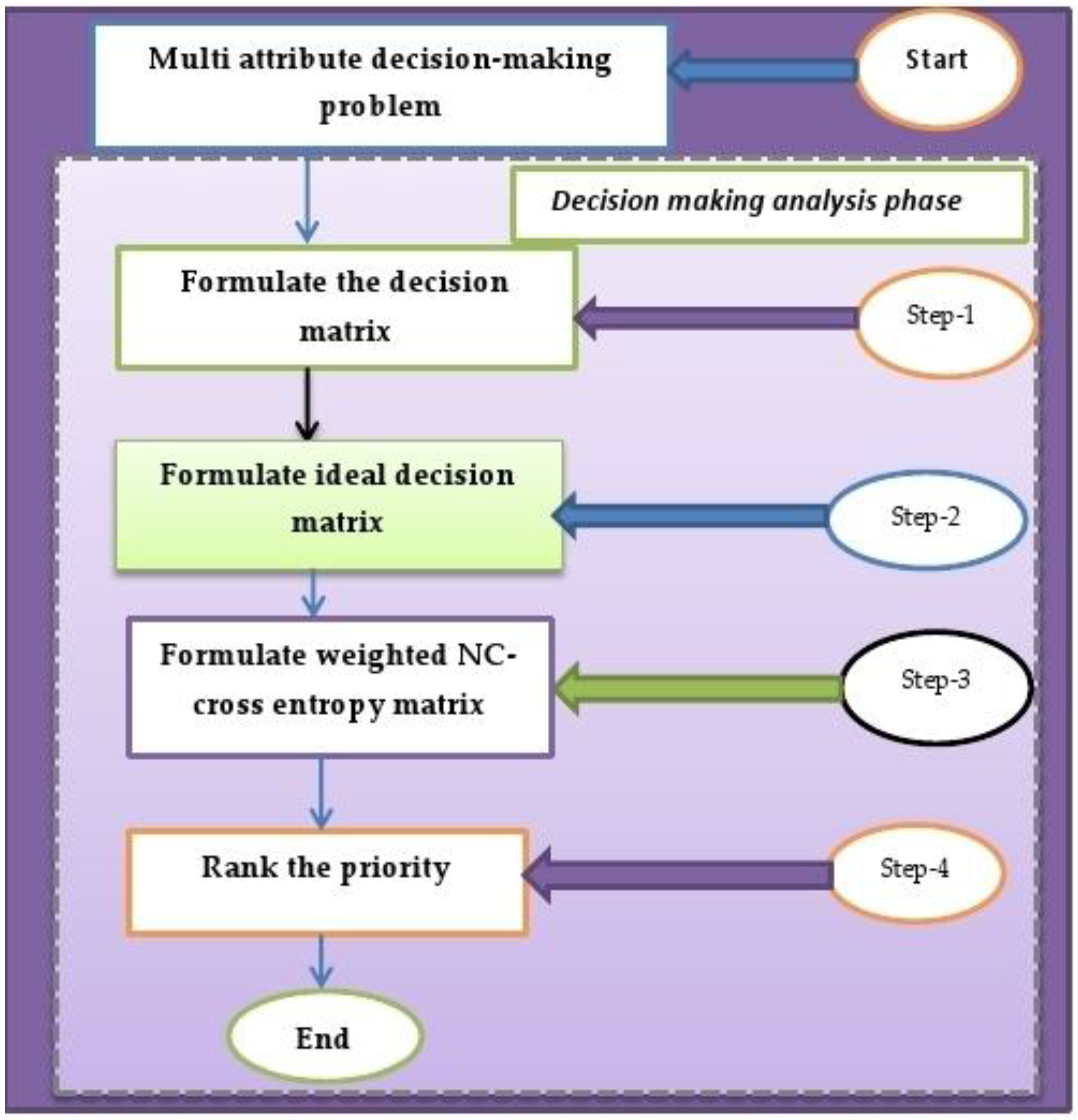
A conceptual model of the proposed strategy is shown in Figure 1.

5. Illustrative Example

In this section, we solve an illustrative example of an MADM problem to reflect the feasibility and efficiency of the proposed strategy in NCSs environments.

Now, we use an example [89] for cultivation and analysis. A venture capital firm intends to make evaluation and selection to five enterprises with the investment potential:

(1)

Automobile company (A₁)

(2)

Military manufacturing enterprise (A₂)

(3)

TV media company (A₃)

(4)

Food enterprises (A₄)

(5)

Computer software company (A₅)

On the basis of four attributes namely:

(1)

Social and political factor (G₁)

(2)

The environmental factor (G₂)

(3)

Investment risk factor (G₃)

(4)

The enterprise growth factor (G₄).

Weight vector of attributes is $\mathrm{W}=\{0.24, 0.25, 0.23, 0.28\}.$

The steps of decision-making strategy to rank alternatives are presented as follows:

Step 1. Formulate the decision matrix

The decision-maker represents the rating values of alternative Ai (i = 1, 2, 3, 4, 5) with respect to the attribute Gj (j = 1, 2, 3, 4) in terms of NCNs and constructs the decision matrix M as follows:

$$\mathrm{M}=\left(\begin{array}{ccccc}& {\mathrm{G}}_1& {\mathrm{G}}_2& {\mathrm{G}}_3& {\mathrm{G}}_4\\ {\mathrm{A}}_1& < [0.6, 0.8], [0.2, 0.3], [0.3,0.4 ],(0.8,0.3 , 0.4)>& <[0.5, 0.6], [0.2, 0.4], [0.4, 0.4],(0.6, 0.4, 0.4)>& <[0.6, 0.8], [0.2,0.3 ], [0.2,0.4 ],(0.8,0.4 ,0.4 )>& <[0.6, 0.7], [0.3,0.4 ], [0.3, 0.4 ],(0.7, 0.4, 0.5)>\\ {\mathrm{A}}_2& < [0.5, 0.7], [0.2, 0.3], [0.3,0.4 ],(0.7,0.3 , 0.4)>& <[0.7, 0.8], [0.2, 0.3], [0.2, 0.4],(0.8, 0.3, 0.4)>& <[0.6, 0.8], [0.2,0.4 ], [0.3,0.4 ],(0.8,0.4 ,0.4 )>& <[0.6, 0.8], [0.2,0.3 ], [0.2, 0.3 ],(0.8, 0.2, 0.3)>\\ {\mathrm{A}}_3& < [0.6, 0.8], [0.2, 0.4], [0.3,0.4 ],(0.8,0.4 , 0.4)>& <[0.6, 0.8], [0.2, 0.3], [0.2, 0.3],(0.8, 0.3, 0.3)>& <[0.8, 0.9], [0.3,0.5 ], [0.3,0.5 ],(0.9,0.5 ,0.5 )>& <[0.6, 0.7], [0.2,0.3 ], [0.2, 0.4 ],(0.7, 0.3, 0.4)>\\ {\mathrm{A}}_4& < [0.5, 0.7], [0.4, 0.5], [0.3,0.5 ],(0.7,0.5 , 0.5)>& <[0.4, 0.6], [0.1, 0.3], [0.3, 0.4],(0.6, 0.3, 0.4)>& <[0.5, 0.6], [0.1,0.2 ], [0.3,0.4 ],(0.6,0.2 ,0.4 )>& <[0.5, 0.7], [0.3,0.4 ], [0.4, 0.5 ],(0.7, 0.4, 0.5)>\\ {\mathrm{A}}_5& < [0.7, 0.8], [0.2, 0.4], [0.2,0.3 ],(0.8,0.4 , 0.4)>& <[0.4, 0.6], [0.2, 0.4], [0.2, 0.4],(0.6, 0.4, 0.4)>& <[0.5, 0.7], [0.2,0.4 ], [0.3,0.4 ],(0.7,0.4 ,0.4 )>& <[0.6, 0.8], [0.4,0.5 ], [0.4, 0.5 ],(0.8, 0.5, 0.5)>\end{array}\right).$$

(60)

Step 2. Formulate priori/ideal decision matrix

Priori/ideal decision matrix

$${\mathrm{M}}^1=\left(\begin{array}{ccccc}& {\mathrm{G}}_1& {\mathrm{G}}_2& {\mathrm{G}}_3& {\mathrm{G}}_4\\ {\mathrm{A}}_1& < [1, 1], [0, 0], [0,0 ],(1,0 , 0)>& <[1, 1], [0, 0], [0, 0],(1, 0, 0)>& <[1, 1], [0,0 ], [0,0 ],(1,0 ,0 )>& <[1, 1], [0,0 ], [0, 0 ],(1, 0, 0)>\\ {\mathrm{A}}_2& < [1, 1], [0, 0], [0,0 ],(1,0 , 0)>& <[1, 1], [0, 0], [0, 0],(1, 0, 0)>& <[1, 1], [0,0 ], [0,0 ],(1,0 ,0 )>& <[1, 1], [0,0 ], [0, 0 ],(1, 0, 0)>\\ {\mathrm{A}}_3& < [1, 1], [0, 0], [0,0 ],(1,0 , 0)>& <[1, 1], [0, 0], [0, 0],(1, 0, 0)>& <[1, 1], [0,0 ], [0,0 ],(1,0 ,0 )>& <[1, 1], [0,0 ], [0, 0 ],(1, 0, 0)>\\ {\mathrm{A}}_4& <[1, 1], [0,0 ], [0, 0 ],(1, 0, 0)>& <[1, 1], [0,0 ], [0, 0 ],(1, 0, 0)>& <[1, 1], [0,0 ], [0, 0 ],(1, 0, 0)>& <[1, 1], [0,0 ], [0, 0 ],(1, 0, 0)>\\ {\mathrm{A}}_5& <[1, 1], [0,0 ], [0, 0 ],(1, 0, 0)>& <[1, 1], [0,0 ], [0, 0 ],(1, 0, 0)>& <[1, 1], [0,0 ], [0, 0 ],(1, 0, 0)>& <[1, 1], [0,0 ], [0, 0 ],(1, 0, 0)>\end{array}\right).$$

(61)

Step 3. Calculate the weighted INS cross entropy matrix

Using Equation (38), we calculate weighted NC-cross entropy values between ideal matrixes (61) and decision matrix (60):

$${}^{\mathrm{N}\mathrm{C}}\mathrm{M}_{\mathrm{C}\mathrm{E}}^{\mathrm{w}}=\left(\begin{array}{l}0.66\\ 0.58\\ 0.60\\ 0.74\\ 0.71\end{array}\right).$$

(62)

Step 4. Rank the priority

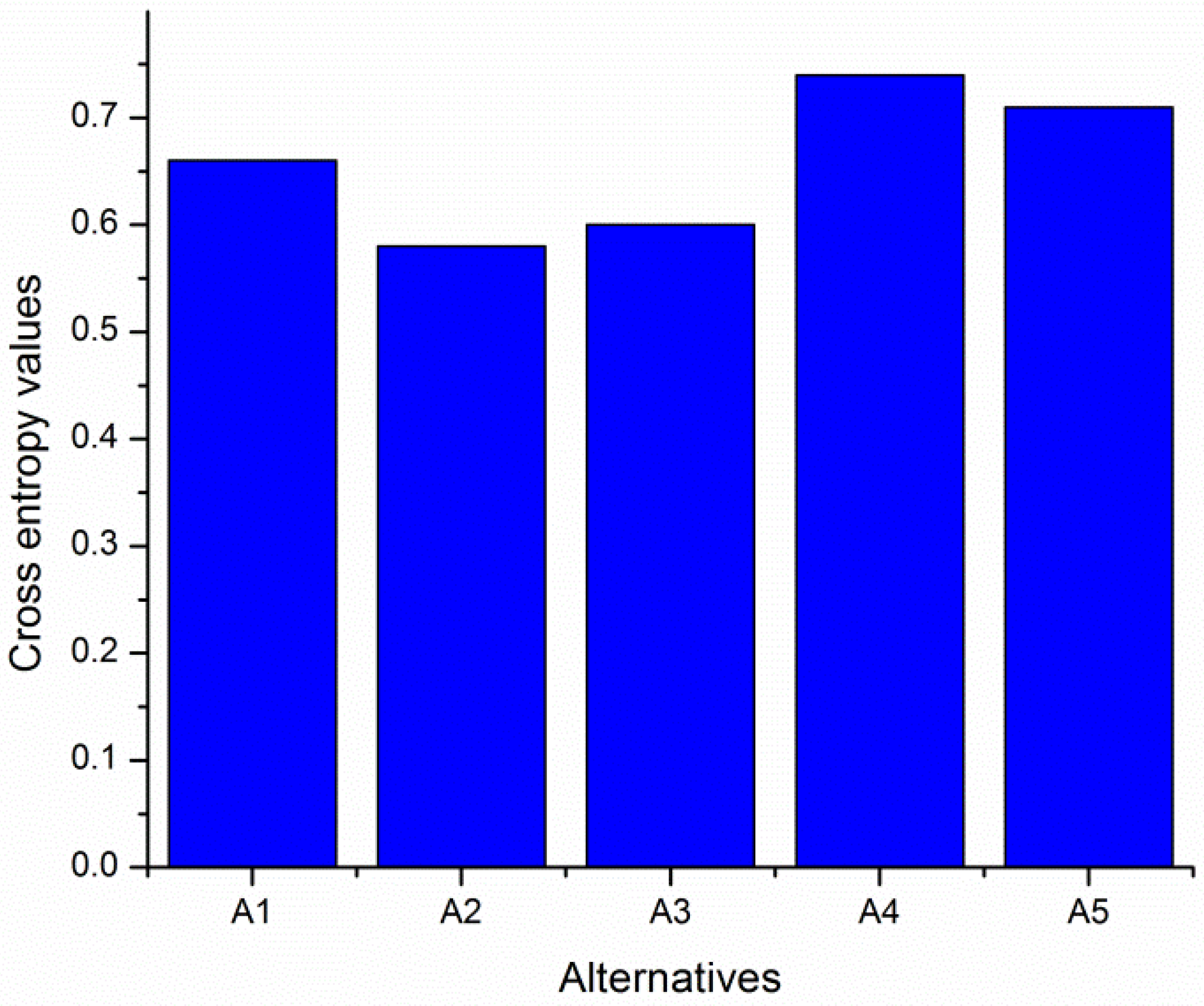
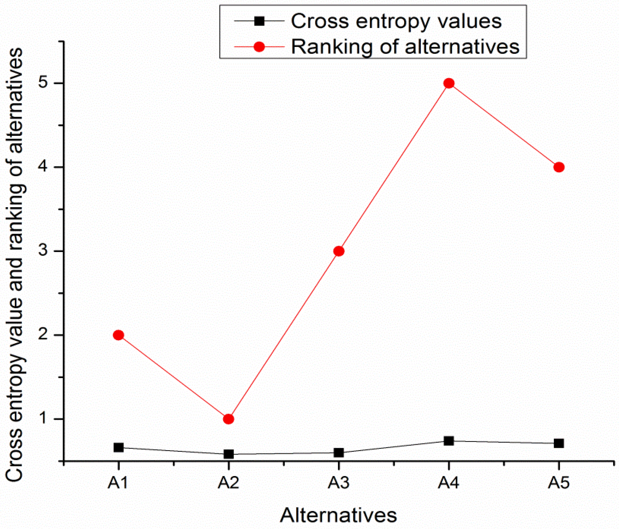
The position of cross entropy values of alternatives arranging in increasing order is 0.58 < 0.60 < 0.66 < 0.71 < 0.74. Since the smallest values of cross entropy indicate that the alternative is closer to the ideal alternative, the ranking priority of alternatives is A₂ > A₃ > A₁ > A₅ > A₄. Hence, military manufacturing enterprise (A₂) is the best alternative for investment.

Graphical representation of alternatives versus cross entropy is shown in Figure 2. From the Figure 2, we see that A₂ is the best preference alternative and A₄ is the least preference alternative.

Figure 3 presents relation between cross entropy value and preference ranking of the alternative.

6. Contributions of the Paper

The contributions of the paper are summarized as follows:

• We have introduced an NC-cross entropy measure and proved its basic properties in NCS environments.
• We have introduced a weighted NC-cross entropy measure and proved its basic properties in NCS environments.
• We have developed a novel MADM strategy based on weighted NC- cross entropy to solve MADM problems.
• We solved an illustrative example of MADM problem using proposed strategies.

7. Conclusions

We have introduced NC-cross entropy measure in NCS environments. We have proved the basic properties of the proposed NC-cross entropy measure. We have also introduced weighted NC-cross entropy measure and established its basic properties. Using the weighted NC-cross entropy measure, we developed a novel MADM strategy. We have also solved an MADM problem to illustrate the proposed MADM strategy. The proposed NC-cross entropy based MADM strategy can be employed to solve a variety of problems such as logistics center selection [90,91], weaver selection [92], teacher selection [21], brick selection [93], renewable energy selection [94], etc. The proposed NC-cross entropy based MADM strategy can also be extended to MAGDM strategy using suitable aggregation operators.

References

1. Smarandache, F. Neutrosophy, Neutrosophic Probability, Set, and Logic; American Research Press: Rehoboth, DE, USA, 1998. [Google Scholar]
2. Wang, H.; Smarandache, F.; Zhang, Y.; Sunderraman, R. Single valued neutrosophic sets. Multi-Space Multi-Struct. 2010, 4, 410–413. [Google Scholar]
3. Ansari, A.Q.; Biswas, R.; Aggarwal, S. Proposal for applicability of neutrosophic set theory in medical AI. Int. J. Comput. Appl. 2011, 27, 5–11. [Google Scholar] [CrossRef]
4. Guo, Y.; Cheng, H. New neutrosophic approach to image segmentation. Pattern Recognit. 2009, 42, 587–595. [Google Scholar] [CrossRef]
5. Cheng, H.D.; Guo, Y.; Zhang, Y. A novel image segmentation approach based on neutrosophic set and improved fuzzy c-mean algorithm. New Math. Nat. Comput. 2011, 7, 155–171. [Google Scholar] [CrossRef]
6. Guo, Y.; Sengur, A.; Ye, J. A novel image thresholding algorithm based on neutrosophic similarity score. Measurement 2014, 58, 175–186. [Google Scholar] [CrossRef]
7. Guo, Y.; Sengur, A. A novel image segmentation algorithm based on neutrosophic similarity clustering. Appl. Soft Comput. 2014, 25, 391–398. [Google Scholar] [CrossRef]
8. Guo, Y.; Sengur, A.; Tain, J. A novel breast ultrasound image segmentation algorithm based on neutrosophic similarity score and level set. Comput. Methods Programs Biomed. 2016, 123, 43–53. [Google Scholar] [CrossRef] [PubMed]
9. Mathew, J.; Simon, P. Color texture image segmentation based on neutrosophic set and nonsubsampled contourlet transformation. In Proceedings of the International Conference on Applied Algorithms, Kolkata, India, 13–15 January 2014; pp. 164–173. [Google Scholar]
10. Kraipeerapun, P.; Fung, C.C.; Brown, W. Assessment of uncertainty in mineral prospectivity prediction using interval neutrosophic sets. In Computational Intelligence and Security, Proceedings of the International Conference on Computational and Information Science, Xian, China, 15–19 December 2005; Springer: Berlin/Heidelberg, Germany, 2005; Volume 3802, pp. 1074–1079. [Google Scholar]
11. Kraipeerapun, P.; Fung, C.C. Binary classification using ensemble networks and interval neutrosophic sets. Neurocomputing 2009, 72, 2845–2856. [Google Scholar] [CrossRef]
12. Pramanik, S.; Chakrabarti, S. A study on problems of construction workers in West Bengal based on neutrosophic cognitive maps. Int. J. Innov. Res. Sci. Eng. Technol. 2013, 2, 6387–6394. [Google Scholar]
13. Kandasamy, W.B.V.; Smarandache, F. Fuzzy Cognitive Maps and Neutrosophic Cognitive Map; Xiquan: Phoenix, AZ, USA, 2003. [Google Scholar]
14. Mondal, K.; Pramanik, S. A study on problems of Hijras in West Bengal based on neutrosophic cognitive maps. Neutrosophic Sets Syst. 2014, 5, 21–26. [Google Scholar]
15. Pramanik, S.; Roy, T.K. Neutrosophic game theoretic approach to Indo-Pak conflict over Jammu-Kashmir. Neutrosophic Sets Syst. 2014, 2, 82–101. [Google Scholar]
16. Pramanik, S.; Roy, T.K. Game theoretic model to the Jammu-Kashmir conflict between India and Pakistan. Int. J. Math. Arch. 2013, 4, 162–170. [Google Scholar]
17. Sodenkamp, S. Models, Methods and Applications of Group Multiple-Criteria Decision Analysis in Complex and Uncertain Systems. Ph.D. Dissertation, University of Paderborn, Paderborn, Germany, 2013. [Google Scholar]
18. Biswas, P. Multi-Attribute Decision Making in Neutrosophic Environment. Ph.D. Dissertation, Jadavpur University, Kolkata, India, 19 February 2018. [Google Scholar]
19. Kharal, A. A neutrosophic multi-criteria decision-making method. New Math. Nat. Comput. 2014, 10, 143–162. [Google Scholar] [CrossRef]
20. Mondal, K.; Pramanik, S. Multi-criteria group decision-making approach for teacher recruitment in higher education under simplified neutrosophic environment. Neutrosophic Sets Syst. 2014, 6, 28–34. [Google Scholar]
21. Pramanik, S.; Mukhopadhyaya, D. Grey relational analysis-based intuitionistic fuzzy multi-criteria group decision-making approach for teacher selection in higher education. Int. J. Comput. Appl. 2011, 34, 21–29. [Google Scholar]
22. Mondal, K.; Pramanik, S. Neutrosophic decision-making model of school choice. Neutrosophic Sets Syst. 2015, 7, 62–68. [Google Scholar]
23. Mondal, K.; Pramanik, S. Neutrosophic decision-making model for clay-brick selection in construction field based on grey relational analysis. Neutrosophic Sets Syst. 2015, 9, 72–79. [Google Scholar]
24. Biswas, P.; Pramanik, S.; Giri, B.C. TOPSIS method for multi-attribute group decision-making under single valued neutrosophic environment. Neural Comput. Appl. 2016, 27, 727–737. [Google Scholar] [CrossRef]
25. Biswas, P.; Pramanik, S.; Giri, B.C. Entropy based grey relational analysis method for multi-attribute decision-making under single valued neutrosophic assessments. Neutrosophic Sets Syst. 2014, 2, 102–110. [Google Scholar]
26. Biswas, P.; Pramanik, S.; Giri, B.C. A new methodology for neutrosophic multi-attribute decision-making with unknown weight information. Neutrosophic Sets Syst. 2014, 3, 42–50. [Google Scholar]
27. Jiang, W.; Shou, Y. A novel single-valued neutrosophic set similarity measure and its application in multi criteria decision-making. Symmetry 2017, 9, 127. [Google Scholar] [CrossRef]
28. Mondal, K.; Pramanik, S. Neutrosophic tangent similarity measure and its application to multiple attribute decision-making. Neutrosophic Sets Syst. 2015, 9, 85–92. [Google Scholar]
29. Ye, J.; Zhang, Q.S. Single valued neutrosophic similarity measures for multiple attribute decision making. Neutrosophic Sets Syst. 2014, 2, 48–54. [Google Scholar]
30. Broumi, S.; Smarandache, F. Several similarity measures of neutrosophic sets. Neutrosophic Sets Syst. 2013, 1, 54–62. [Google Scholar]
31. Ye, J. Projection and bidirectional projection measures of single valued neutrosophic sets and their decision—Making method for mechanical design scheme. J. Exp. Theor. Artif. Intell. 2016. [Google Scholar] [CrossRef]
32. Sahin, R.; Liu, P. Maximizing deviation method for neutrosophic multiple attribute decision-making with incomplete weight information. Neural Comput. Appl. 2016, 27, 2017–2029. [Google Scholar] [CrossRef]
33. Ji, P.; Wang, J.Q.; Zhang, H.Y. Frank prioritized Bonferroni mean operator with single-valued neutrosophic sets and its application in selecting third-party logistics providers. Neural Comput. Appl. 2016. [Google Scholar] [CrossRef]
34. Nancy, H.G. Some new biparametric distance measures on single-valued neutrosophic sets with applications to pattern recognition and medical diagnosis. Information 2017, 8, 162. [Google Scholar] [CrossRef]
35. Sun, R.; Hu, J.; Chen, X. Novel single-valued neutrosophic decision-making approaches based on prospect theory and their applications in physician selection. Soft Comput. 2017. [Google Scholar] [CrossRef]
36. Stanujkic, D.; Zavadskas, E.K.; Smarandache, F.; Brauers, W.K.M.; Karabasevic, D. A neutrosophic extension of the MULTIMOORA Method. Informatica 2017, 28, 181–192. [Google Scholar] [CrossRef]
37. Zavadskas, E.K.; Baušys, R.; Stanujkic, D. Selection of lead-zinc flotation circuit design by applying WASPAS method with single-valued neutrosophic set. Acta Montan. Slovaca 2016, 21, 85–92. [Google Scholar]
38. Zavadskas, E.K.; Bausys, R.; Lazauskas, M. Sustainable assessment of alternative sites for the construction of a waste incineration plant by applying WASPAS method with single-valued neutrosophic set. Sustainability 2015, 7, 15923–15936. [Google Scholar] [CrossRef]
39. Bausys, R.; Zavadskas, E.K.; Kaklauskas, A. Application of neutrosophic set to multicriteria decision-making by COPRAS. J. Econ. Comput. Econ. Cybern. Stud. Res. 2015, 49, 91–106. [Google Scholar]
40. Xu, D.S.; Wei, C.G.W. TODIM method for single-valued neutrosophic multiple attribute decision-making. Information 2017, 8, 125. [Google Scholar] [CrossRef]
41. Ji, P.; Zhang, H.Y.; Wang, J.Q. A projection-based TODIM method under multi-valued neutrosophic environments and its application in personnel selection. Neural Comput. Appl. 2018, 29, 221–234. [Google Scholar] [CrossRef]
42. Peng, J.J.; Wang, J.Q.; Zhang, H.Y.; Chen, X.H. An outranking approach for multi-criteria decision-making problems with simplified neutrosophic sets. Appl. Soft Comput. 2014, 25, 336–346. [Google Scholar] [CrossRef]
43. Abdel-Basset, M.; Mohamed, M.; Smarandache, F. An extension of neutrosophic AHP–SWOT analysis for strategic planning and decision-making. Symmetry 2018, 10, 116. [Google Scholar] [CrossRef]
44. Pouresmaeil, H.; Shivanian, E.; Khorram, E.; Fathabadi, H.S. An extended method using TOPSIS and VIKOR for multiple attribute decision-making with multiple decision-makers and single valued neutrosophic numbers. Adv. Appl. Stat. 2017, 50, 261–292. [Google Scholar] [CrossRef]
45. Wang, H.; Smarandache, F.; Zhang, Y.Q.; Sunderraman, R. Interval Neutrosophic Sets and Logic: Theory and Applications in Computing; Hexis: Phoenix, AZ, USA, 2005. [Google Scholar]
46. Pramanik, S.; Mondal, K. Interval neutrosophic multi-attribute decision-making based on grey relational analysis. Neutrosophic Sets Syst. 2015, 9, 13–22. [Google Scholar]
47. Dey, P.P.; Pramanik, S.; Giri, B.C. An extended grey relational analysis based multiple attribute decision-making in interval neutrosophic uncertain linguistic setting. Neutrosophic soft multi-attribute decision-making based on grey relational projection method. Neutrosophic Sets Syst. 2016, 11, 21–30. [Google Scholar]
48. Dey, P.P.; Pramanik, S.; Giri, B.C. Extended projection-based models for solving multiple attribute decision-making problems with interval-valued neutrosophic information. In New Trends in Neutrosophic Theory and Applications; Smarandache, F., Pramanik, S., Eds.; Pons Editions: Brussels, Belgium, 2016; pp. 127–140. [Google Scholar]
49. Huang, Y.; Wei, G.W.; Wei, C. VIKOR method for interval neutrosophic multiple attribute group decision-making. Information 2017, 8, 144. [Google Scholar] [CrossRef]
50. Broumi, S.; Ye, J.; Smarandache, F. An extended TOPSIS method for multiple attribute decision-making based on interval neutrosophic uncertain linguistic variables. Neutrosophic Sets Syst. 2015, 8, 23–32. [Google Scholar]
51. Nancy, H.G. Non-linear programming method for multi-criteria decision-making problems under interval neutrosophic set environment. Appl. Intell. 2017. [Google Scholar] [CrossRef]
52. Zhang, H.Y.; Wang, J.Q.; Chen, X.H. An outranking approach for multi-criteria decision-making problems with interval-valued neutrosophic sets. Neural Comput. Appl. 2016, 27, 615–627. [Google Scholar] [CrossRef]
53. Pramanik, S.; Biswas, P.; Giri, B.C. Hybrid vector similarity measures and their applications to multi-attribute decision-making under neutrosophic environment. Neural Comput. Appl. 2017, 28, 1163–1176. [Google Scholar] [CrossRef]
54. Mondal, K.; Pramanik, S.; Giri, B.C. Interval neutrosophic tangent similarity measure based MADM strategy and its application to MADM Problems. Neutrosophic Sets Syst. 2018, 19. in press. [Google Scholar]
55. Ye, J. Similarity measures between interval neutrosophic sets and their applications in multi criteria decision-making. J. Intell. Fuzzy Syst. 2014, 26, 165–172. [Google Scholar]
56. Zhang, H.; Ji, P.; Wang, J.; Chen, X. An Improved weighted correlation coefficient based on integrated weight for interval neutrosophic sets and its application in multi criteria decision-making problems. Int. J. Comput. Intell. Syst. 2015, 8, 1027–1043. [Google Scholar] [CrossRef]
57. Zhao, A.W.; Du, J.G.; Guan, H.J. Interval valued neutrosophic sets and multi-attribute decision-making based on generalized weighted aggregation operator. J. Intell. Fuzzy Syst. 2015, 29, 2697–2706. [Google Scholar]
58. Smarandache, F.; Pramanik, S. (Eds.) New Trends in Neutrosophic Theory and Applications; Pons Editions: Brussels, Belgium, 2016; pp. 15–161. ISBN 978-1-59973-498-9. [Google Scholar]
59. Ali, M.; Deli, I.; Smarandache, F. The theory of neutrosophic cubic sets and their applications in pattern recognition. J. Intell. Fuzzy Syst. 2016, 30, 1957–1963. [Google Scholar] [CrossRef]
60. Banerjee, D.; Giri, B.C.; Pramanik, S.; Smarandache, F. GRA for multi attribute decision-making in neutrosophic cubic set environment. Neutrosophic Sets Syst. 2017, 15, 60–69. [Google Scholar]
61. Pramanik, S.; Dey, P.P.; Giri, B.C.; Smarandache, F. An Extended TOPSIS for multi-attribute decision-making problems with neutrosophic cubic information. Neutrosophic Sets Syst. 2017, 17, 20–28. [Google Scholar]
62. Zhan, J.; Khan, M.; Gulistan, M. Applications of neutrosophic cubic sets in multi-criteria decision-making. Int. J. Uncertain. Quantif. 2017, 7, 377–394. [Google Scholar] [CrossRef]
63. Lu, Z.; Ye, J. Cosine measures of neutrosophic cubic sets for multiple attribute decision-making. Symmetry 2017, 9, 121. [Google Scholar]
64. Shi, L.; Ye, J. Dombi aggregation operators of neutrosophic cubic sets for multiple attribute decision-making. Algorithms 2018, 11, 29. [Google Scholar] [CrossRef]
65. Ye, J. Linguistic neutrosophic cubic numbers and their multiple attribute decision-making method. Information 2017, 8, 110. [Google Scholar] [CrossRef]
66. Pramanik, S.; Dalapati, S.; Alam, S.; Roy, T.K.; Smarandache, F. Neutrosophic cubic MCGDM method based on similarity measure. Neutrosophic Sets Syst. 2017, 16, 44–56. [Google Scholar]
67. Pramanik, S.; Dalapati, S.; Alam, S.; Roy, T.K. NC-TODIM-based MAGDM under a neutrosophic cubic set environment. Information 2017, 8, 149. [Google Scholar] [CrossRef]
68. Pramanik, S.; Dalapati, S.; Alam, S.; Roy, T.K. NC-VIKOR based MAGDM under neutrosophic cubic set environment. Neutrosophic Sets Syst. 2018, 19. in press. [Google Scholar]
69. Zadeh, L.A. Probability measures of fuzzy events. J. Math. Anal. Appl. 1968, 23, 421–427. [Google Scholar] [CrossRef]
70. De Luca, A.; Termini, S. A definition of non-probabilistic entropy in the setting of fuzzy sets theory. Inf. Control 1972, 20, 301–312. [Google Scholar] [CrossRef]
71. Shannon, C.E. A mathematical theory of communication. Bell. Syst. Tech. J. 1948, 27, 379–423. [Google Scholar] [CrossRef]
72. Szmidt, E.; Kacprzyk, J. Entropy for intuitionistic fuzzy sets. Fuzzy Sets Syst. 2001, 118, 467–477. [Google Scholar] [CrossRef]
73. Majumder, P.; Samanta, S.K. On similarity and entropy of neutrosophic sets. J. Intell. Fuzzy Syst. 2014, 26, 1245–1252. [Google Scholar]
74. Aydoğdu, A. On entropy and similarity measure of interval valued neutrosophic sets. Neutrosophic Sets Syst. 2015, 9, 47–49. [Google Scholar]
75. Ye, J.; Du, S. Some distances, similarity and entropy measures for interval valued neutrosophic sets and their relationship. Int. J. Mach. Learn. Cybern. 2017. [Google Scholar] [CrossRef]
76. Shang, X.G.; Jiang, W.S. A note on fuzzy information measures. Pattern Recognit. Lett. 1997, 18, 425–432. [Google Scholar] [CrossRef]
77. Vlachos, I.K.; Sergiadis, G.D. Intuitionistic fuzzy information applications to pattern recognition. Pattern Recognit. Lett. 2007, 28, 197–206. [Google Scholar] [CrossRef]
78. Ye, J. Multicriteria fuzzy decision-making method based on the intuitionistic fuzzy cross-entropy. In Proceedings of the International Conference on Intelligent Human-Machine Systems and Cybernetics, Hangzhou, China, 26–27 August 2009; pp. 59–61. [Google Scholar]
79. Maheshwari, S.; Srivastava, A. Application of intuitionistic fuzzy cross entropy measure in decision-making for medical diagnosis. World Acad. Sci. Eng. Technol. Int. J. Math. Comput. Phys. Electr. Comput. Eng. 2015, 9, 254–258. [Google Scholar]
80. Zhang, Q.S.; Jiang, S.; Jia, B.; Luo, S. Some information measures for interval-valued intuitionistic fuzzy sets. Inf. Sci. 2010, 180, 5130–5145. [Google Scholar] [CrossRef]
81. Ye, J. Fuzzy cross entropy of interval valued intuitionistic fuzzy sets and its optimal decision-making method based on the weights of alternatives. Expert Syst. Appl. 2011, 38, 6179–6183. [Google Scholar] [CrossRef]
82. Ye, J. Single valued neutrosophic cross-entropy for multi criteria decision-making problems. Appl. Math. Model. 2013, 38, 1170–1175. [Google Scholar] [CrossRef]
83. Ye, J. Improved cross entropy measures of single valued neutrosophic sets and interval neutrosophic sets and their multi criteria decision-making methods. Cybern. Inf. Technol. 2015, 15, 13–26. [Google Scholar] [CrossRef]
84. Tian, Z.P.; Zhang, H.Y.; Wang, J.; Wang, J.Q.; Chen, X.H. Multi-criteria decision-making method based on a cross-entropy with interval neutrosophic sets. Int. J. Syst. Sci. 2016, 47, 3598–3608. [Google Scholar] [CrossRef]
85. Sahin, R. Cross-entropy measure on interval neutrosophic sets and its applications in multi criteria decision-making. Neural Comput. Appl. 2017, 28, 1177–1187. [Google Scholar] [CrossRef]
86. Pramanik, S.; Dalapati, S.; Alam, S.; Smarandache, F.; Roy, T.K. NS-Cross Entropy-Based MAGDM under Single-Valued Neutrosophic Set Environment. Information 2018, 9, 37. [Google Scholar] [CrossRef]
87. Dalapati, S.; Pramanik, S.; Alam, S.; Smarandache, F.; Roy, T.K. IN-cross entropy based MAGDM strategy under interval neutrosophic set environment. Neutrosophic Sets Syst. 2017, 18, 43–57. [Google Scholar] [CrossRef]
88. Pramanik, S.; Dey, P.P.; Smarandache, F.; Ye, J. Cross entropy measures of bipolar and interval bipolar neutrosophic sets and their application for multi-attribute decision-making. Axioms 2018, 7, 21. [Google Scholar] [CrossRef]
89. He, X.; Liu, W.F. An intuitionistic fuzzy multi-attribute decision-making method with preference on alternatives. Oper. Res. Manag. Sci. 2013, 22, 36–40. [Google Scholar]
90. Pramanik, S.; Dalapati, S.; Roy, T.K. Logistics center location selection approach based on neutrosophic multi-criteria decision-making. In New Trends in Neutrosophic Theory and Applications; Smarandache, F., Pramanik, S., Eds.; Pons Asbl: Brussels, Belgium, 2016; Volume 1, pp. 161–174. ISBN 978-1-59973-498-9. [Google Scholar]
91. Pramanik, S.; Dalapati, S.; Roy, T.K. Neutrosophic Multi-Attribute Group Decision Making Strategy for Logistics Center Location Selection. In Neutrosophic Operational Research Volume III; Smarandache, F., Basset, M.A., Chang, V., Eds.; Pons Asbl: Brussels, Belgium, 2018; pp. 13–32. ISBN 978-1-59973-537-5. [Google Scholar]
92. Dey, P.P.; Pramanik, S.; Giri, B.C. Multi-criteria group decision-making in intuitionistic fuzzy environment based on grey relational analysis for weaver selection in Khadi institution. J. Appl. Quant. Methods 2015, 10, 1–14. [Google Scholar]
93. Mondal, K.; Pramanik, S. Intuitionistic fuzzy multi criteria group decision-making approach to quality-brick selection problem. J. Appl. Quant. Methods 2014, 9, 35–50. [Google Scholar]
94. San Cristóbal, J.R. Multi-criteria decision-making in the selection of a renewable energy project in Spain: The VIKOR method. Renew. Energy 2011, 36, 498–502. [Google Scholar] [CrossRef]
Figure 1. A flow chart of the NC-cross entropy based MADM strategy.
Mathematics 06 00067 g001
Figure 2. Bar diagram of alternatives versus cross entropy values of alternatives.
Mathematics 06 00067 g002
Figure 3. Graphical representation of cross entropy values and ranking of alternatives.
Mathematics 06 00067 g003