A New Descent Algorithm Using the Three-Step Discretization Method for Solving Unconstrained Optimization Problems

Abstract

In this paper, three-step Taylor expansion, which is equivalent to third-order Taylor expansion, is used as a mathematical base of the new descent method. At each iteration of this method, three steps are performed. Each step has a similar structure to the steepest descent method, except that the generalized search direction, step length, and next iterative point are applied. Compared with the steepest descent method, it is shown that the proposed algorithm has higher convergence speed and lower computational cost and storage.

1. Introduction

We start our discussion by considering the unconstrained minimization problem:

$$\mathrm{Find}:{\mathbf{x}}^{*}={[x_1^{*},x_2^{*},\cdots ,x_n^{*}]}^T\mathrm{that}\mathrm{minimizes}f(x_1,x_2,\dots ,x_n)\equiv f(\mathbf{x}).$$

where f is an n-dimensional continuously differentiable function.

Most effective optimization procedures include some basic steps. At iteration k, where the current $\mathbf{x}$ is ${\mathbf{x}}_k$, they do the following:

1.

Specify the initial starting vector ${\mathbf{x}}^0={[x_1^0,x_2^0,\cdots ,x_n^0]}^T$,

2.

Find an appropriate search direction ${\mathbf{d}}_k$,

3.

Specify the convergence criteria for termination,

4.

Minimize along the direction ${\mathbf{d}}_k$ to find a new point ${\mathbf{x}}_{k+1}$ from the following equation

$${\mathbf{x}}_{k+1}={\mathbf{x}}_k+{\alpha }_k{\mathbf{d}}_k.$$

(1)

where ${\alpha }_k$ is a positive scalar called the step size. The step size is usually determined by an optimization process called a line search (usually inexactly) such as Wolfe-line search, Goldstein-line search or Armijo-line search

$$f({\mathbf{x}}_k+\alpha {\mathbf{d}}_k)<f({\mathbf{x}}_k)+\alpha c\nabla f({\mathbf{x}}_k).{\mathbf{d}}_k.$$

(2)

where $c\in (0,1)$ is a constant control parameter. For more information on the line search strategy, readers can refer to [1,2,3,4,5,6,7]. In addition, some researchers have introduced suitable algorithms which defined ${\alpha }_k$ without a line search method that can be seen in the literature [8,9,10]. Appropriate choices for an initial starting point have a positive effect on computational cost and speed of convergence.

The numerical optimization of general multivariable objective functions differs mainly in how they generate the search directions. A good search direction should reduce the objective function’s value so that

$$f({\mathbf{x}}_{k+1})<f({\mathbf{x}}_k).$$

Such a direction ${\mathbf{d}}_k$ is a descent direction and satisfies the following requirement at any point

$$\nabla f({\mathbf{x}}_k).{\mathbf{d}}_k<0$$

(3)

where the dot indicates the inner product of two vectors $\nabla f({\mathbf{x}}_k)$ and ${\mathbf{d}}_k$.

The choice of search direction ${\mathbf{d}}_k$ is typically based on some approximate model of the objective function f which is obtained by the Taylor series [11]

$$\begin{array}{cc}\hfill f(\mathbf{x}+\Delta \mathbf{x})=f(\mathbf{x})& +\nabla f(\mathbf{x}).\Delta \mathbf{x}+\frac{1}{2!}\nabla [\nabla f.\Delta \mathbf{x}].\Delta \mathbf{x}\hfill \\ \hfill & +\frac{1}{3!}\nabla [\nabla [\nabla f.\Delta \mathbf{x}].\Delta \mathbf{x}].\Delta \mathbf{x}+\cdots .\hfill \end{array}$$

(4)

where $\mathbf{x}$ and $\Delta \mathbf{x}$ are replaced with ${\mathbf{x}}_k$ and $\alpha {\mathbf{d}}_k$, respectively.

For instance, a linear approximation (first order Taylor expansion) of the objective function

$$f({\mathbf{x}}_k+\alpha {\mathbf{d}}_k)\approx f({\mathbf{x}}_k)+\alpha \nabla f({\mathbf{x}}_k).{\mathbf{d}}_k$$

can be used which concludes the following direction

$${\mathbf{d}}_k=-\nabla f({\mathbf{x}}_k).$$

This is referred to as the steepest descent method [4]. The overall results on the convergence of the steepest descent method can be found in [4,12,13]. More practical applications of the steepest descent method are discussed in [10,14,15,16].

Unlike gradient methods which use first order Taylor expansion, Newton method uses a second order Taylor expansion of the function about the current design point; i.e., a quadratic model

$$f({\mathbf{x}}_k+{\mathbf{d}}_k)\approx f({\mathbf{x}}_k)+\nabla f({\mathbf{x}}_k).{\mathbf{d}}_k+\frac{1}{2}\nabla [\nabla f({\mathbf{x}}_k).{\mathbf{d}}_k].{\mathbf{d}}_k.$$

which yields Newton direction

$${\mathbf{d}}_k=-({\nabla }^{2}f{({\mathbf{x}}_k)}^{-1}\nabla f({\mathbf{x}}_k).$$

Although the Newton method is below the quadratic rate of convergence, it requires the computation and storage of some matrices associated with the Hessian of the objective function. Moreover, the Newton method can only be utilized if the Hessian matrix is positive definite [4].

The purpose of this paper is to provide a descent algorithm which can exploit more information about the objective function without the need to store large matrices such as the Hessian matrix. In order to construct a desired model of the objective function, we propose a three-step discretization method based on three-step Taylor expansion that is used in [17,18,19] as follows

$$\begin{array}{c}\hfill \left\{\begin{array}{c}f(\mathbf{x}+{\displaystyle \frac{\Delta \mathbf{x}}{3}})\simeq f(\mathbf{x})+{\displaystyle \frac{1}{3}}\nabla f(\mathbf{x}).\Delta \mathbf{x}\hfill \\ f(\mathbf{x}+{\displaystyle \frac{\Delta \mathbf{x}}{2}})\simeq f(\mathbf{x})+{\displaystyle \frac{1}{2}}\nabla f(\mathbf{x}+{\displaystyle \frac{\Delta \mathbf{x}}{3}}).\Delta \mathbf{x}\hfill \\ f(\mathbf{x}+\Delta \mathbf{x})\simeq f(\mathbf{x})+\nabla f(\mathbf{x}+{\displaystyle \frac{\Delta \mathbf{x}}{2}}).\Delta \mathbf{x}.\hfill \end{array}\right.\end{array}$$

(5)

Formula (5) is equivalent to Equation (4) truncated at three terms, i.e.,

$$\begin{array}{cc}\hfill f(\mathbf{x}+\Delta \mathbf{x})=f(\mathbf{x})& +\nabla f(\mathbf{x}).\Delta \mathbf{x}+\frac{1}{2!}\nabla [\nabla f.\Delta \mathbf{x}].\Delta \mathbf{x}\hfill \\ \hfill & +\frac{1}{3!}\nabla [\nabla [\nabla f.\Delta \mathbf{x}].\Delta \mathbf{x}].\Delta \mathbf{x}+O[{(\Delta \mathbf{x})}^4].\hfill \end{array}$$

(6)

Hence, using these steps of Formula (5) in the approximation of a function around $\mathbf{x}$ gives a third-order accuracy with $O[{(\Delta \mathbf{x})}^4]$.

On the other hand, we can say that these steps of Formula (5) are derived by applying a factorization process to the right side of Equation (6) as follows

$$\begin{array}{cc}\hfill f(\mathbf{x})[\mathbf{I}& +\nabla .\Delta \mathbf{x}\left[\mathbf{I}+{\displaystyle \frac{1}{2}}\nabla .\Delta \mathbf{x}[\mathbf{I}+{\displaystyle \frac{1}{3}}\nabla .\Delta \mathbf{x}]\right]]\hfill \\ \hfill & =\left[f(\mathbf{x})+\nabla .\Delta \mathbf{x}\left[f(\mathbf{x})+{\displaystyle \frac{1}{2}}\nabla .\Delta \mathbf{x}[f(\mathbf{x})+{\displaystyle \frac{1}{3}}\nabla f(x).\Delta \mathbf{x}]\right]\right]+O[{(\Delta \mathbf{x})}^4].\hfill \end{array}$$

(7)

where the symbol $\mathbf{I}$ is the identity operator. Now, by removing the terms appearing in $O[{(\Delta \mathbf{x})}^4]$ and using the Taylor series properties, the first internal bracket in Equation (7) shows $f(\mathbf{x}+\frac{\Delta \mathbf{x}}{3})$, the second internal bracket shows $f(\mathbf{x}+\frac{\Delta \mathbf{x}}{2})$ and the last one shows $f(\mathbf{x}+\Delta \mathbf{x})$.

Jiang and Kawahara [17] are the pioneers who used this formula to solve unsteady incompressible flows governed by the Navier-Stokes equations. In their method, the discretization in time is performed before the spatial approximation by means of Formula (5) with respect to the time. In comparison with the Equation (6), Formula (5) does not contain any new higher-order derivatives. Moreover, it reduces the demand of smoothness of the function, gives the superior approximation of the function and presents some stability advantages in multidimensional problems [17]. The Formula (5) is useful in solving non-linear partial differential equations, hyperbolic problems, multi-dimensional and coupled equations.

In this article, we utilize Formula (5) to obtain a descent direction that satisfies the inequality of Equation (3) and then modify the Armijo-rule in the line search method to achieve an appropriate step size. Finally, Equation (1) is utilized to obtain a sequence that reduces the value of the function. Since all equations of the three-step discretization process involve only the first order derivative of the function, the proposed method is a member of gradient methods such as the steepest descent method. However, numerical results demonstrate that the current method works better than the steepest descent method.

The organization of the paper is as follows. In Section 2, there is a brief review of the gradient-type algorithms and their applications. In Section 3, the three-step discretization algorithm and its fundamental properties are described. In Section 4, we show how the proposed algorithm converges globally. Some noteworthy numerical examples are presented in Section 5. Finally, Section 6 provides conclusions of the study.

2. Related Work

This section provides an overview of previous research on the gradient-type methods.

2.1. Steepest Descent Method

Gradient descent is among the most popular algorithms to perform optimization. The steepest descent method, which can be traced back to Cauchy in 1847 [20], has a rich history and is regarded as the simplest and best-known gradient method. Despite its simplicity, the steepest descent method has played a major role in the development of the theory of optimization. Unfortunately, the classical steepest descent method which uses the exact line search procedure in determining the step size is known for being quite slow in most real-world problems and is therefore not widely used. Recently, several modifications to the steepest descent method have been presented to overcome its weakness. Mostly, these modifications propose effective trends in choosing the step length. Barzilai and Borwein (BB method) [21] presented a new choice of step length through the two-point step size

$${\alpha }_k={\displaystyle \frac{{\mathbf{s}}_{k-1}^T{\mathbf{y}}_{k-1}}{\parallel {\mathbf{y}}_{k-1}^T{\parallel }_2^2}},{\alpha }_k={\displaystyle \frac{\parallel {\mathbf{s}}_{k-1}^T{\parallel }_2^2}{{\mathbf{s}}_{k-1}^T{\mathbf{y}}_{k-1}}}.$$

where ${\mathbf{s}}_{k-1}={\mathbf{x}}_k-{\mathbf{x}}_{k-1}$ and ${\mathbf{y}}_{k-1}=\nabla {\mathbf{f}}_k-\nabla {\mathbf{f}}_{k-1}$.

Although their method did not guarantee the monotonic descent of the residual norms, the BB method was capable of performing quite well for high dimensional problems. The results of Barzilai and Borwein have encouraged many researchers to modify the steepest descent method. For instance, Dai and Fletcher in 2005 [22] used a new gradient projection method for box-constrained quadratic problems with the step length

$${\alpha }_k={\displaystyle \frac{\parallel {\mathbf{s}}_{k-\overline{m}}^T{\parallel }_2^2}{{\mathbf{s}}_{k-\overline{m}}^T{\mathbf{y}}_{k-\overline{m}}}}.$$

where $\overline{m}=min(m,k-1)$ and $m\ge 1$ is some prefixed integer.

Hassan et al. in 2009 [23] were motivated by the BB method and presented a Monotone gradient method via the Quasi-Cauchy relation. They discover a step length formula that approximates the inverse of Hessian using the Quasi-Cauchy equation which retains the monotonic property for every repetition. Leong et al. in 2010 [24] suggested a fixed step gradient type method to improve the BB method and it is recognized as the Monotone gradient method via the weak secant equation. In the Leong method, the approximation is stored using a diagonal matrix depending on the modified weak secant equation. Recently, Tan et al. in 2016 [25] applied the Barzilai and Borwein step length to the stochastic gradient descent and stochastic variance gradient algorithms.

Plenty of attention has also been paid to the theoretical properties of the BB method. Barzilai and Borwein [21] proved that the BB method has an R-superlinear convergence when the dimension is just two. For the general n-dimensional strong convex quadratic function, this method is also convergent and the convergence rate is R-linear [26,27]. Recently, Dai [28] presented a novel analysis of the BB method for two-dimensional strictly convex quadratic functions and showed that there is a superlinear convergence step in at most three consecutive steps.

Another modification method that implemented the choice of an efficient step length was proposed by Yuan [29]. He has suggested a new step size for the steepest descent method. The desired formula for the new ${\alpha }_k$ was obtained through an analysis of two-dimensional problems. In his proposed algorithm, this new step size was used in even iterations and the exact line search was used in odd iterations. Unlike the BB method, Yuan’s method possesses the monotonic property. For a constant k Yuan’s step size is defined as follows

$${\alpha }_{2k}={\displaystyle \frac{2}{\sqrt{{(1/{\alpha }_{2k-1}^{*}-1/{\alpha }_{2k}^{*})}^2+4\parallel \nabla {\mathbf{f}}_{2k}{\parallel }_2^2/{\parallel {\mathbf{s}}_{2k-1}\parallel }_2^2}+1/{\alpha }_{2k-1}^{*}+1/{\alpha }_{2k}^{*}}}.$$

where ${\alpha }_{2k-1}^{*}$ and ${\alpha }_{2k}^{*}$ are computed through the exact line search.

In addition to these mentioned modification algorithms, there is various literature which used different improvement style for the steepest descent method. For example, Manton [30] derived algorithms which minimize a cost function with the constraint condition by reducing the dimension of the optimization problem by reformulating the optimization problem as an unconstrained one on the Grassmann manifold. Zhou and Feng [10] proposed the steepest descent algorithm without the line search for the p-Laplacian problem. In their method, the search direction is the weighted preconditioned steepest descent one, and, with the exception of the first iteration, the step length is measured by a formula.

2.2. Newton Method

The steepest descent method lacks second derivative information, causing inaccuracy. Thus, some researchers have used a more effective method which is identified as the Newton method. Newton’s work was done in the year 1669, but it was published a few years later. For each iteration of the Newton method, we will need to compute the second derivative called the Hessian of a given function. It is difficult to calculate Hessian manually, especially when differentiation gets complicated. This will need a lot of computing effort and, in some cases, the second derivation cannot be computed analytically. Even for some simpler differentiation, it may be time-consuming. In addition, considerable storage space is needed to store the computed Hessian and this is computationally expensive. For example, if we have a Hessian with n dimensions, we will have $O(n^2)$ storage space to store the Hessian [31].

2.3. Conjugate Gradient Methods

Another gradient descent method is the conjugate gradient method. The conjugate gradient method has been considered an effective numerical method for solving large-scale unconstrained optimization problems because it does not need the storage of any matrices. The search direction of the conjugate gradient method is defined by

$$\begin{array}{c}\hfill {\mathbf{d}}_k=\left\{\begin{array}{c}-\nabla {\mathbf{f}}_k,k=0,\hfill \\ -\nabla {\mathbf{f}}_k+{\beta }_k\nabla {\mathbf{f}}_{k-1},k\ge 0,\hfill \end{array}\right.\end{array}$$

where ${\beta }_k$ is a parameter which characterizes the conjugate gradient method. There are many articles on how to get ${\beta }_k$. The Hestenes-Stiefel (HS) [32] and Fletcher-Reeves (FR) [33] are well-known formulas for obtaining this parameter which is respectively given by

$${\beta }_k^{HS}=\frac{\nabla {\mathbf{f}}_k^T{\mathbf{y}}_{k-1}}{{\mathbf{d}}_{k-1}^T{\mathbf{y}}_{k-1}},{\beta }_k^{FR}=\frac{\parallel \nabla {\mathbf{f}}_k^T{\parallel }_2^2}{\parallel \nabla {\mathbf{f}}_{K-1}^T{\parallel }_2^2}.$$

The global convergence properties of these methods have been shown in many research papers; for example, [34]. The classical conjugate gradient methods only include the first derivative of the function. In this decade, in order to incorporate the second-order information about the objective function into conjugate gradient methods, many researchers have proposed conjugate gradient methods based on secant conditions. Dai and Liao [35] proposed a conjugate gradient method based on the secant condition and proved its global convergence property. Kobayashi et al. [36] proposed conjugate gradient methods based on structured secant conditions for solving nonlinear least squares problems. Although numerical experiments of the previous research show the effectiveness of these methods for solving large-scale unconstrained optimization problems, these methods do not necessarily satisfy the descent condition. In order to overcome this deficiency, various authors present modifications of the conjugate gradient methods. For example, Zhang et al. [37] presented a modification to the FR method such that the direction generated by the modified method provides a descent direction. Sugiki et al. [38] proposed three-term conjugate gradient methods based on the secant conditions which always satisfy the sufficient descent condition.

3. New Descent Algorithm

In this section, we show how equations in Formula (5) can be used to propose the three-step discretization method and give its pseudo-code. The following regularity of $f(\mathbf{x})$ is assumed in the following:

Assumption 1.

We assume $f\in {\mathrm{C}}^1({\mathbb{R}}^n)$ with Lipschitz continuous gradient, i.e., there exists $L>0$ such that

$$\parallel \nabla f(\mathbf{x})-\nabla f(\mathbf{y})\parallel \le L\parallel \mathbf{x}-\mathbf{y}\parallel ,\forall \mathbf{x},\mathbf{y}\in {\mathbb{R}}^n.$$

The substitution $\alpha \mathbf{d}$ for $\Delta \mathbf{x}$ in Formula (5) yields:

$$\begin{array}{c}\hfill \left\{\begin{array}{c}f(\mathbf{x}+{\displaystyle \frac{\alpha \mathbf{d}}{3}})\simeq f(\mathbf{x})+{\displaystyle \frac{\alpha }{3}}\nabla f(\mathbf{x}).\mathbf{d}\hfill \\ f(\mathbf{x}+{\displaystyle \frac{\alpha \mathbf{d}}{2}})\simeq f(\mathbf{x})+{\displaystyle \frac{\alpha }{2}}\nabla f(\mathbf{x}+{\displaystyle \frac{\alpha \mathbf{d}}{3}}).\mathbf{d}\hfill \\ f(\mathbf{x}+\alpha \mathbf{d})\simeq f(\mathbf{x})+\alpha \nabla f(\mathbf{x}+{\displaystyle \frac{\alpha \mathbf{d}}{2}}).\mathbf{d}.\hfill \end{array}\right.\end{array}$$

(8)

3.1. Three-Step Discretization Algorithm

Three steps are performed throughout this algorithm. Actually, in the steepest descent method, there is not an intermediate step between the computation of ${\mathbf{x}}_k$ and ${\mathbf{x}}_{k+1}$. However, in the proposed method, we impose an intermediate step between ${\mathbf{x}}_k$ and ${\mathbf{x}}_{k+1}$. In other words, ${\mathbf{x}}_k$ is computed from the first step and ${\mathbf{x}}_{k+1}$ is computed from the third step. The second step is an intermediate step that uses ${\mathbf{x}}_k$ as the starting point and produces the new point such as ${\mathbf{x}}^{*}$. The ${\mathbf{x}}^{*}$ forms the starting point for the last step which results in ${\mathbf{x}}_{k+1}$. The structure of the proposed algorithm is characterized as follows.

The main goal of this algorithm is that the value of the objective function declines during all three steps. If the same direction is applied to all three steps, it will be a non-descent direction in at least one of the steps. Therefore, we need to consider each of the steps separately. Moreover, if the point ${\mathbf{x}}_k$ is employed in the first step of Formula (8), the point ${\mathbf{x}}_{k+1}$ will be achieved by the third step of Formula (8).

To determine which step of Formula (8) is performing, we use the super-index j. At each upgrading index k, the index j adopts only values $(0)$, $(1)$ and $(2)$, respectively. During the kth iteration of the main algorithm, directions ${\mathbf{d}}_k^{(0)}$, ${\mathbf{d}}_k^{(1)}$, and ${\mathbf{d}}_k^{(2)}$ are used in the first, second and third step, respectively. The points ${\mathbf{x}}_k^{(0)}$, ${\mathbf{x}}_k^{(1)}$, and ${\mathbf{x}}_k^{(2)}$ are used as starting points in the first, second and third step, respectively. The proper steps size ${\alpha }_k^{(0)}$, ${\alpha }_k^{(1)}$, and ${\alpha }_k^{(2)}$ are obtained from the first, second and last step, respectively. Details are explained as follows.

The first step of Formula (8) can be rewritten in the following form

$$f({\mathbf{x}}_k^{(0)}+{\displaystyle \frac{\alpha {\mathbf{d}}_k^{(0)}}{3}})\simeq f({\mathbf{x}}_k^{(0)})+{\displaystyle \frac{\alpha }{3}}\nabla f({\mathbf{x}}_k^{(0)}).{\mathbf{d}}_k^{(0)}.$$

The direction ${\mathbf{d}}_k^{(0)}$ should be chosen in such a way that $\nabla f({\mathbf{x}}_k^{(0)}).{\mathbf{d}}_k^{(0)}$ provides the greatest reduction in $f({\mathbf{x}}_k^{(0)})$ so that

$$f({\mathbf{x}}_k^{(0)}+{\displaystyle \frac{\alpha {\mathbf{d}}_k^{(0)}}{3}})<f({\mathbf{x}}_k^{(0)}).$$

Hence, the direction of the first step is calculated similarly to the process of finding steepest descent direction [4]. So, in the first step of Formula (8), we choose

$${\mathbf{d}}_k^{(0)}=-\nabla f({\mathbf{x}}_k^{(0)}).$$

Next, we must determine a proper step size for the first step. In this article, to find the step size, we use the backtracking algorithm with an Armijo-line search. Considering the first step of Formula (8), the general Armijo condition of Equation (2) can be modified as follows

$$f({\mathbf{x}}_k^{(0)}+\frac{\alpha }{3}{\mathbf{d}}_k^{(0)})<f({\mathbf{x}}_k^{(0)})+\frac{\alpha }{3}c\nabla f({\mathbf{x}}_k^{(0)}).{\mathbf{d}}_k^{(0)}.$$

(9)

Therefore, the implementation of the backtracking algorithm with Equation (9) provides the proper step size, ${\alpha }_k^{(0)}$, and the following point

$${\mathbf{x}}_k^{(1)}={\mathbf{x}}_k^{(0)}+{\displaystyle \frac{{\alpha }_k^{(0)}{\mathbf{d}}_k^{(0)}}{3}}.$$

(10)

We use ${\mathbf{x}}_k^{(1)}$ as a starting point for the second step of Formula (8).

We can rewrite the second step as follows:

$$f({\mathbf{x}}_k^{(1)}+{\displaystyle \frac{\alpha {\mathbf{d}}_k^{(1)}}{2}})\simeq f({\mathbf{x}}_k^{(1)})+{\displaystyle \frac{\alpha }{2}}\nabla f({\mathbf{x}}_k^{(0)}+{\displaystyle \frac{{\alpha }_k^{(0)}{\mathbf{d}}_k^{(0)}}{3}}).{\mathbf{d}}_k^{(1)}.$$

Now the direction ${\mathbf{d}}_k^{(1)}$ should satisfy the descent requirement of Equation (3) at the point, ${\mathbf{x}}_k^{(0)}+{\displaystyle \frac{{\alpha }_k^{(0)}{\mathbf{d}}_k^{(0)}}{3}}$, i.e.,

$$\nabla f({\mathbf{x}}_k^{(0)}+{\displaystyle \frac{{\alpha }_k^{(0)}{\mathbf{d}}_k^{(0)}}{3}}).{\mathbf{d}}_k^{(1)}<0.$$

By using a similar analysis for finding the steepest descent direction and using Equation (10) we have

$${\mathbf{d}}_k^{(1)}=-\nabla f({\mathbf{x}}_k^{(0)}+{\displaystyle \frac{{\alpha }_k^{(0)}{\mathbf{d}}_k^{(0)}}{3}})=-\nabla f({\mathbf{x}}_k^{(1)}).$$

(11)

After determining the direction ${\mathbf{d}}_k^{(1)}$, we should find a proper step size. In the second step, we modify general Armijo condition of Equation (2) as follows

$$f({\mathbf{x}}_k^{(1)}+\frac{\alpha }{2}{\mathbf{d}}_k^{(1)})<f({\mathbf{x}}_k^{(1)})+\frac{\alpha }{2}c\nabla f({\mathbf{x}}_k^{(1)}).{\mathbf{d}}_k^{(1)}.$$

(12)

We use Equation (12) in the backtracking algorithm to find the proper step size, ${\alpha }_k^{(1)}$, and the following point

$${\mathbf{x}}_k^{(2)}={\mathbf{x}}_k^{(1)}+\frac{{\alpha }_k^{(1)}{\mathbf{d}}_k^{(1)}}{2}.$$

(13)

We use the point ${\mathbf{x}}_k^{(2)}$ as a starting point in the last step of Formula (8).

Now, we have the following result in the third step

$$f({\mathbf{x}}_k^{(2)}+\alpha {\mathbf{d}}_k^{(2)})\simeq f({\mathbf{x}}_k^{(2)})+\alpha \nabla f({\mathbf{x}}_k^{(1)}+{\displaystyle \frac{{\alpha }_k^{(1)}{\mathbf{d}}_k^{(1)}}{2}}).{\mathbf{d}}_{\mathbf{k}}^{(2)}.$$

where the Equation (11) gives ${\mathbf{d}}_k^{(1)}$. The direction ${\mathbf{d}}_k^{(2)}$ is obtained from

$${\mathbf{d}}_k^{(2)}=-\nabla f({\mathbf{x}}_k^{(1)}+{\displaystyle \frac{{\alpha }_k^{(1)}{\mathbf{d}}_k^{(1)}}{2}})=-\nabla f({\mathbf{x}}_k^{(2)}).$$

Also, according to the last step of Formula (8), the last step of the presented algorithm uses the general Armijo condition of Equation (2). With replacement ${\mathbf{d}}_k^{(2)}$ and ${\mathbf{x}}_k^{(2)}$ we have

$$f({\mathbf{x}}_k^{(2)}+\alpha {\mathbf{d}}_k^{(2)})<f({\mathbf{x}}_k^{(2)})+\alpha c\nabla f({\mathbf{x}}_k^{(2)}).{\mathbf{d}}_k^{(2)}.$$

(14)

Utilization of the Equation (14) in the backtracking algorithm gives the proper step size, ${\alpha }_k^{(2)}$, and the following point

$${\mathbf{x}}_{k+1}={\mathbf{x}}_k^{(2)}+{\alpha }_k^{(2)}{\mathbf{d}}_k^{(2)}.$$

(15)

After obtaining ${\mathbf{x}}_{k+1}$, we go back to the first step of Formula (8). In fact, ${\mathbf{x}}_{k+1}$ forms a starting point in the first step of Formula (8), i.e.,

$${\mathbf{x}}_{k+1}={\mathbf{x}}_{k+1}^{(0)}.$$

(16)

This process will continue until the stop condition is attained.

The ensuing result is achieved by considering the fact that each step in the presented method deals with a descent direction.

$$\begin{array}{c}\hfill \left\{\begin{array}{c}f({\mathbf{x}}_k^{(1)})<f({\mathbf{x}}_k^{(0)})=f({\mathbf{x}}_k),\hfill \\ f({\mathbf{x}}_k^{(2)})<f({\mathbf{x}}_k^{(1)}),\hfill \\ f({\mathbf{x}}_{k+1})=f({\mathbf{x}}_{k+1}^{(0)})<f({\mathbf{x}}_k^{(2)}).\hfill \end{array}\right.\end{array}$$

Therefore, implementation of this method concludes that $f({\mathbf{x}}_{k+1})<f({\mathbf{x}}_k)$.

The pseudo-code of the three-step discretization method with backtracking Armijo line-search is provided in the Algorithm 1.

Algorithm 1 Pseudo-code of the three-step discretization method

3.2. Theoretical Analysis of the Three-Step Discretization Algorithm

As mentioned above, the steepest descent method uses only the gradient of the function and the Newton method uses the second order derivatives of the objective function. In this section, we explain about the objective function information included in the proposed algorithm.

Let

$$\begin{array}{c}\hfill \left\{\begin{array}{c}{\mathit{\xi }}_1=\frac{{\alpha }_k^{(0)}{\mathbf{d}}_k^{(0)}}{3},\hfill \\ {\mathit{\xi }}_2=\frac{{\alpha }_k^{(1)}{\mathbf{d}}_k^{(1)}}{2},\hfill \\ {\mathit{\xi }}_3={\alpha }_k^{(2)}{\mathbf{d}}_k^{(2)}.\hfill \end{array}\right.\end{array}$$

After implementation of the three-step discretization algorithm at ${\mathbf{x}}_k={\mathbf{x}}_k^{(0)}$ and using Equations (10) and (13), the following form of Formula (8) will be obtained

$$\begin{array}{c}\hfill \left\{\begin{array}{c}f({\mathbf{x}}_k+{\mathit{\xi }}_1)\simeq f({\mathbf{x}}_k)+\nabla f({\mathbf{x}}_k).{\mathit{\xi }}_1,\hfill \\ f(({\mathbf{x}}_k+{\mathit{\xi }}_1)+{\mathit{\xi }}_2)\simeq f({\mathbf{x}}_k+{\mathit{\xi }}_1)+\nabla f({\mathbf{x}}_k+{\mathit{\xi }}_1).{\mathit{\xi }}_2,\hfill \\ f(({\mathbf{x}}_k+{\mathit{\xi }}_1+{\mathit{\xi }}_2)+{\mathit{\xi }}_3)\simeq f({\mathbf{x}}_k+{\mathit{\xi }}_1+{\mathit{\xi }}_2)+\nabla f({\mathbf{x}}_k+{\mathit{\xi }}_1+{\mathit{\xi }}_1).{\mathit{\xi }}_3.\hfill \end{array}\right.\end{array}$$

(17)

Now consider the third order Taylor series expansion of $f({\mathbf{x}}_k+{\mathit{\xi }}_1+{\mathit{\xi }}_2+{\mathit{\xi }}_3)$ at ${\mathbf{x}}_k$, i.e.,

$$\begin{array}{cc}\hfill f({\mathbf{x}}_k+{\mathit{\xi }}_1+{\mathit{\xi }}_2+{\mathit{\xi }}_3)\simeq & f({\mathbf{x}}_k)+\nabla f({\mathbf{x}}_k).({\mathit{\xi }}_1+{\mathit{\xi }}_2+{\mathit{\xi }}_3)+{\displaystyle \frac{1}{2!}}\nabla [\nabla f({\mathbf{x}}_k).({\mathit{\xi }}_1+{\mathit{\xi }}_2+{\mathit{\xi }}_3)].({\mathit{\xi }}_1+{\mathit{\xi }}_2+{\mathit{\xi }}_3)\hfill \\ \hfill & +{\displaystyle \frac{1}{3!}}\nabla [\nabla [\nabla f({\mathbf{x}}_k).({\mathit{\xi }}_1+{\mathit{\xi }}_2+{\mathit{\xi }}_3)].({\mathit{\xi }}_1+{\mathit{\xi }}_2+{\mathit{\xi }}_3)].({\mathit{\xi }}_1+{\mathit{\xi }}_2+{\mathit{\xi }}_3).\hfill \end{array}$$

(18)

According to the first equation of Formula (17), we have

$$\nabla f({\mathbf{x}}_k+{\mathit{\xi }}_1)\simeq \nabla f({\mathbf{x}}_k)+\nabla [\nabla f({\mathbf{x}}_k).{\mathit{\xi }}_1].$$

(19)

By considering the first and second equation of Formula (17) and Equation (19), we have

$$\begin{array}{cc}\hfill f(({\mathbf{x}}_k+{\mathit{\xi }}_1)+{\mathit{\xi }}_2)& \simeq f({\mathbf{x}}_k+{\mathit{\xi }}_1)+\nabla f({\mathbf{x}}_k+{\mathit{\xi }}_1).{\mathit{\xi }}_2\hfill \\ \hfill & \simeq (f({\mathbf{x}}_k)+\nabla f({\mathbf{x}}_k).{\mathit{\xi }}_1)+(\nabla f({\mathbf{x}}_k).{\mathit{\xi }}_2+\nabla [\nabla f({\mathbf{x}}_k).{\mathit{\xi }}_1].{\mathit{\xi }}_2).\hfill \end{array}$$

(20)

Now if we take the gradient of the Equation (20), the following equation is achieved.

$$\begin{array}{c}\hfill \nabla f(({\mathbf{x}}_k+{\mathit{\xi }}_1)+{\mathit{\xi }}_2)\simeq \nabla f({\mathbf{x}}_k)+\nabla [\nabla f({\mathbf{x}}_k).{\mathit{\xi }}_1]+\nabla [\nabla f({\mathbf{x}}_k).{\mathit{\xi }}_2]+\nabla \left[\nabla [\nabla f({\mathbf{x}}_k).{\mathit{\xi }}_1].{\mathit{\xi }}_2\right].\end{array}$$

(21)

Finally, from the last equation of Formula (17) and Equations (20) and (21), we have

$$\begin{array}{cc}\hfill f({\mathbf{x}}_k+{\mathit{\xi }}_1+{\mathit{\xi }}_2+{\mathit{\xi }}_3)\simeq & f({\mathbf{x}}_k+{\mathit{\xi }}_1+{\mathit{\xi }}_2)+\nabla f({\mathbf{x}}_k+{\mathit{\xi }}_1+{\mathit{\xi }}_2).{\mathit{\xi }}_3\hfill \\ \hfill \simeq & f({\mathbf{x}}_k)+\nabla f({\mathbf{x}}_k).{\mathit{\xi }}_1+\nabla f({\mathbf{x}}_k).{\mathit{\xi }}_2+\nabla f({\mathbf{x}}_k).{\mathit{\xi }}_3\hfill \\ \hfill & +\nabla [\nabla f({\mathbf{x}}_k).{\mathit{\xi }}_1].{\mathit{\xi }}_2+\nabla [\nabla f({\mathbf{x}}_k).{\mathit{\xi }}_1].{\mathit{\xi }}_3+\nabla [\nabla f({\mathbf{x}}_k).{\mathit{\xi }}_2].{\mathit{\xi }}_3\hfill \\ \hfill & +\nabla \left[\nabla [\nabla f({\mathbf{x}}_k).{\mathit{\xi }}_1].{\mathit{\xi }}_2\right].{\mathit{\xi }}_3.\hfill \end{array}$$

(22)

A comparison between Equations (18) and (22) implies that in terms of Taylor expansion, which includes second order derivatives, Equation (22) does not consist of the following statement

$$\frac{1}{2}\left(\nabla [\nabla f({\mathbf{x}}_k).{\mathit{\xi }}_1].{\mathit{\xi }}_1+\nabla [\nabla f({\mathbf{x}}_k).{\mathit{\xi }}_2].{\mathit{\xi }}_2+\nabla [\nabla f({\mathbf{x}}_k).{\mathit{\xi }}_3].{\mathit{\xi }}_3\right)$$

and in terms of Taylor expansion, which includes third order derivatives, the Equation (22) only includes

$$\nabla \left[\nabla [\nabla f({\mathbf{x}}_k).{\mathit{\xi }}_1].{\mathit{\xi }}_2\right].{\mathit{\xi }}_3.$$

The above analysis concludes that the three-step discretization algorithm includes information about the value of the objective function, gradient of the function, second order and third order derivatives of the objective function. However, it does not contain all the information of the second and third order derivatives of the objective function.

4. Convergence

In this section, we prove the convergence of this method. The following theorem shows that the modified Armijo-line search at the first step of Formula (8) stops after a finite number of steps.

Theorem 1.

Suppose that the function f satisfies in Assumption 1 and let ${\mathbf{d}}_k^{(0)}$ be a descent direction at ${\mathbf{x}}_k^{(0)}$. Then, for fixed $c\in (0,1)$

(i) 

the modified Armijo condition

$$f({\mathbf{x}}_k^{(0)}+\frac{\alpha }{3}{\mathbf{d}}_k^{(0)})<f({\mathbf{x}}_k^{(0)})+\frac{\alpha }{3}c\nabla f({\mathbf{x}}_k^{(0)}).{\mathbf{d}}_k^{(0)}$$

is satisfied for all $\alpha \in [0,{\alpha }_{max}^{(0)}]$, where

$${\alpha }_{max}^{(0)}={\displaystyle \frac{6(c-1)\nabla f({\mathbf{x}}_k^{(0)}).{\mathbf{d}}_k^{(0)}}{L\parallel {\mathbf{d}}_k^{(0)}{\parallel }^2}}$$

(ii) 

for fixed $\rho \in (0,1)$ the step size generated by the backtracking algorithm with modified Armijo condition (9) terminates with

$${\alpha }_k^{(0)}\ge min\{{\alpha }_{initial},\rho {\alpha }_{max}^{(0)}\}.$$

Proof of Theorem 1.

First, we prove the first part of the theorem. Since $\nabla f$ is a Lipschitz continuous function and according to Taylor expansion:

$$f({\mathbf{x}}_k^{(0)}+{\displaystyle \frac{\alpha {\mathbf{d}}_k^{(0)}}{3}})=f({\mathbf{x}}_k^{(0)})+{\displaystyle \frac{\alpha }{3}}\nabla f({\mathbf{x}}_k^{(0)}).{\mathbf{d}}_k^{(0)}+E.$$

(23)

where $\left|E\right|\le \frac{L}{18}{\alpha }^2{\parallel {\mathbf{d}}_k^{(0)}\parallel }^2$.

If $\alpha \le {\alpha }_{max}^{(0)}$ we have

$$\alpha L\parallel {\mathbf{d}}_k^{(0)}{\parallel }^2\le 6(c-1)\nabla f({\mathbf{x}}_k^{(0)}).{\mathbf{d}}_k^{(0)}$$

and by using Equation (23)

$$\begin{array}{cc}\hfill f({\mathbf{x}}_k^{(0)}+{\displaystyle \frac{\alpha {\mathbf{d}}_k^{(0)}}{3}})& \le f({\mathbf{x}}_k^{(0)})+{\displaystyle \frac{\alpha }{3}}\nabla f({\mathbf{x}}_k^{(0)}).{\mathbf{d}}_k^{(0)}+{\displaystyle \frac{L}{18}}{\alpha }^2{\parallel {\mathbf{d}}_k^{(0)}\parallel }^2\hfill \\ \hfill & \le f({\mathbf{x}}_k^{(0)})+{\displaystyle \frac{\alpha }{3}}\nabla f({\mathbf{x}}_k^{(0)}).{\mathbf{d}}_k^{(0)}+{\displaystyle \frac{\alpha }{3}}(c-1)\nabla f({\mathbf{x}}_k^{(0)}).{\mathbf{d}}_k^{(0)}\hfill \\ \hfill & \le f({\mathbf{x}}_k^{(0)})+{\displaystyle \frac{\alpha }{3}}c\nabla f({\mathbf{x}}_k^{(0)}).{\mathbf{d}}_k^{(0)}.\hfill \end{array}$$

To prove the second part we use ${\alpha }_{final}^{(0)}$ to show ${\alpha }_k^{(0)}$, i.e.,

$${\alpha }_{final}^{(0)}={\alpha }_k^{(0)}.$$

Now, we know from the first part that the modified Armijo-line search will stop as soon as $\alpha \le {\alpha }_{max}^{(0)}$. If ${\alpha }_{initial}$ satisfies Equation (9) then ${\alpha }_{initial}={\alpha }_k^{(0)}$. Otherwise, in the last line search iteration, we have:

$${\alpha }_{final-1}^{(0)}>{\alpha }_{max}^{(0)},{\alpha }_k^{(0)}={\alpha }_{final}^{(0)}=\rho {\alpha }_{final-1}^{(0)}>\rho {\alpha }_{max}^{(0)}.$$

The combination of these two cases will present the main result. ☐

There is a similar analysis of Theorem 1 which says that the backtracking algorithm with modified Armijo-line search in the second and third step of Formula (8) ends in a finite number of steps.

Theorem 2.

Let the function f satisfy Assumption 1 and ${\mathbf{d}}_k^{(1)}$ be a descent direction at ${\mathbf{x}}_k^{(1)}$. Then, for fixed $c\in (0,1)$

(i) 

the modified Armijo condition

$$f({\mathbf{x}}_k^{(1)}+\frac{\alpha }{2}{\mathbf{d}}_k^{(1)})<f({\mathbf{x}}_k^{(1)})+\frac{\alpha }{2}c\nabla f({\mathbf{x}}_k^{(1)}).{\mathbf{d}}_k^{(1)}$$

is satisfied for all $\alpha \in [0,{\alpha }_{max}^{(1)}]$, where

$${\alpha }_{max}^{(1)}={\displaystyle \frac{4(c-1)\nabla f({\mathbf{x}}_k^{(1)}).{\mathbf{d}}_k^{(1)}}{L\parallel {\mathbf{d}}_k^{(1)}{\parallel }^2}}.$$

(ii) 

for fixed $\rho \in (0,1)$ the step size generated by the backtracking algorithm with modified Armijo condition of Equation (12) terminates with

$${\alpha }_k^{(1)}\ge min\{{\alpha }_{initial},\rho {\alpha }_{max}^{(1)}\}.$$

Proof of Theorem 2.

The proof process is similar to the Theorem 1. ☐

Theorem 3.

Let the function f satisfy Assumption 1 and ${\mathbf{d}}_k^{(2)}$ be a descent direction at ${\mathbf{x}}_k^{(2)}$. Then, for fixed $c\in (0,1)$

(i) 

the Armijo condition

$$f({\mathbf{x}}_k^{(2)}+\alpha {\mathbf{d}}_k^{(2)})\le f({\mathbf{x}}_k^{(2)})+\alpha c\nabla f({\mathbf{x}}_k^{(2)}).{\mathbf{d}}_k^{(2)}$$

is satisfied for all $\alpha \in [0,{\alpha }_{max}^{(2)}]$, where

$${\alpha }_{max}^{(2)}={\displaystyle \frac{2(c-1)\nabla f({\mathbf{x}}_k^{(2)}).{\mathbf{d}}_k^{(2)}}{L\parallel {\mathbf{d}}_k^{(2)}{\parallel }^2}}.$$

(ii) 

for fixed $\rho \in (0,1)$ the step size generated by the backtracking algorithm with Armijo condition of Equation (14) terminates with

$${\alpha }_k^{(2)}\ge min\{{\alpha }_{initial},\rho {\alpha }_{max}^{(2)}\}.$$

Proof of Theorem 3.

Proof process is similar to the Theorem 1. ☐

Theorem 4.

(Global convergence of the three-step discretization algorithm)

Suppose that the function f satisfies Assumption 1 and ${\mathbf{d}}_k^{(j)}$ is a descent direction at ${\mathbf{x}}_k^{(j)}$ for $j=0,1,2$. Then, for the iterates generated by the three-step discretization algorithm, one of the following situations occurs,

(i) 

$\nabla f({\mathbf{x}}_k^{(j)})=\mathbf{0}$, for some $k\ge 0$ and $j\in \{0,1,2\}$,

(ii) 

${lim}_{k⟶\infty }f({\mathbf{x}}_k^{(j)})=-\infty$,$\forall j\in \{0,1,2\}$,

(iii) 

${lim}_{k⟶\infty }\nabla f({\mathbf{x}}_k^{(j)})=\mathbf{0}$,$\forall j\in \{0,1,2\}$.

Proof of Theorem 4.

Assume (i) and (ii) are not satisfied, then the third case should be proved.

At first, according to Equations (10), (13), (15) and (16) and by considering modified Armijo conditions we have

$$\begin{array}{cc}\hfill f({\mathbf{x}}_{k+1}^{(0)})-f({\mathbf{x}}_0^{(0)})& =\sum _{l=0}^{k}f({\mathbf{x}}_{l+1}^{(0)})-f({\mathbf{x}}_l^{(0)})=\sum _{l=0}^{k}f({\mathbf{x}}_l^{(2)}+{\alpha }_l^{(2)}{\mathbf{d}}_l^{(2)})-\sum _{l=0}^{k}f({\mathbf{x}}_l^{(0)})\hfill \\ \hfill & \le \sum _{l=0}^k\left(f({\mathbf{x}}_l^{(2)})+{\alpha }_l^{(2)}c\nabla f({\mathbf{x}}_l^{(2)}).{\mathbf{d}}_l^{(2)}\right)-\sum _{l=0}^{k}f({\mathbf{x}}_l^{(0)})\hfill \\ \hfill & \le \sum _{l=0}^k\left(f({\mathbf{x}}_l^{(1)})+{\displaystyle \frac{{\alpha }_l^{(1)}}{2}}c\nabla f({\mathbf{x}}_l^{(1)}).{\mathbf{d}}_l^{(1)}\right)-\sum _{l=0}^{k}f({\mathbf{x}}_l^{(0)})+\sum _{l=0}^k{\alpha }_l^{(2)}c\nabla f({\mathbf{x}}_l^{(2)}).{\mathbf{d}}_l^{(2)}\hfill \\ \hfill & \le \sum _{l=0}^k\left(f({\mathbf{x}}_l^{(0)})+{\displaystyle \frac{{\alpha }_l^{(0)}}{3}}c\nabla f({\mathbf{x}}_l^{(0)}).{\mathbf{d}}_l^{(0)}\right)-\sum _{l=0}^{k}f({\mathbf{x}}_l^{(0)})+\sum _{l=0}^k{\displaystyle \frac{{\alpha }_l^{(1)}}{2}}c\nabla f({\mathbf{x}}_l^{(1)}).{\mathbf{d}}_l^{(1)}+\sum _{l=0}^k{\alpha }_l^{(2)}c\nabla f({\mathbf{x}}_l^{(2)}).{\mathbf{d}}_l^{(2)}\hfill \\ \hfill & \le \sum _{l=0}^k{\displaystyle \frac{{\alpha }_l^{(0)}}{3}}c\nabla f({\mathbf{x}}_l^{(0)}).{\mathbf{d}}_l^{(0)}+\sum _{l=0}^k{\displaystyle \frac{{\alpha }_l^{(1)}}{2}}c\nabla f({\mathbf{x}}_l^{(1)}).{\mathbf{d}}_l^{(1)}+\sum _{l=0}^k{\alpha }_l^{(2)}c\nabla f({\mathbf{x}}_l^{(2)}).{\mathbf{d}}_l^{(2)}.\hfill \end{array}$$

(24)

where ${\alpha }_l^{(0)},{\alpha }_l^{(1)}$ and ${\alpha }_l^{(2)}$ for $l=0,1,\dots ,k$ are obtained through the backtracking algorithm with modified Armijo conditions in the first, second and third step of Formula (8), respectively. Since ${\mathbf{d}}_l^{(0)}$ is a descent direction at ${\mathbf{x}}_l^{(0)}$, ${\mathbf{d}}_l^{(1)}$ is a descent direction at ${\mathbf{x}}_l^{(1)}$ and ${\mathbf{d}}_l^{(2)}$ is a descent direction at ${\mathbf{x}}_l^{(2)}$ for $l=0,1,\dots ,k$, from Equations (3) and (24) we have

$$\sum _{l=0}^{\infty }{\displaystyle \frac{{\alpha }_l^{(0)}}{3}}|\nabla f({\mathbf{x}}_l^{(0)}).{\mathbf{d}}_l^{(0)}|+\sum _{l=0}^{\infty }{\displaystyle \frac{{\alpha }_l^{(1)}}{2}}|\nabla f({\mathbf{x}}_l^{(1)}).{\mathbf{d}}_l^{(1)}|+\sum _{l=0}^{\infty }{\alpha }_l^{(2)}|\nabla f({\mathbf{x}}_l^{(2)}).{\mathbf{d}}_l^{(2)}|⩽c^{-1}\underset{k⟶\infty }{lim}|f({\mathbf{x}}_0^{(0)})-f({\mathbf{x}}_{k+1}^{(0)})|<\infty$$

and then

$$\underset{l⟶\infty }{lim}{\alpha }_l^{(j)}|\nabla f({\mathbf{x}}_l^{(j)}).{\mathbf{d}}_l^{(j)}|=0,j=0,1,2.$$

(25)

According to Theorems 1–3, backtracking algorithm with modified Armijo conditions terminates with

$${\alpha }_k^{(j)}\ge min\{{\alpha }_{initial},\rho {\alpha }_{max}^{(j)}\},j=0,1,2.$$

Let $j=0$. If

$${\alpha }_{initial}=min\{{\alpha }_{initial},\rho {\alpha }_{max}^{(0)}\},$$

then from the Theorem 1 we have

$${\alpha }_k^{(0)}={\alpha }_{initial}$$

and

$${\alpha }_k^{(0)}|\nabla f({\mathbf{x}}_k^{(0)}).{\mathbf{d}}_k^{(0)}|={\alpha }_{initial}|\nabla f({\mathbf{x}}_k^{(0)}).{\mathbf{d}}_k^{(0)}|.$$

Thus, from the Equation (25) it follows

$$\underset{k⟶\infty }{lim}|\nabla f({\mathbf{x}}_k^{(0)}).{\mathbf{d}}_k^{(0)}|=0.$$

Since $d_k^{(0)}=-\nabla f({\mathbf{x}}_k^{(0)})$, the following equation is achieved.

$$\underset{k⟶\infty }{lim}\parallel \nabla f({\mathbf{x}}_k^{(0)})\parallel =0$$

In another case, if

$$\rho {\alpha }_{max}^{(0)}=min\{{\alpha }_{initial},\rho {\alpha }_{max}^{(0)}\},$$

according to Theorem 1 we have

$$\rho {\alpha }_{max}^{(0)}\le {\alpha }_k^{(0)}\le {\alpha }_{max}^{(0)}.$$

Thus

$${\alpha }_k^{(0)}|\nabla f({\mathbf{x}}_k^{(0)}).{\mathbf{d}}_k^{(0)}|\ge \rho {\alpha }_{max}^{(0)}|\nabla f({\mathbf{x}}_k^{(0)}).{\mathbf{d}}_k^{(0)}|\ge {\displaystyle \frac{6\rho (1-c)|\nabla f({\mathbf{x}}_k^{(0)}).{\mathbf{d}}_k^{(0)}{|}^2}{L\parallel {\mathbf{d}}_k^{(0)}{\parallel }^2}},$$

and from Equation (25) we have

$$\underset{k⟶\infty }{lim}{\displaystyle \frac{|\nabla f({\mathbf{x}}_k^{(0)}).{\mathbf{d}}_k^{(0)}|}{\parallel {\mathbf{d}}_k^{(0)}\parallel }}=0.$$

(26)

The following equation is obtained by replacement $(-\nabla f({\mathbf{x}}_k^{(0)}))$ with ${\mathbf{d}}_k^{(0)}$ in the Equation (26).

$$\underset{k⟶\infty }{lim}\parallel \nabla f({\mathbf{x}}_k^{(0)})\parallel =0.$$

There is a similar analysis for $j=1$ and $j=2$. Generally, we obtain

$$\underset{k⟶\infty }{lim}\parallel \nabla f({\mathbf{x}}_k^{(j)})\parallel =0,j=0,1,2.$$

(27)

Finally, the Equation (27) is equivalent to

$$\underset{k⟶\infty }{lim}\nabla f({\mathbf{x}}_k^{(j)})=\mathbf{0},j=0,1,2.$$

 ☐

In the Theorem 4, in the first case, a stationary point is found during a finite number of steps. In the second case, the function $f(\mathbf{x})$ is unbounded below and a minimum does not exist. In the third case, then $\nabla f({\mathbf{x}}_k^{(j)})\to \mathbf{0}$ for $j=0,1,2$, which means the implementation of all three steps in the three-step discretization method get closer to the stationary point.

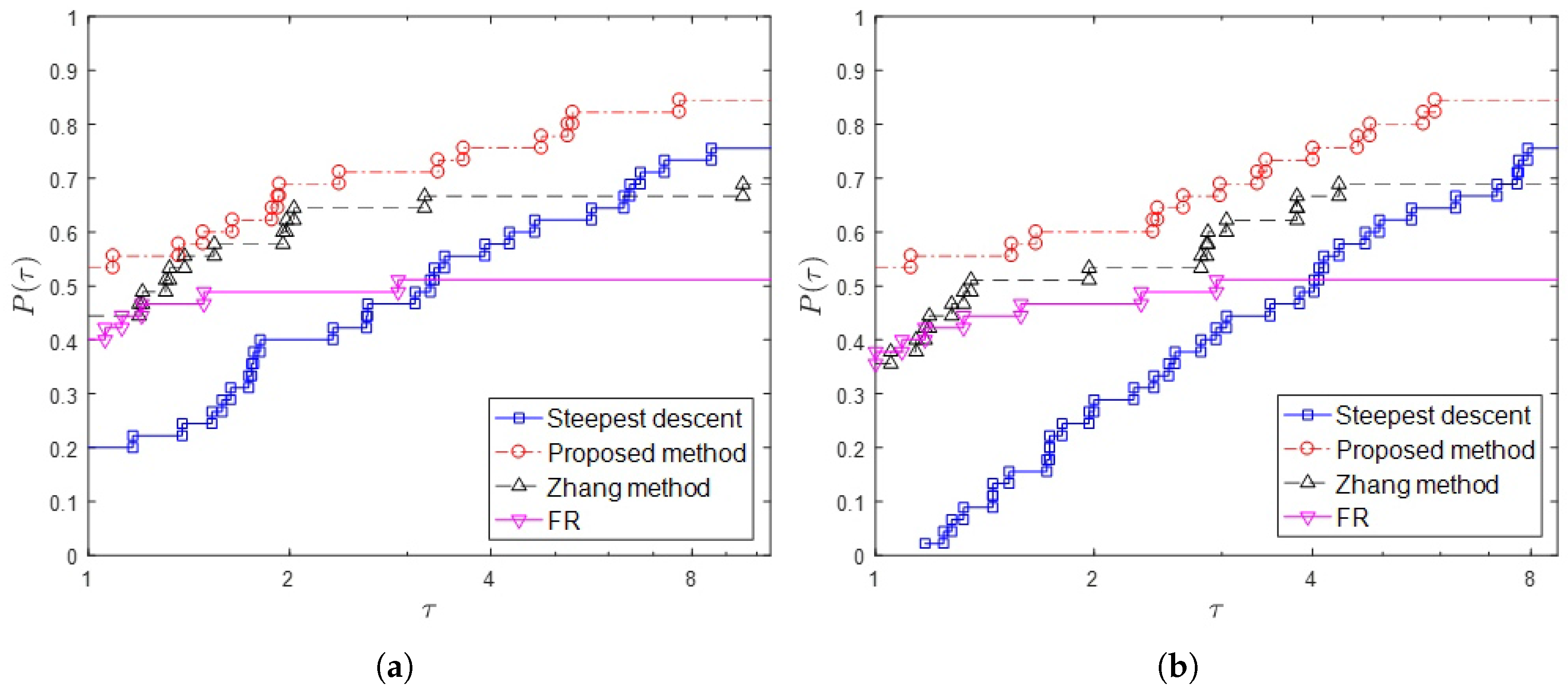
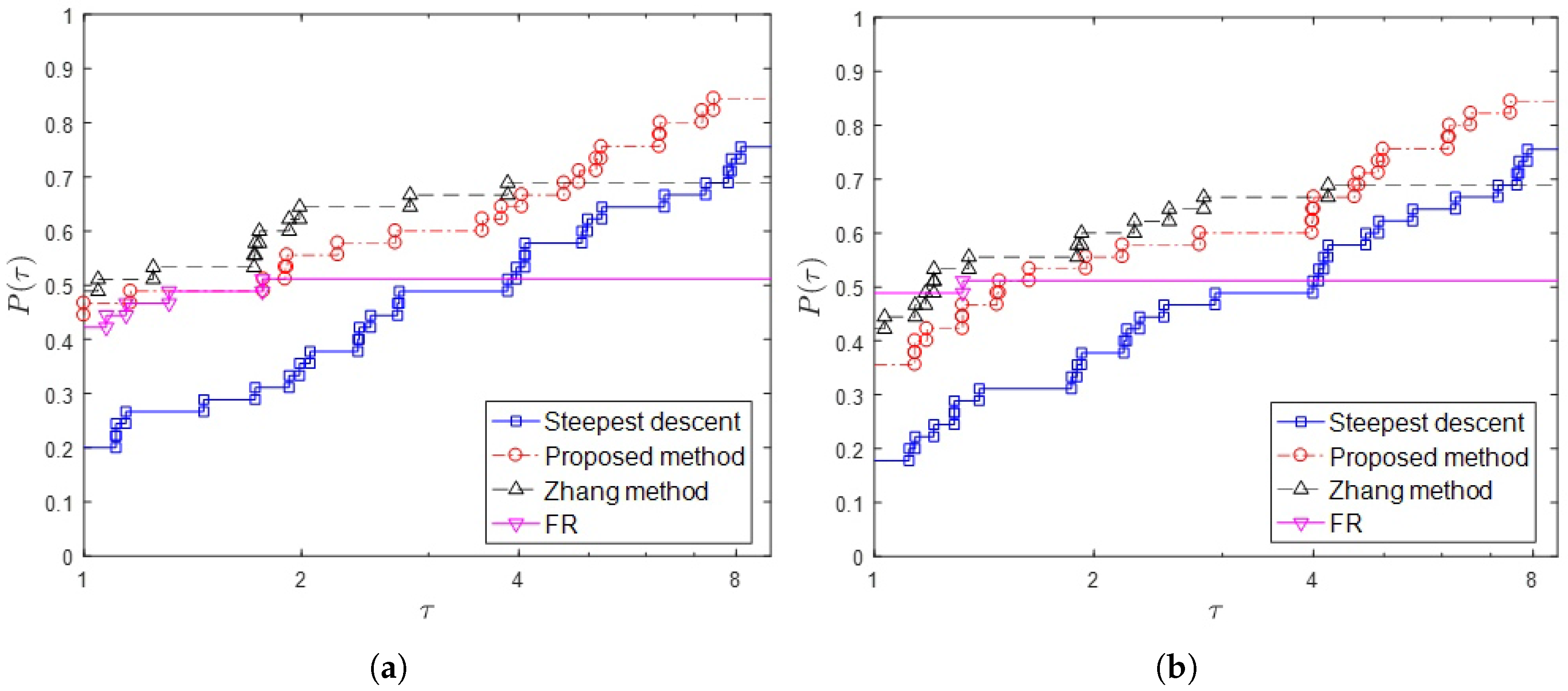
5. Numerical Experiments

In this section, we consider some numerical results for the three-step discretization method. We use MATLAB 2016 (R2016b, MathWorks, Natick, MA, USA). The stopping rule for the Algorithm 1 is designed to decrease the gradient norm to ${10}^{-3}$. Parameters c and $\rho$ are fixed ${10}^{-3}$ and $0.5$, respectively. We set up the parameter ${\alpha }_{initial}=1$ throughout the entire algorithm. The numerical comparisons include:

• Iterative numbers (denote by NI) for attaining the same stopping criterion ${\parallel \nabla f\parallel }_2<{10}^{-3}$.
• Evaluation numbers of f (denote by Nf)
• Evaluation numbers of $\nabla f$ (denote by Ng)
• Difference between the value of the function at the optimal point and the value of the function at the last calculated point as the accuracy of the method; i.e., $error=\parallel f({\mathbf{x}}_{optimal})-f({\mathbf{x}}_{final}){\parallel }_2$ .

We tested 45 problems from the [39,40,41,42].

Table 1. Test problems of general objective functions.

${\mathrm{Function}}^1$	2	Freudenstein and Roth	2	Rosenbrock	2	Powell Badly Scaled	2	Brown Badly Scaled	2
Helical Valley	3	Bard	3	Gaussian	3	Meyer	3	Powell Singular	4
Wood	4	Kowalik and Osborne	4	Brown and Dennis	4	Biggs EXP6	6	Variably Dimensioned	10
${\mathrm{Function}}^{28}$	10	${\mathrm{Function}}^{33}$	10	${\mathrm{Function}}^{34}$	10	Broyden Banded	10	Penalty I	10
Zakharov	10	Qing	10	Extended Rosenbrock	16	Zakharov	40	Alpine N. 1	40
Trigonometric	50	Extended Rosenbrock	100	Extended Powell Singular	100	Penalty I	100	Discrete Integral Equation	100
Broyden Tridiagonal	100	Broyden Banded	100	Zakharov	100	Dixon-Price	100	Penalty I	1000
Rotated Hyper-ellipsoid	1000	Rastrigin	1000	Exponential function	1000	Sum-Squares	1000	Periodic function	1000
Ackley	1000	Griewank	1000	Sphere	1000	Shubert	1000	Quartic	1000

shows function names and their dimension.

In Table 1 ${\mathrm{Function}}^1$ is the following function:

$$f(\mathbf{x},\mathbf{y})=log\left(1-log\left(\mathbf{x}(1-\mathbf{x})\mathbf{y}(1-\mathbf{y})\right)\right).$$

where the optimal solution is ${\mathbf{x}}^{*}=(0.5,0.5)$ and $f({\mathbf{x}}^{*})=1.32776143$ [41] . Also, ${\mathrm{Function}}^{28}$, ${\mathrm{Function}}^{33}$ and ${\mathrm{Function}}^{34}$ are the test functions 28, 33 and 34 in the [42], respectively.

The numerical results of some of the functions in the Table 1 are reported in the following tables.

Table 2. Iteration numbers (NI) for different methods.

Function	Dimension	Steepest Descent	FR	Zhang Method	Proposed Method
${\mathrm{Function}}^1$	2	F	F	F	2
Bard	3	10,381	F	F	3600
Kowalik and Osborne	4	123	F	24	23
Brown and Dennis	4	F	F	90	117
${\mathrm{Function}}^{34}$	10	66	17	66	8
Extended Rosenbrock	16	6504	27	42	663
Zakharov	40	F	F	F	2
Alpine N. 1	40	F	F	F	2
Trigonometric	50	33	F	22	10
Penalty I	100	12	5	28	2
Discrete Integral Equation	100	21	9	21	3
Broyden Banded	100	100	F	F	7
Rotated Hyper-ellipsoid	1000	60	28	24	18
Rastrigin	1000	7	4	28	2
Periodic function	1000	163	8	163	8

shows iterative numbers (NI),

Table 3. The number of function evaluations (Nf) for different methods.

Function	Dimension	Steepest Descent	FR	Zhang Method	Proposed Method
${\mathrm{Function}}^1$	2	F	F	F	9
Bard	3	49,479	F	F	44,354
Kowalik and Osborne	4	360	F	68	152
Brown and Dennis	4	F	F	1468	5521
${\mathrm{Function}}^{34}$	10	1123	283	1123	393
Extended Rosenbrock	16	64,567	232	384	17,876
Zakharov	40	F	F	F	73
Alpine N. 1	40	F	F	F	7
Trigonometric	50	42	F	43	31
Penalty I	100	69	32	84	25
Discrete Integral Equation	100	43	15	43	13
Broyden Banded	100	700	F	F	133
Rotated Hyper-ellipsoid	1000	351	164	163	285
Rastrigin	1000	64	47	29	37
Periodic function	1000	334	23	334	46

compares the Nf,

Table 4. The number of gradient evaluations (Ng) for different methods.

Function	Dimension	Steepest Descent	FR	Zhang Method	Proposed Method
${\mathrm{Function}}^1$	2	F	F	F	7
Bard	3	10,382	F	F	9354
Kowalik and Osborne	4	124	F	25	70
Brown and Dennis	4	F	F	91	352
${\mathrm{Function}}^{34}$	10	67	18	67	25
Extended Rosenbrock	16	6505	28	43	1987
Zakharov	40	F	F	F	7
Alpine N. 1	40	F	F	F	7
Trigonometric	50	34	F	23	31
Penalty I	100	13	6	29	7
Discrete Integral Equation	100	22	10	22	10
Broyden Banded	100	101	F	F	22
Rotated Hyper-ellipsoid	1000	61	29	25	55
Rastrigin	1000	8	5	29	7
Periodic function	1000	164	9	164	25

compares the Ng and

Table 5. Accuracy (error) for different methods.

Function	Dimension	Steepest Descent	FR	Zhang Method	Proposed Method
${\mathrm{Function}}^1$	2	F	F	F	$7.68\times {10}^{-13}$
Bard	3	$7.65\times {10}^{-5}$	F	F	$2.31\times {10}^{-5}$
Kowalik and Osborne	4	$3.70\times {10}^{-5}$	F	$2.18\times {10}^{-6}$	$2.14\times {10}^{-5}$
Brown and Dennis	4	F	F	$1.62\times {10}^{-3}$	$1.62\times {10}^{-3}$
${\mathrm{Function}}^{34}$	10	$2.72\times {10}^{-12}$	$1.05\times {10}^{-12}$	$2.71\times {10}^{-12}$	$8.47\times {10}^{-13}$
Extended Rosenbrock	16	$6.31\times {10}^{-7}$	$9.13\times {10}^{-7}$	$1.92\times {10}^{-10}$	$5.64\times {10}^{-7}$
Zakharov	40	F	F	F	$9.62\times {10}^{-5}$
Alpine N. 1	40	F	F	F	$1.34\times {10}^{-5}$
Trigonometric	50	$1.11\times {10}^{-5}$	F	$2.23\times {10}^{-6}$	$2.56\times {10}^{-5}$
Penalty I	100	$3.50\times {10}^{-7}$	$1.28\times {10}^{-6}$	$5.10\times {10}^{-7}$	$4.10\times {10}^{-7}$
Discrete Integral Equation	100	$1.09\times {10}^{-7}$	$1.59\times {10}^{-7}$	$1.081\times {10}^{-7}$	$7.93\times {10}^{-8}$
Broyden Banded	100	$1.59\times {10}^{-7}$	F	F	$3.42\times {10}^{-9}$
Rotated Hyper-ellipsoid	1000	$1.44\times {10}^{-4}$	$7.19\times {10}^{-5}$	$8.27\times {10}^{-5}$	$1.39\times {10}^{-4}$
Rastrigin	1000	$6.72\times {10}^{-5}$	$1.19\times {10}^{-4}$	$3.87\times {10}^{-4}$	$1.37\times {10}^{-5}$
Periodic function	1000	$6.80\times {10}^{-8}$	$1.12\times {10}^{-9}$	$6.80\times {10}^{-8}$	$1.32\times {10}^{-8}$

presents the error. We compare our method with the steepest descent method, the FR method and the conjugate gradient method in [37] which we refer to as the Zhang method. The letter “F” in the tables shows that the corresponding method did not succeed in approaching the optimal point. The FR method has the most failure modes since it did not produce a descent direction. In comparison with the steepest descent method, the proposed method has fewer iterations and fewer function and gradient evaluations. Also, the proposed method shows good agreement with the conjugate gradient method in [37].

Also, we use the performance profiles in [43] to compare the performance of the considered methods. If the performance profile of a method is higher than the performance profiles of the other methods, then this method performed better than the other methods.

Figure 1a,b and Figure 2a,b show the performance profiles measured in accordance with CPU time, NI, Nf and Ng, respectively. From the viewpoint of CPU time and the number of iterations (NI), we observe in Figure 1 that the three-step discretization method is successful. The proposed method works better than the steepest descent method. Although the FR method is rapid and accurate, it has not led to descent direction in many cases. Therefore, the graph of FR method placed lower than the graph of the steepest descent method for $\tau \ge 4$.

From the viewpoint of the number of function evaluations (Nf) and the number of gradient evaluations (Ng), Figure 2 shows that the Zhang method needs fewer computational costs. In this figure the proposed method almost comparable with the Zhang method. Also, for $\tau \ge 5$ the proposed method is superior to other methods.

6. Conclusions

Based on three-step Taylor expansion and Armijo-line search, we propose the three-step discretization algorithm for unconstrained optimization problems. The presented method uses some information of the objective function which exists in the third-order Taylor series while there is no requirement to calculate higher order derivatives. The global convergence of the proposed algorithm is proved. Some numerical experiments are conducted on the proposed algorithm. In comparison with the steepest descent method, the numerical performance of the proposed method is superior.

References

1. Ahookhosh, M.; Ghaderi, S. On efficiency of nonmonotone Armijo-type line searches. Appl. Math. Model. 2017, 43, 170–190. [Google Scholar] [CrossRef]
2. Andrei, N. A new three-term conjugate gradient algorithm for unconstrained optimization. Numer. Algorithms 2015, 68, 305–321. [Google Scholar] [CrossRef]
3. Edgar, T.F.; Himmelblau, D.M.; Lasdon, L.S. Optimization of Chemical Processes; McGraw-Hill: New York, NY, USA, 2001. [Google Scholar]
4. Nocedal, J.; Wright, S.J. Numerical Optimization; Springer Verlag: New York, NY, USA, 2006. [Google Scholar]
5. Shi, Z.J. Convergence of line search methods for unconstrained optimization. Appl. Math. Comput. 2004, 157, 393–405. [Google Scholar] [CrossRef]
6. Vieira, D.A.G.; Lisboa, A.C. Line search methods with guaranteed asymptotical convergence to an improving local optimum of multimodal functions. Eur. J. Oper. Res. 2014, 235, 38–46. [Google Scholar] [CrossRef]
7. Yuan, G.; Wei, Z.; Lu, X. Global convergence of BFGS and PRP methods under a modified weak Wolfe-Powell line search. Appl. Math. Model. 2017, 47, 811–825. [Google Scholar] [CrossRef]
8. Wang, J.; Zhu, D. Derivative-free restrictively preconditioned conjugate gradient path method without line search technique for solving linear equality constrained optimization. Comput. Math. Appl. 2017, 73, 277–293. [Google Scholar] [CrossRef]
9. Zhou, G. A descent algorithm without line search for unconstrained optimization. Appl. Math. Comput. 2009, 215, 2528–2533. [Google Scholar] [CrossRef]
10. Zhou, G.; Feng, C. The steepest descent algorithm without line search for p-Laplacian. Appl. Math. Comput. 2013, 224, 36–45. [Google Scholar] [CrossRef]
11. Koks, D. Explorations in Mathematical Physics: The Concepts Behind an Elegant Language; Springer Science: New York, NY, USA, 2006. [Google Scholar]
12. Dennis, J.E., Jr.; Schnabel, R.B. Numerical Methods for Unconstrained Optimization and Nonlinear Equations; SIAM: Philadelphia, PA, USA, 1996. [Google Scholar]
13. Otmar, S. A convergence analysis of a method of steepest descent and a two-step algorothm for nonlinear ill–posed problems. Numer. Funct. Anal. Optim. 1996, 17, 197–214. [Google Scholar] [CrossRef]
14. Ebadi, M.J.; Hosseini, A.; Hosseini, M.M. A projection type steepest descent neural network for solving a class of nonsmooth optimization problems. Neurocomputing 2017, 193, 197–202. [Google Scholar] [CrossRef]
15. Yousefpour, R. Combination of steepest descent and BFGS methods for nonconvex nonsmooth optimization. Numer. Algorithms 2016, 72, 57–90. [Google Scholar] [CrossRef]
16. Gonzaga, C.C.; Schneider, R.M. On the steepest descent algorithm for quadratic functions. Comput. Optim. Appl. 2016, 63, 523–542. [Google Scholar] [CrossRef]
17. Jiang, C.B.; Kawahara, M. A three-step finite element method for unsteady incompressible flows. Comput. Mech. 1993, 11, 355–370. [Google Scholar] [CrossRef]
18. Kumar, B.V.R.; Kumar, S. Convergence of Three-Step Taylor Galerkin finite element scheme based monotone schwarz iterative method for singularly perturbed differential-difference equation. Numer. Funct. Anal. Optim. 2015, 36, 1029–1045. [Google Scholar]
19. Kumar, B.V.R.; Mehra, M. A three-step wavelet Galerkin method for parabolic and hyperbolic partial differential equations. Int. J. Comput. Math. 2006, 83, 143–157. [Google Scholar] [CrossRef]
20. Cauchy, A. General method for solving simultaneous equations systems. Comp. Rend. Sci. 1847, 25, 46–89. [Google Scholar]
21. Barzilai, J.; Borwein, J.M. Two-point step size gradient methods. IMA J. Numer. Anal. 1988, 8, 141–148. [Google Scholar] [CrossRef]
22. Dai, Y.H.; Fletcher, R. Projected Barzilai-Borwein methods for large-scale box-constrained quadratic programming. Numer. Math. 2005, 100, 21–47. [Google Scholar]
23. Hassan, M.A.; Leong, W.J.; Farid, M. A new gradient method via quasicauchy relation which guarantees descent. J. Comput. Appl. Math. 2009, 230, 300–305. [Google Scholar] [CrossRef]
24. Leong, W.J.; Hassan, M.A.; Farid, M. A monotone gradient method via weak secant equation for unconstrained optimization. Taiwan. J. Math. 2010, 14, 413–423. [Google Scholar] [CrossRef]
25. Tan, C.; Ma, S.; Dai, Y.; Qian, Y. Barzilai-Borwein step size for stochastic gradient descent. In Proceedings of the 30th Conference on Neural Information Processing Systems, Barcelona, Spain, 5–10 December 2016. [Google Scholar]
26. Raydan, M. On the Barzilai and Borwein choice of steplength for the gradient method. IMA J. Numer. Anal. 1993, 13, 321–326. [Google Scholar] [CrossRef]
27. Dai, Y.H.; Liao, L.Z. R-linear convergence of the Barzilai and Borwein gradient method. IMA J. Numer. Anal. 2002, 26, 1–10. [Google Scholar] [CrossRef]
28. Dai, Y.H. A New Analysis on the Barzilai-Borwein Gradient Method. J. Oper. Res. Soc. China 2013, 1, 187–198. [Google Scholar] [CrossRef]
29. Yuan, Y. A new stepsize for the steepest descent method. J. Comput. Appl. Math. 2006, 24, 149–156. [Google Scholar]
30. Manton, J.M. Modified steepest descent and Newton algorithms for orthogonally constrained optimisation: Part II The complex Grassmann manifold. In Proceedings of the Sixth International Symposium on Signal Processing and its Applications (ISSPA), Kuala Lumpur, Malaysia, 13–16 August 2001. [Google Scholar]
31. Shan, G.H. Gradient-Type Methods for Unconstrained Optimization. Bachelor’s Thesis, University Tunku Abdul Rahman, Petaling Jaya, Malaysia, 2016. [Google Scholar]
32. Hestenes, M.R.; Stiefel, M. Methods of conjugate gradients for solving linear systems. J. Res. Natl. Bur. Stand. 1952, 49, 409–436. [Google Scholar] [CrossRef]
33. Fletcher, R.; Reeves, C.M. Function minimization by conjugate gradients. Comput. J. 1964, 7, 149–154. [Google Scholar] [CrossRef]
34. Hager, W.W.; Zhang, H. A survey of nonlinear conjugate gradient methods. Pac. J. Optim. 2006, 2, 35–58. [Google Scholar]
35. Dai, Y.H.; Liao, L.Z. New conjugacy conditions and related nonlinear conjugate gradient methods. Appl. Math. Optim. 2001, 43, 87–101. [Google Scholar] [CrossRef]
36. Kobayashi, M.; Narushima, M.; Yabe, H. Nonlinear conjugate gradient methods with structured secant condition for nonlinear least squares problems. J. Comput. Appl. Math. 2010, 234, 375–397. [Google Scholar] [CrossRef]
37. Zhang, L.; Zhou, W.; Li, D. Global convergence of a modified Fletcher-Reeves conjugate gradient method with Armijo-type line search. Numer. Math. 2006, 104, 561–572. [Google Scholar] [CrossRef]
38. Sugiki, K.; Narushima, Y.; Yabe, H. Globally convergent three-term conjugate gradient methods that use secant conditions and generate descent search directions for unconstrained optimization. J. Optim. Theory Appl. 2012, 153, 733–757. [Google Scholar] [CrossRef]
39. Jamil, M.; Yang, X.S. A literature survey of benchmark functions for global optimization problems. Int. J. Math. Model. Numer. Optim. 2013, 4, 150–194. [Google Scholar]
40. Molga, M.; Smutnicki, C. Test Functions for Optimization Needs, 2005. Available online: http://www.robertmarks.org/Classes/ENGR5358/Papers/functions.pdf (accessed on 30 June 2013).
41. Papa Quiroz, E.A.; Quispe, E.M.; Oliveira, P.R. Steepest descent method with a generalized Armijo search for quasiconvex functions on Riemannian manifolds. J. Math. Anal. Appl. 2008, 341, 467–477. [Google Scholar] [CrossRef]
42. Moré, J.J.; Garbow, B.S.; Hillstrome, K.E. Testing unconstrained optimization software. ACM Trans. Math. Softw. 1981, 7, 17–41. [Google Scholar]
43. Dolan, E.D.; Moré, J.J. Benchmarking optimization software with performance profiles. Math. Program. Ser. A 2002, 91, 201–213. [Google Scholar]
Figure 1. Performance profiles based on CPU time (a) and the number of iterations (NI) (b) for 45 functions in the Table 1.
Mathematics 06 00063 g001
Figure 2. Performance profiles based on the number of function evaluations (Nf) (a) and the number of gradient evaluations (Ng) (b) for 45 functions in the Table 1.
Mathematics 06 00063 g002