Hypergraphs in m-Polar Fuzzy Environment


Department of Mathematics, University of the Punjab, New Campus, Lahore 54590, Pakistan
*
Author to whom correspondence should be addressed.
Mathematics 2018, 6(2), 28; https://doi.org/10.3390/math6020028
Submission received: 7 February 2018
/
Revised: 15 February 2018
/
Accepted: 16 February 2018
/
Published: 20 February 2018
Abstract
:Fuzzy graph theory is a conceptual framework to study and analyze the units that are intensely or frequently connected in a network. It is used to study the mathematical structures of pairwise relations among objects. An m-polar fuzzy (mF, for short) set is a useful notion in practice, which is used by researchers or modelings on real world problems that sometimes involve multi-agents, multi-attributes, multi-objects, multi-indexes and multi-polar information. In this paper, we apply the concept of mF sets to hypergraphs, and present the notions of regular mF hypergraphs and totally regular mF hypergraphs. We describe the certain properties of regular mF hypergraphs and totally regular mF hypergraphs. We discuss the novel applications of mF hypergraphs in decision-making problems. We also develop efficient algorithms to solve decision-making problems.
1. Introduction
Graph theory has interesting applications in different fields of real life problems to deal with the pairwise relations among the objects. However, this information fails when more than two objects satisfy a certain common property or not. In several real world applications, relationships are more problematic among the objects. Therefore, we take into account the use of hypergraphs to represent the complex relationships among the objects. In case of a set of multiarity relations, hypergraphs are the generalization of graphs, in which a hypergraph may have more than two vertices. Hypergraphs have many applications in different fields including biological science, computer science, declustering problems and discrete mathematics.
In 1994, Zhang [1] proposed the concept of bipolar fuzzy set as a generalization of fuzzy set [2]. In many problems, bipolar information are used, for instance, common efforts and competition, common characteristics and conflict characteristics are the two-sided knowledge. Chen et al. [3] introduced the concept of m-polar fuzzy (mF, for short) set as a generalization of a bipolar fuzzy set and it was shown that 2-polar and bipolar fuzzy set are cryptomorphic mathematical notions. The framework of this theory is that “multipolar information” (unlike the bipolar information which gives two-valued logic) arise because information for a natural world are frequently from n factors . For example, ‘Pakistan is a good country’. The truth value of this statement may not be a real number in . Being a good country may have several properties: good in agriculture, good in political awareness, good in regaining macroeconomic stability etc. Each component may be a real number in . If n is the number of such components under consideration, then the truth value of the fuzzy statement is a n-tuple of real numbers in , that is, an element of . The perception of fuzzy graphs based on Zadeh’s fuzzy relations [4] was introduced by Kauffmann [5]. Rosenfeld [6] described the fuzzy graphs structure. Later, some remarks were given by Bhattacharya [7] on fuzzy graphs. Several concepts on fuzzy graphs were introduced by Mordeson and Nair [8]. In 2011, Akram introduced the notion of bipolar fuzzy graphs in [9]. Li et al. [10] considered different algebraic operations on mF graphs.
In 1977, Kauffmann [5] proposed the fuzzy hypergraphs. Chen [11] studied the interval-valued fuzzy hypergraph. Generalization and redefinition of the fuzzy hypergraph were explained by Lee-Kwang and Keon-Myung [12]. Parvathi et al. [13] introduced the concept of intuitionistic fuzzy hypergraphs. Samanta and Pal [14] dealt with bipolar fuzzy hypergraphs. Later on, Akram et al. [15] considered certain properties of the bipolar fuzzy hypergraph. Bipolar neutrosophic hypergraphs with applications were presented by Akram and Luqman [16]. Sometimes information is multipolar, that is, a communication channel may have various signal strengths from the others due to various reasons including atmosphere, device distribution, mutual interference of satellites etc. The accidental mixing of various chemical substances could cause toxic gases, fire or explosion of different degrees. All these are components of multipolar knowledge which are fuzzy in nature. This idea motivated researchers to study mF hypergraphs [17]. Akram and Sarwar [18] considered transversals of mF hypergraphs with applications. In this research paper, we introduce the idea of regular and totally regular mF hypergraphs and investigate some of their properties. We discuss the new applications of mF hypergraphs in decision-making problems. We develop efficient algorithms to solve decision-making problems and compute the time complexity of algorithms. For other notations, terminologies and applications not mentioned in the paper, the readers are referred to [19,20,21,22,23,24,25,26,27,28,29,30,31].
In this paper, we will use the notations defined in Table 1.
2. Notions of mF Hypergraph
Definition 1.
An mF set on a non-empty crisp set X is a function . The degree of each element is denoted by , where is the i-th projection mapping [3].
Note that (m-th-power of ) is considered as a poset with the point-wise order where m is an arbitrary ordinal number (we make an appointment that when ), ≤ is defined by for each , and is the i-th projection mapping . is the greatest value and is the smallest value in .
Definition 2.
Let A be an mF subset of a non-empty fuzzy subset of a non-empty set X. An mF relation on A is an mF subset B of defined by the mapping such that for all
, where denotes the i-th degree of membership of a vertex x and denotes the i-th degree of membership of the edge .
Definition 3.
An mF graph is a pair , where is an mF set in X and is an mF relation on X such that
, for all and for all for all . A is called the mF vertex set of G and B is called the mF edge set of G, respectively [3].
Definition 4.
An mF hypergraph on a non-empty set X is a pair [17], where is a family of mF subsets on X and B is an mF relation on the mF subsets such that
- 1.
- for all .
- 2.
- , for all .
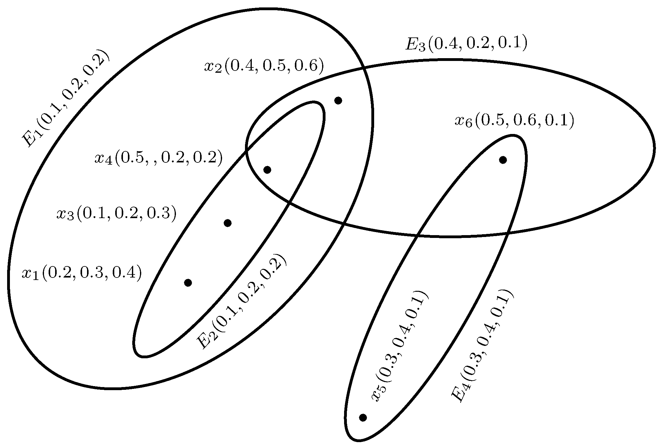
Example 1.
Example 2.
Definition 5.
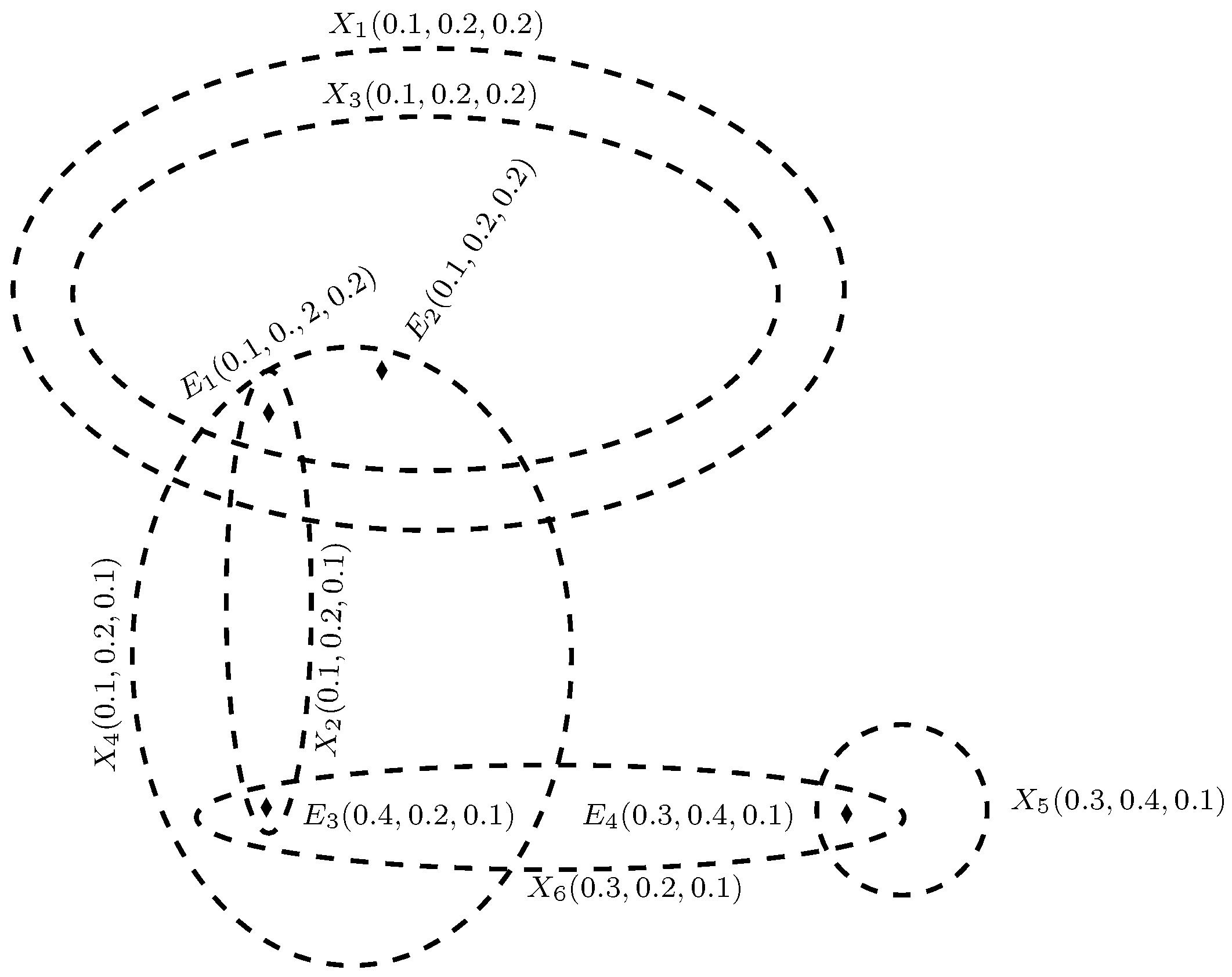
Let be an mF hypergraph on a non-empty set X [17]. The dual mF hypergraph of H, denoted by , is defined as
- 1.
- is the mF set of vertices of .
- 2.
- If then, is an mF set on the family of hyperedges such that, ={ is a hyperedge of H}, i.e., is the mF set of those hyperedges which share the common vertex and .
Example 3.
Definition 6.
The open neighourhood of a vertex x in the mF hypergraph is the set of adjacent vertices of x excluding that vertex and it is denoted by .
Example 4.
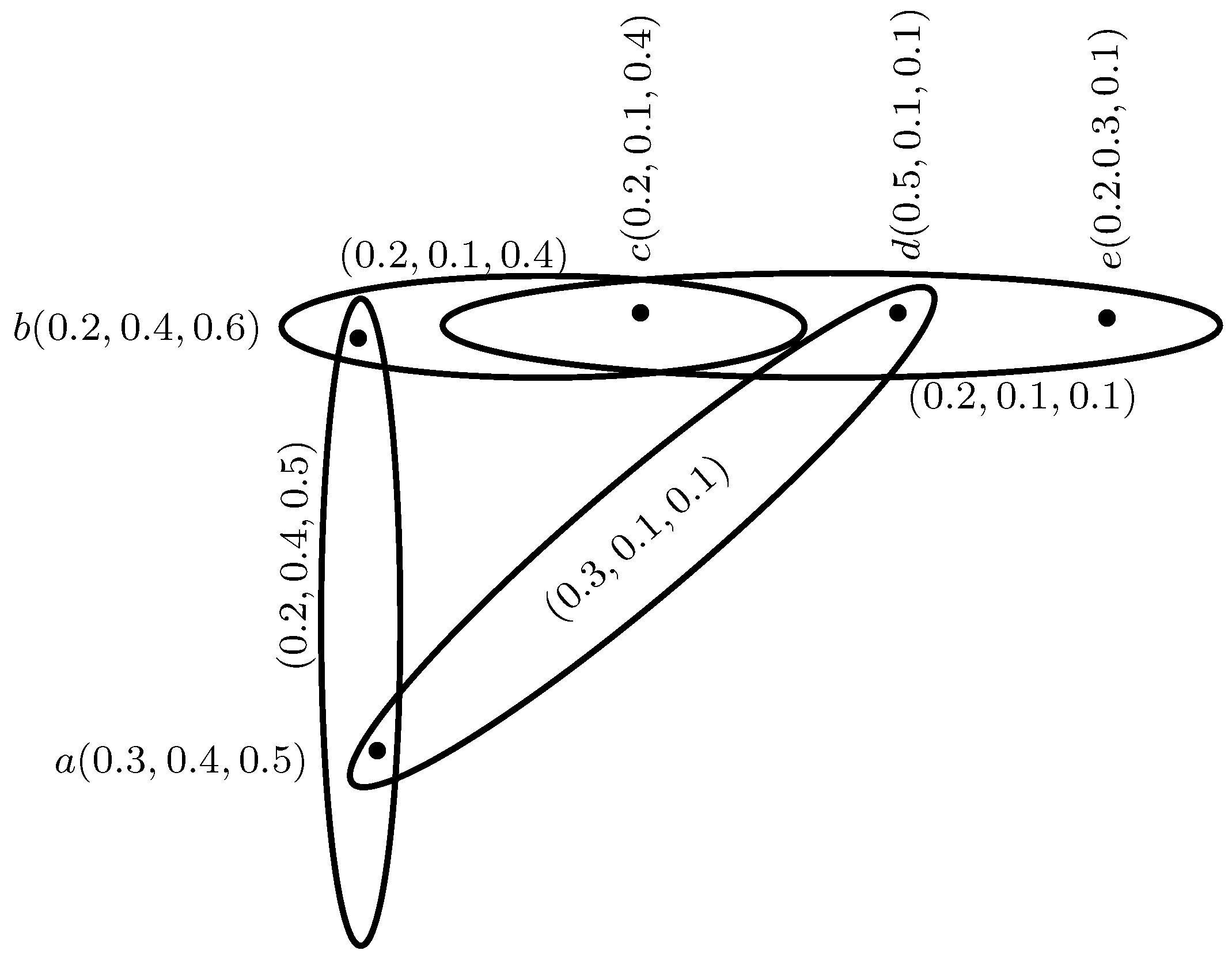
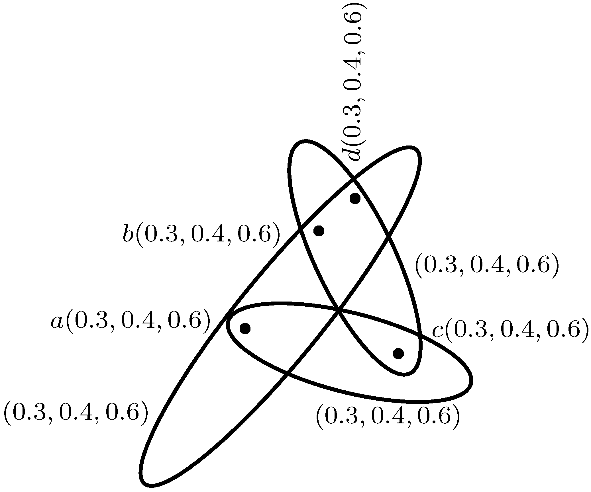
Consider the 3-polar fuzzy hypergraph , where is a family of 3-polar fuzzy subsets on and B is a 3-polar fuzzy relation on the 3-polar fuzzy subsets , where , , , . In this example, open neighourhood of the vertex a is b and d, as shown in Figure 5.
Definition 7.
The closed neighourhood of a vertex x in the mF hypergraph is the set of adjacent vertices of x including that vertex and it is denoted by .
Example 5.
Consider the 3-polar fuzzy hypergraph , where is a family of 3-polar fuzzy subsets on and B is a 3-polar fuzzy relation on the 3-polar fuzzy subsets , where , , , . In this example, closed neighourhood of the vertex a is a, b and d, as shown in Figure 5.
Definition 8.
Let be an mF hypergraph on crisp hypergraph . If all vertices in A have the same open neighbourhood degree n, then H is called n-regular mF hypergraph.
Definition 9.
The open neighbourhood degree of a vertex x in H is denoted by and defined by ), where
Example 6.
Consider the 3-polar fuzzy hypergraph , where is a family of 3-polar fuzzy subsets on and B is a 3-polar fuzzy relation on the 3-polar fuzzy subsets , where , , , . The open neighbourhood degree of a vertex a is .
Definition 10.
Let be an mF hypergraph on crisp hypergraph . If all vertices in A have the same closed neighbourhood degree m, then H is called m-totally regular mF hypergraph.
Definition 11.
The closed neighbourhood degree of a vertex x in H is denoted by and defined by where
Example 7.
Consider the 3-polar fuzzy hypergraph , where is a family of 3-polar fuzzy subsets on and B is a 3-polar fuzzy relation on the 3-polar fuzzy subsets , where , , , . The closed neighbourhood degree of a vertex a is .
Example 8.
Consider the 3-polar fuzzy hypergraph , where is a family of 3-polar fuzzy subsets on and B is a 3-polar fuzzy relation on the 3-polar fuzzy subsets , where
By routine calculations, we can show that the above 3-polar fuzzy hypergraph is neither regular nor totally regular.
Example 9.
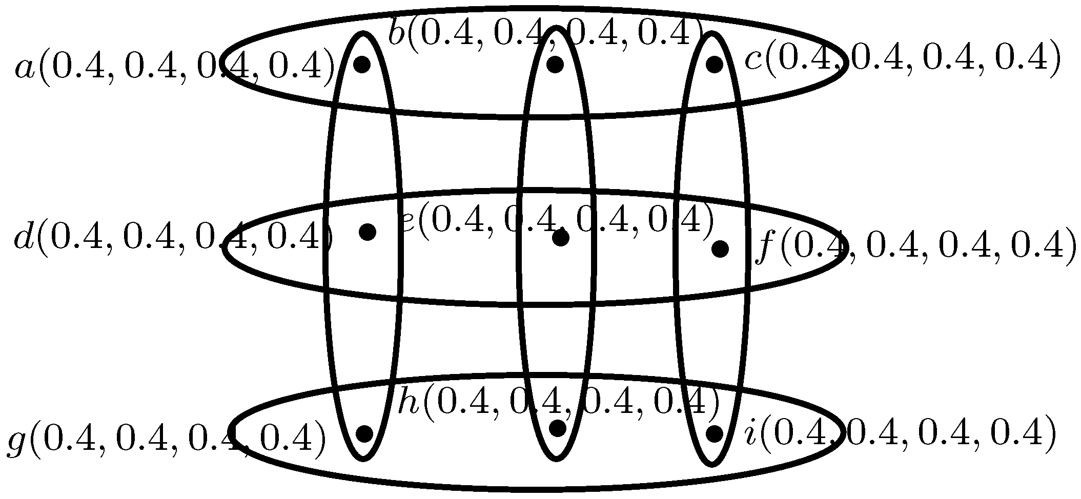
Consider the 4-polar fuzzy hypergraph ; define and , where
By routine calculations, we see that the 4-polar fuzzy hypergraph as shown in Figure 6 is both regular and totally regular.
Remark 1.
- 1.
- For an mF hypergraph to be both regular and totally regular, the number of vertices in each hyperedge must be the same. Suppose that for every j, then H is said to be k-uniform.
- 2.
- Each vertex lies in exactly the same number of hyperedges.
Definition 12.
Let be a regular mF hypergraph. The order of a regular fuzzy hypergraph H is
for every . The size of a regular mF hypergraph is , where
Example 10.
Consider the 4-polar fuzzy hypergraph ; define and , where
The order of H is, and
We state the following propositions without proof.
Proposition 1.
The size of a n-regular mF hypergraph is ,
Proposition 2.
If H is both n-regular and m-totally regular mF hypergraph , then , where
Proposition 3.
If H is both m-totally regular mF hypergraph , then
Theorem 1.
Let be an mF hypergraph of a crisp hypergraph . Then is a constant function if and only if the following are equivalent:
- (a)
- H is a regular mF hypergraph,
- (b)
- H is a totally regular mF hypergraph.
Proof.
Suppose that , where is a constant function. That is, for all , .
: Suppose that H is n-regular mF hypergraph. Then , for all . By using definition 11, for all . Hence, H is a totally regular mF hypergraph.
: Suppose that H is a m-totally regular mF hypergraph. Then , for all ,
Thus, H is a regular mF hypergraph. Hence (1) and (2) are equivalent.
Conversely, suppose that (1) and (2) are equivalent, i.e. H is regular if and only if H is totally regular. On contrary, suppose that A is not constant, that is, for some x and y in A. Let be a n-regular mF hypergraph; then
Consider,
Since and are not equal for some x and y in X, hence and are not equal, thus H is not a totally regular m-poalr fuzzy hypergraph, which is again a contradiction to our assumption.
Next, let H be a totally regulr mF hypergraph, then .
That is,
Since the right hand side of the above equation is nonzero, the left hand side of the above equation is also nonzero. Thus and are not equal, so H is not a regular mF hypergraph, which is again contradiction to our assumption. Hence, A must be constant and this completes the proof. ☐
Theorem 2.
If an mF hypergraph is both regular and totally regular, then is constant function.
Proof.
Let H be a regular and totally regular mF hypergraph. Then
and
Hence, is a constant function. ☐
Remark 2.
The converse of Theorem 1 may not be true, in general. Consider a 3-polar fuzzy hypergraph , define ,
Then , where is a constant function. But . Also . So H is neither regular nor totally regular mF hypergraph.
Definition 13.
An mF hypergraph is called complete if for every that is, contains all the remaining vertices of X except x.
Example 11.
Consider a 3-polar fuzzy hypergraph as shown in Figure 7, where and , where , , . Then , ,
Remark 3.
For a complete mF hypergraph, the cardinality of is the same for every vertex.
Theorem 3.
Every complete mF hyprgraph is a totally regular mF hypergraph.
Proof.
Since given mF hypergraph H is complete, each vertex lies in exactly the same number of hyperedges and each vertex has the same closed neighborhood degree m. That is, for all Hence H is m-totally regular. ☐
3. Applications to Decision-Making Problems
Analysis of human nature and its culture has been entangled with the assessment of social networks for many years. Such networks are refined by designating one or more relations on the set of individuals and the relations can be taken from efficacious relationships, facets of some management and from a large range of others means. For super-dyadic relationships between the nodes, network models represented by simple graph are not sufficient. Natural presence of hyperedges can be found in co-citation, e-mail networks, co-authorship, web log networks and social networks etc. Representation of these models as hypergraphs maintain the dyadic relationships.
3.1. Super-Dyadic Managements in Marketing Channels
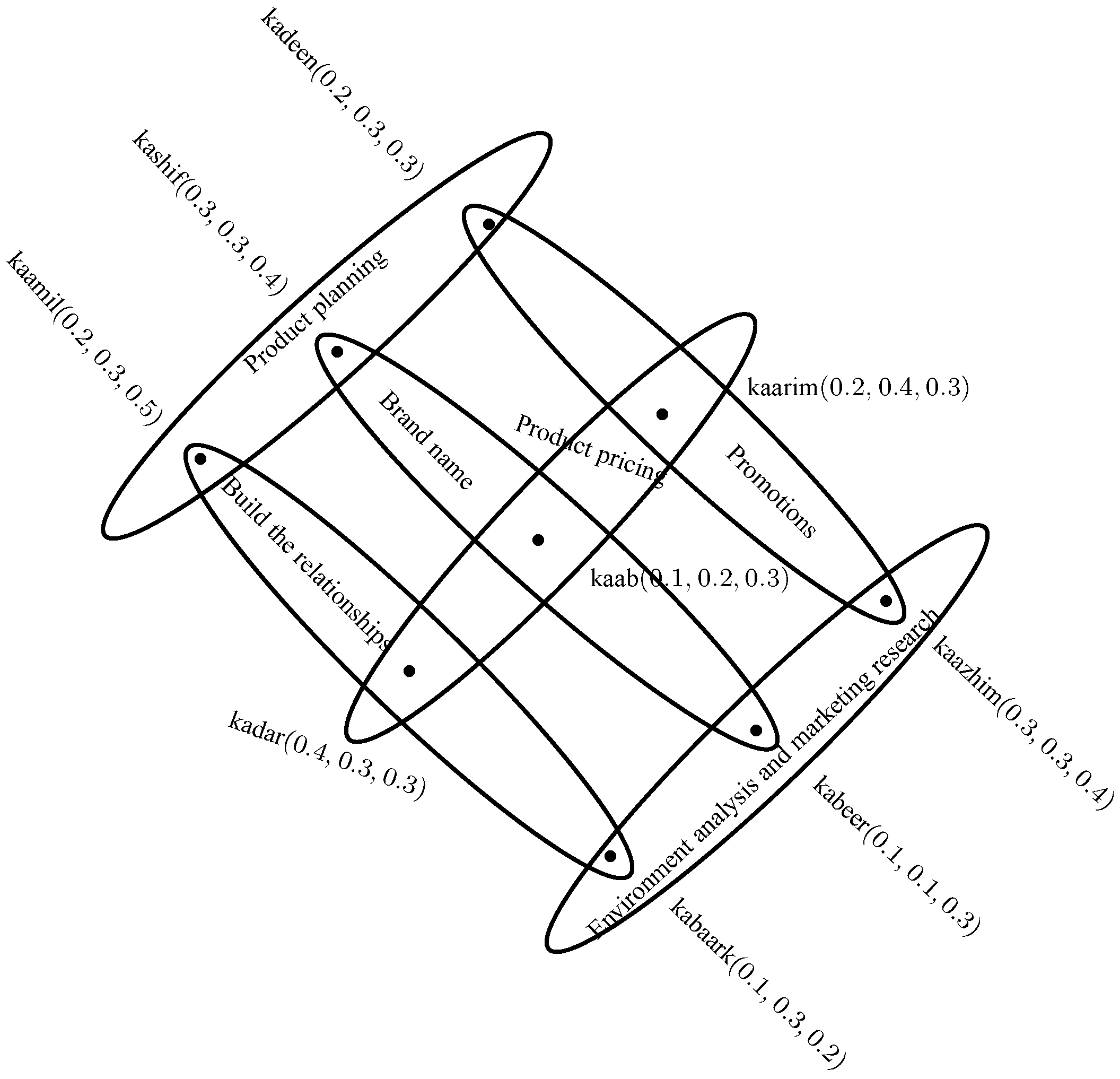
In marketing channels, dyadic correspondence organization has been a basic implementation. Marketing researchers and managers have realized that their common engagement in marketing channels is a central key for successful marketing and to yield benefits for the company. mF hypergraphs consist of marketing managers as vertices and hyperedges show their dyadic communication involving their parallel thoughts, objectives, plans, and proposals. The more powerful close relation in the research is more beneficial for the marketing strategies and the production of an organization. A 3-polar fuzzy network model showing the dyadic communications among the marketing managers of an organization is given in Figure 8.
The membership degrees of each person symbolize the percentage of its dyadic behaviour towards the other people of the same dyad group. The adjacent level between any pair of vertices illustrates how proficient their dyadic relationship is. The adjacent levels are given in Table 4.
It can be seen that the most capable dyadic pair is (Kashif, Kaamil). 3-polar fuzzy hyperedges are taken as different digital marketing strategies adopted by the different dyadic groups of the same organization. The vital goal of this model is to determine the most potent dyad of digital marketing techniques. The six different groups are made by the marketing managers and the digital marketing strategies adopted by these six groups are represented by hyperedges. i.e., the 3-polar fuzzy hyperedges show the following strategies {Product pricing, Product planning, Environment analysis and marketing research, Brand name, Build the relationships, Promotions}, respectively. The exclusive effects of membership degrees of each marketing strategy towards the achievements of an organization are given in Table 5.
Effective dyads of market strategies enhance the performance of an organization and discover the better techniques to be adopted. The adjacency of all dyadic communication managements is given in Table 6.
The most dominant and capable marketing strategies adopted mutually are Product planning and Promotions. Thus, to increase the efficiency of an organization, dyadic managements should make powerful planning for products and use the promotions skill to attract customers to purchase their products. The membership degrees of this dyad is (0.2, 0.3, 0.3) which shows that the amalgamated effect of this dyad will increase the profitable growth of an organization up to 20%, instruction manual for company success up to 30%, create longevity of the business up to 30% . Thus, to promote the performance of an organization, super dyad marketing communications are more energetic. The method of determining the most effective dyads is explained in the following algorithm.
| Algorithm 1 |
|
3.2. m-Polar Fuzzy Hypergraphs in Work Allotment Problem
In customer care centers, availability of employees plays a vital role in solving customer problems. Such a department should ensure that the system has been managed carefully to overcome practical difficulties. A lot of customers visit such centers to find a solution of their problems. In this part, focus is given to alteration of duties for the employees taking leave. The problem is that employees are taking leave without proper intimation and alteration. We now show the importance of m-polar fuzzy hypergraphs for the allocation of duties to avoid any difficulties.
Consider the example of a customer care center consisting of 30 employees. Assuming that six workers are necessary to be available at their duties. We present the employees as vertices and the degree of membership of each employee represents the work load, percentage of available time and number of workers who are also aware of the employee’s work type. The range of values for present time and the workers, knowing the type of work is given in Table 7 and Table 8.
The degree of membership of each edge represents the common work load, percentage of available time and number of workers who are also aware of the employee’s work type. This phenomenon can be represented by a 3-polar fuzzy graph as shown in Figure 9.
Using Algorithm 2, the strength of allocation and alteration of duties among employees is given in Table 9.
Column 3 in Table 9 shows the percentage of alteration of duties. For example, in case of leave, duties of can be given to and similarly for other employees.
The method for the calculation of alteration of duties is given in Algorithm 2.
| Algorithm 2 |
|
3.3. Availability of Books in Library
A library in a college is a collection of sources of information and similar resources, made accessible to the student community for reference and examination preparation. A student preparing for a given examination will use the knowledge sources such as
- Prescribed textbooks (A)
- Reference books in syllabus (B)
- Other books from library (C)
- Knowledgeable study materials (D)
- E-gadgets and internet (E)
It is important to consider the maximum availability of the sources which students mostly use. This phenomenon can be discussed using polar fuzzy hypergraphs. We now calculate the importance of each source in the student community.
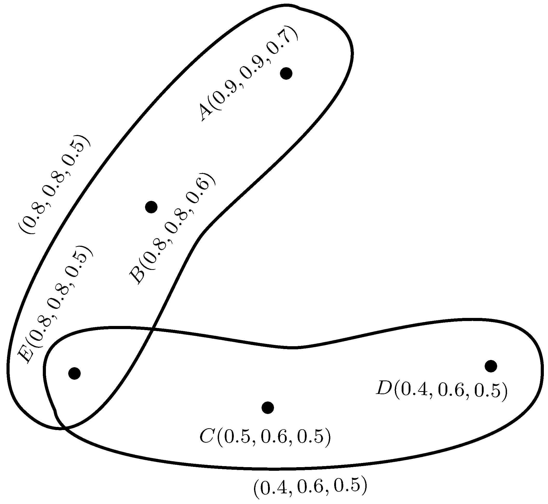
Consider the example of five library resources in a college. We represent these sources as vertices in a polar fuzzy hypergraph. The degree of membership of each vertex represents the percentage of students using a particular source for exam preparation, percentage of faculty members using the sources and number of sources available. The degree of membership of each edge represents the common percentage. The polar fuzzy hypergraph is shown in Figure 10.
Using Algorithm 3, the strength of each library source in given in Table 10.
Column 3 in Table 10 shows that sources A and B are mostly used by students and faculty. Therefore, these should be available in maximum number. There is also a need to confirm the availability of source E to students and faculty.
The method for the calculation of percentage importance of the sources is given in Algorithm 3 whose net time complexity is O.
| Algorithm 3 |
|
4. Conclusions
Hypergraphs are generalizations of graphs. Many problems which cannot be handled by graphs can be solved using hypergraphs. mF graph theory has numerous applications in various fields of science and technology including artificial intelligence, operations research and decision making. An mF hypergraph constitutes a generalization of the notion of an mF fuzzy graph. mF hypergraphs play an important role in discussing multipolar uncertainty among several individuals. In this research article, we have conferred certain concepts of regular mF hypergraphs and applications of mF hypergraphs in decision-making problems. We aim to generalize our notions to (1) mF soft hypergraphs, (2) soft rough mF hypergraphs, (3) soft rough hypergraphs, and (4) intuitionistic fuzzy rough hypergraphs.
Author Contributions
Muhammad Akram and Gulfam Shahzadi conceived and designed the experiments; Muhammad Akram performed the experiments; Muhammad Akram and Gulfam Shahzadi analyzed the data; Gulfam Shahzadi wrote the paper.
Conflicts of Interest
The authors declare no conflict of interest regarding the publication of this research article.
References
- Zhang, W.R. Bipolar fuzzy sets and relations: a computational framework forcognitive modeling and multiagent decision analysis. In Proceedings of the Fuzzy Information Processing Society Biannual Conference, Industrial Fuzzy Control and Intelligent Systems Conference and the NASA Joint Technology Workshop on Neural Networks and Fuzzy Logic, San Antonio, TX, USA, 18–21 December 1994; pp. 305–309. [Google Scholar] [CrossRef]
- Zadeh, L.A. Fuzzy sets. Inf. Control 1965, 8, 338–353. [Google Scholar] [CrossRef]
- Chen, J.; Li, S.; Ma, S.; Wang, X. m-Polar fuzzy sets: An extension of bipolar fuzzy sets. Sci. World J. 2014, 8. [Google Scholar] [CrossRef] [PubMed]
- Zadeh, L.A. Similarity relations and fuzzy orderings. Inf. Sci. 1971, 3, 177–200. [Google Scholar] [CrossRef]
- Kaufmann, A. Introduction la Thorie des Sous-Ensembles Flous Lusage des Ingnieurs (Fuzzy Sets Theory); Masson: Paris, French, 1973. [Google Scholar]
- Rosenfeld, A. Fuzzy Graphs, Fuzzy Sets and Their Applications; Academic Press: New York, NY, USA, 1975; pp. 77–95. [Google Scholar]
- Bhattacharya, P. Remark on fuzzy graphs. Pattern Recognit. Lett. 1987, 6, 297–302. [Google Scholar] [CrossRef]
- Mordeson, J.N.; Nair, P.S. Fuzzy graphs and fuzzy hypergraphs. In Studies in Fuzziness and Soft Computing; Springer-Verlag: Berlin Heidelberg, Germany, 2000. [Google Scholar]
- Akram, M. Bipolar fuzzy graphs. Inf. Sci. 2011, 181, 5548–5564. [Google Scholar] [CrossRef]
- Li, S.; Yang, X.; Li, H.; Ma, M. Operations and decompositions of m-polar fuzzy graphs. Basic Sci. J. Text. Univ. 2017, 30, 149–162. [Google Scholar]
- Chen, S.M. Interval-valued fuzzy hypergraph and fuzzy partition. IEEE Trans. Syst. Man Cybern. B Cybern. 1997, 27, 725–733. [Google Scholar] [CrossRef] [PubMed]
- Lee-Kwang, H.; Lee, K.M. Fuzzy hypergraph and fuzzy partition. IEEE Trans. Syst. Man Cybern. 1995, 25, 196–201. [Google Scholar] [CrossRef]
- Parvathi, R.; Thilagavathi, S.; Karunambigai, M.G. Intuitionistic fuzzy hypergraphs. Cybern. Inf. Technol. 2009, 9, 46–48. [Google Scholar]
- Samamta, S.; Pal, M. Bipolar fuzzy hypergraphs. Int. J. Fuzzy Log. Intell. Syst. 2012, 2, 17–28. [Google Scholar] [CrossRef]
- Akram, M.; Dudek, W.A.; Sarwa, S. Properties of bipolar fuzzy hypergraphs. Ital. J. Pure Appl. Math. 2013, 31, 141–160. [Google Scholar]
- Akram, M.; Luqman, A. Bipolar neutrosophic hypergraphs with applications. J. Intell. Fuzzy Syst. 2017, 33, 1699–1713. [Google Scholar] [CrossRef]
- Akram, M.; Sarwar, M. Novel application of m-polar fuzzy hypergraphs. J. Intell. Fuzzy Syst. 2017, 32, 2747–2762. [Google Scholar] [CrossRef]
- Akram, M.; Sarwar, M. Transversals of m-polar fuzzy hypergraphs with applications. J. Intell. Fuzzy Syst. 2017, 33, 351–364. [Google Scholar] [CrossRef]
- Akram, M.; Adeel, M. mF labeling graphs with application. Math. Comput. Sci. 2016, 10, 387–402. [Google Scholar] [CrossRef]
- Akram, M.; Waseem, N. Certain metrics in m-polar fuzzy graphs. N. Math. Nat. Comput. 2016, 12, 135–155. [Google Scholar] [CrossRef]
- Akram, M.; Younas, H.R. Certain types of irregular m-polar fuzzy graphs. J. Appl. Math. Comput. 2017, 53, 365–382. [Google Scholar] [CrossRef]
- Akram, M.; Sarwar, M. Novel applications of m-polar fuzzy competition graphs in decision support system. Neural Comput. Appl. 2017, 1–21. [Google Scholar] [CrossRef]
- Chen, S.M. A fuzzy reasoning approach for rule-based systems based on fuzzy logics. IEEE Trans. Syst. Man Cybern. B Cybern. 1996, 26, 769–778. [Google Scholar] [CrossRef] [PubMed]
- Chen, S.M.; Lin, T.E.; Lee, L.W. Group decision making using incomplete fuzzy preference relations based on the additive consistency and the order consistency. Inf. Sci. 2014, 259, 1–15. [Google Scholar] [CrossRef]
- Chen, S.M.; Lee, S.H.; Lee, C.H. A new method for generating fuzzy rules from numerical data for handling classification problems. Appl. Artif. Intell. 2001, 15, 645–664. [Google Scholar] [CrossRef]
- Horng, Y.J.; Chen, S.M.; Chang, Y.C.; Lee, C.H. A new method for fuzzy information retrieval based on fuzzy hierarchical clustering and fuzzy inference techniques. IEEE Trans. Fuzzy Syst. 2005, 13, 216–228. [Google Scholar] [CrossRef]
- Narayanamoorthy, S.; Tamilselvi, A.; Karthick, P.; Kalyani, S.; Maheswari, S. Regular and totally regular fuzzy hypergraphs. Appl. Math. Sci. 2014, 8, 1933–1940. [Google Scholar] [CrossRef]
- Radhamani, C.; Radhika, C. Isomorphism on fuzzy hypergraphs. IOSR J. Math. 2012, 2, 24–31. [Google Scholar]
- Sarwar, M.; Akram, M. Certain algorithms for computing strength of competition in bipolar fuzzy graphs. Int. J. Uncertain. Fuzz. 2017, 25, 877–896. [Google Scholar] [CrossRef]
- Sarwar, M.; Akram, M. Representation of graphs using m-polar fuzzy environment. Ital. J. Pure Appl. Math. 2017, 38, 291–312. [Google Scholar]
- Sarwar, M.; Akram, M. Novel applications of m-polar fuzzy concept lattice. N. Math. Nat. Comput. 2017, 13, 261–287. [Google Scholar] [CrossRef]
Figure 1.
4-Polar fuzzy hypergraph.
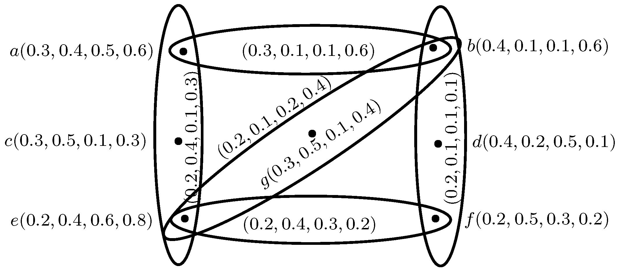
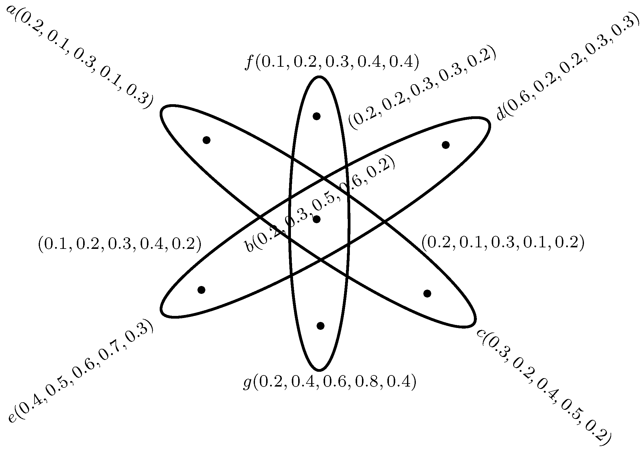
Figure 2.
5-Polar fuzzy hypergraph.

Figure 3.
3-Polar fuzzy hypergraph.

Figure 4.
Dual 3-polar fuzzy hypergraph.

Figure 5.
3-Polar fuzzy hypergraph.

Figure 6.
4-Polar regular and totally regular fuzzy hypergraph.

Figure 7.
3-Polar fuzzy hypergraph.

Figure 8.
Super-dyadic managements in marketing channels.

Figure 9.
3-Polar fuzzy graph.
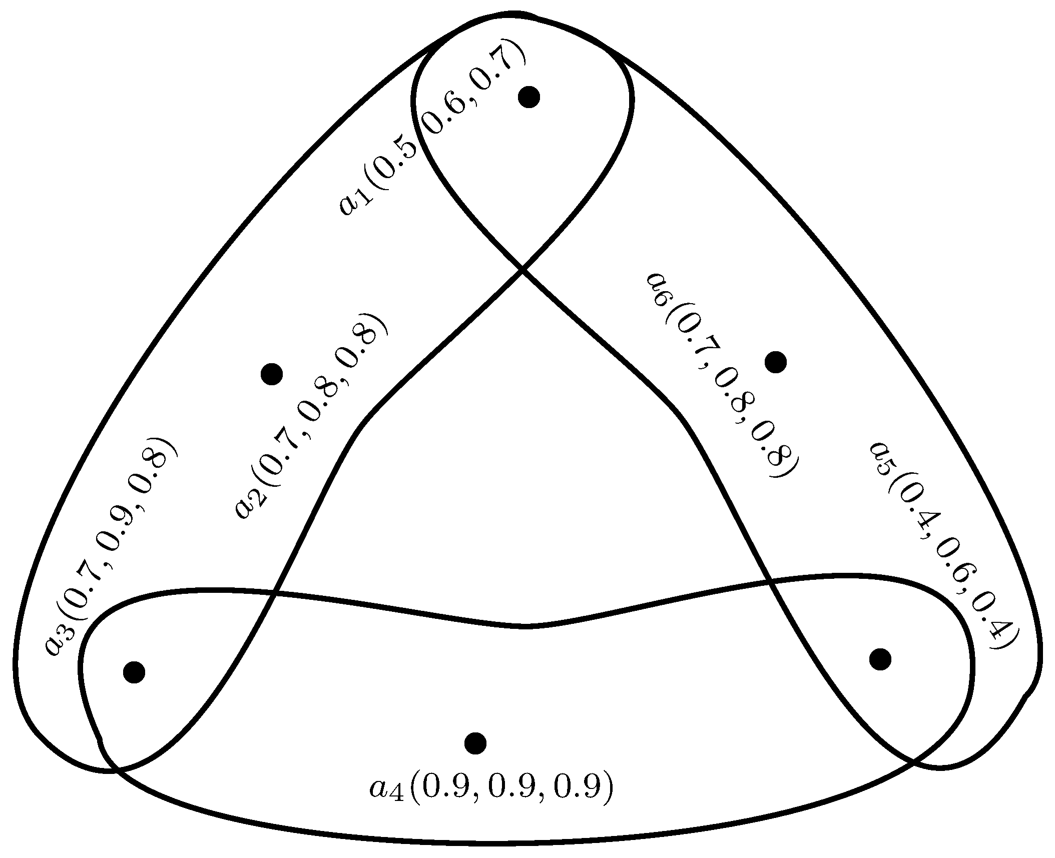
Figure 10.
3-Polar fuzzy hypergraph.

Table 1.
Notations.
| Symbol | Definition |
|---|---|
| Crisp hypergraph | |
| mF hypergraph | |
| Dual mF hypergraph | |
| Open neighourhood degree of a vertex in H | |
| Closed neighourhood degree of a vertex in H | |
| Adjacent level of two vertices | |
| Adjacent level of two hyperedges |
Table 2.
4-polar fuzzy subsets.
| a | (0.3,0.4,0.5,0.6) | (0,0,0,0) | (0.3,0.4,0.5,0.6) | (0,0,0,0) | (0,0,0,0) |
| b | (0,0,0,0) | (0.4,0.1,0.1,0.6) | (0.4,0.1,0.1,0.6) | (0,0,0,0) | (0.4,0.1,0.1,0.6) |
| c | (0.3,0.5,0.1,0.3) | (0,0,0,0) | (0,0,0,0) | (0,0,0,0) | (0,0,0,0) |
| d | (0,0,0,0) | (0.4,0.2,0.5,0.1) | (0,0,0,0) | (0,0,0,0) | (0,0,0,0) |
| e | (0.2,0.4,0.6,0.8) | (0,0,0,0) | (0,0,0,0) | (0.2,0.4,0.6,0.8) | (0.2,0.4,0.6,0.8) |
| f | (0,0,0,0) | (0.2,0.5,0.3,0.2) | (0,0,0,0) | (0.2,0.5,0.3,0.2) | (0,0,0,0) |
| g | (0,0,0,0) | (0,0,0,0) | (0,0,0,0) | (0,0,0,0) | (0.3,0.5,0.1,0.4) |
Table 3.
5-polar fuzzy subsets.
| a | (0.2,0.1,0.3,0.1,0.3) | (0,0,0,0,0) | (0,0,0,0,0) |
| b | (0.2,0.3,0.5,0.6,0.2) | (0.2,0.3,0.5,0.6,0.2) | (0.2,0.3,0.5,0.6,0.2) |
| c | (0.3,0.2,0.4,0.5,0.2) | (0,0,0,0,0) | (0,0,0,0,0) |
| d | (0,0,0,0,0) | (0.6,0.2,0.2,0.3,0.3) | (0,0,0,0,0) |
| e | (0,0,0,0,0) | (0.4,0.5,0.6,0.7,0.3) | (0,0,0,0,0) |
| f | (0,0,0,0,0) | (0,0,0,0,0) | (0.1,0.2,0.3,0.4,0.4) |
| g | (0,0,0,0,0) | (0,0,0,0,0) | (0.2,0.4,0.6,0.8,0.4) |
Table 4.
Adjacent levels.
| Dyad pairs | Adjacent level | Dyad pairs | Adjacent level |
|---|---|---|---|
| (Kadeen, Kashif) | (0.2,0.3,0.3) | (Kaarim, Kaazhim) | (0.2,0.3,0.3) |
| (Kadeen, Kaamil) | (0.2,0.3,0.3) | (Kaarim, Kaab) | (0.1,0.2,0.3) |
| (Kadeen, Kaarim) | (0.2,0.3,0.3) | (Kaarim, Kadar) | (0.2,0.3,0.3) |
| (Kadeen, Kaazhim) | (0.2,0.3,0.3) | (Kaab, Kadar) | (0.1,0.2,0.3) |
| (Kashif, Kaamil) | (0.2,0.3,0.4) | (Kaab, Kabeer) | (0.1,0.1,0.3) |
| (Kashif, Kaab) | (0.1,0.2,0.3) | (Kadar, Kabaark) | (0.1,0.3,0.2) |
| (Kashif, Kabeer) | (0.1,0.1,0.3) | (Kaazhim, Kabeer) | (0.1,0.1,0.3) |
| (Kaamil, Kadar)) | (0.2,0.2,0.3) | (Kaazhim, Kabaark) | (0.1,0.3,0.2) |
| (Kaamil, Kabaark) | (0.1,0.3,0.2) | (Kabeer, Kabaark) | (0.1,0.1,0.2) |
Table 5.
Effects of marketing strategies.
| Marketing Strategy | Profitable growth | Instruction manual for company success | Create longevity of the business |
|---|---|---|---|
| Product pricing | 0.1 | 0.2 | 0.3 |
| Product planning | 0.2 | 0.3 | 0.3 |
| Environment analysis and marketing research | 0.1 | 0.2 | 0.2 |
| Brand name | 0.1 | 0.3 | 0.3 |
| Build the relationships | 0.1 | 0.3 | 0.2 |
| Promotions | 0.2 | 0.3 | 0.3 |
Table 6.
Adjacency of all dyadic communication managements.
| Dyadic strategies | Effects |
|---|---|
| (Product pricing, Product planning) | (0.1,0.2,0.3) |
| (Product pricing, Environment analysis and marketing research) | (0.1,0.2,0.2) |
| (Product pricing, Brand name) | (0.1,0.2,0.3) |
| (Product pricing, Build the relationships) | (0.1,0.2,0.2) |
| (Product pricing, Promotions) | (0.1,0.2,0.3) |
| (Product planning, Environment analysis and marketing research) | (0.1,0.2,0.2) |
| (Product planning, Brand name) | (0.1,0.3,0.3) |
| (Product planning, Build the relationships) | (0.1,0.3,0.2) |
| (Product planning, Promotions) | (0.2,0.3,0.3) |
| (Environment analysis and marketing research, Brand name) | (0.1,0.2,0.2) |
| (Environment analysis and marketing research, Build the relationships) | (0.1,0.2,0.2) |
| (Environment analysis and marketing research, Promotions) | (0.1,0.2,0.2) |
| (Brand name, Build the relationships) | (0.1,0.3,0.2) |
| (Brand name, Promotions) | (0.1,0.3,0.3) |
| (Build the relationships, Promotions) | (0.1,0.3,0.2) |
Table 7.
Range of membership values of table time.
| Time | Membership value |
|---|---|
| 5 h | 0.40 |
| 6 h | 0.50 |
| 8 h | 0.70 |
| 10 h | 0.90 |
Table 8.
Workers knowing the work type.
| Workers | Membership value |
|---|---|
| 3 | 0.40 |
| 4 | 0.60 |
| 5 | 0.80 |
| 6 | 0.90 |
Table 9.
Alteration of duties.
| Workers | ||
| (0.7,0.8,0.8) | 0.77 | |
| (0.7,0.9,0.8) | 0.80 | |
| (0.5,0.7,0.7) | 0.63 | |
| (0.7,0.6,0.8) | 0.70 | |
| (0.7,0.9,0.8) | 0.80 | |
| (0.9,0.9,0.9) | 0.90 | |
| (0.7,0.8,0.8) | 0.77 | |
| (0.5,0.6,0.7) | 0.60 | |
| (0.6,0.8,0.5) | 0.63 |
Table 10.
Library sources.
| Sources | ||
| A | (1.7,1.7,1.4) | 1.60 |
| B | (1.6,1.6,1.1) | 1.43 |
| E | (1.6,1.6,1.0) | 1.40 |
| C | (0.9,1.2,1.0) | 1.03 |
| D | (0.8,1.2,1.0) | 1.0 |
© 2018 by the authors. Licensee MDPI, Basel, Switzerland. This article is an open access article distributed under the terms and conditions of the Creative Commons Attribution (CC BY) license (http://creativecommons.org/licenses/by/4.0/).
Share and Cite
MDPI and ACS Style
Akram, M.; Shahzadi, G. Hypergraphs in m-Polar Fuzzy Environment. Mathematics 2018, 6, 28. https://doi.org/10.3390/math6020028
AMA Style
Akram M, Shahzadi G. Hypergraphs in m-Polar Fuzzy Environment. Mathematics. 2018; 6(2):28. https://doi.org/10.3390/math6020028
Chicago/Turabian StyleAkram, Muhammad, and Gulfam Shahzadi. 2018. "Hypergraphs in m-Polar Fuzzy Environment" Mathematics 6, no. 2: 28. https://doi.org/10.3390/math6020028
Note that from the first issue of 2016, this journal uses article numbers instead of page numbers. See further details here.