Centroid Transformations of Intuitionistic Fuzzy Values Based on Aggregation Operators

Abstract

Atanassov’s intuitionistic fuzzy sets extend the notion of fuzzy sets. In addition to Zadeh’s membership function, a non-membership function is also considered. Intuitionistic fuzzy values play a crucial role in both theoretical and practical progress of intuitionistic fuzzy sets. This study introduces and explores various types of centroid transformations of intuitionistic fuzzy values. First, we present some new concepts for intuitionistic fuzzy values, including upper determinations, lower determinations, spectrum triangles, simple intuitionistic fuzzy averaging operators and simply weighted intuitionistic fuzzy averaging operators. With the aid of these notions, we construct centroid transformations, weighted centroid transformations, simple centroid transformations and simply weighted centroid transformations. We provide some basic characterizations regarding various types of centroid transformations, and show their difference using an illustrating example. Finally, we focus on simple centroid transformations and investigate the limit properties of simple centroid transformation sequences. Among other facts, we show that a simple centroid transformation sequence converges to the simple intuitionistic fuzzy average of the lower and upper determinations of the first intuitionistic fuzzy value in the sequence.

1. Introduction

It has been widely accepted that modelling and manipulating various types of uncertainties has become a critical issue in diverse areas of modern science and technology. In 1965, Zadeh [1] initiated the notion of fuzzy sets based on the perspective of gradualness. It provides an effective framework for representing and manipulating uncertainty. Although fuzzy set theory takes into account the membership function to describe uncertainty, it is found that the non-membership function should be simultaneously considered in many cases. Atanassov [2] introduced the concept of intuitionistic fuzzy sets to further extend Zadeh’s fuzzy sets in 1986. Bustince and Burillo [3] pointed out that the notion of vague sets, proposed by Gau and Buehrer [4], in fact coincides with that of Atanassov’s intuitionistic fuzzy sets. In Atanassov’s original definition of intuitionistic fuzzy sets, bipolar information is given in a separate way by two functions which specify the membership and non-membership degrees of each element, respectively. From the lattice-theoretic point of view, Atanassov’s intuitionistic fuzzy sets can be alternatively seen as L-fuzzy sets with a complete lattice as its valuation lattice. As a result, the membership and non-membership degrees of each element are combined together to form an ordered pair, which was initially referred to as an intuitionistic fuzzy value (IFV) by Xu and Yager in [5,6,7]. This mathematical representation has proved to be effective and efficient in developing the theory of intuitionistic fuzzy sets and facilitating the application of intuitionistic fuzzy sets in information fusion and decision making [8,9,10,11,12].

The centroid of a plane figure refers to the arithmetic mean position of all the points in the figure. This concept has proven to be useful in developing both theories and applications regarding intuitionistic fuzzy sets. Huang and Wu [13] exploited the centroid method to calculate the correlation coefficient of intuitionistic fuzzy sets. The correlation coefficient determined by the centroid method can indicate not only the strength of relationship between the intuitionistic fuzzy sets, but also whether the intuitionistic fuzzy sets are positively or negatively related. Recently, Chen et al. [14] proposed a similarity measure between intuitionistic fuzzy sets for coping with pattern recognition problems. Their novel similarity measure was constructed by virtue of the centroid points of transformed fuzzy numbers. Inspired by this seminal idea, we focus on exploring various types of centroid transformations of intuitionistic fuzzy values in this study. Specifically, we first propose a number of new concepts including the upper determination, the lower determination, the spectrum triangle, the simple intuitionistic fuzzy averaging (SIFA) operator and the simply weighted intuitionistic fuzzy averaging (SWIFA) operator for intuitionistic fuzzy values. Then we construct the centroid transformation, the weighted centroid transformation (WCT), the simple centroid transformation (SCT) and the simply weighted centroid transformation (SWCT) by virtue of the intuitionistic fuzzy averaging (IFA) operator, the intuitionistic fuzzy weighted averaging (IFWA) operator, the SIFA operator and the SWIFA operator, respectively. Some basic characterizations regarding various kinds of centroid transformations are given, and an illustrating example is also presented to show their different effects on intuitionistic fuzzy values. In addition, we pay special attention to simple centroid transformations, which are implicit in Chen et al.’s successful construction of a similarity measure in [14]. Then we investigate the limit properties of the sequential application of simple centroid transformations of intuitionistic fuzzy values. Among other facts, we show that this process produces intuitionistic fuzzy values with constant scores and indeterminacies that converge to zero, with their successive membership grades converge to the expectation score of the initial IFV. Thus the IFVs in a simple centroid transformation sequence converge to the simple intuitionistic fuzzy average of the lower and upper determinations of the first IFV in the sequence.

The remainder of this paper is organized as follows. Section 2 briefly recalls some basic notions concerning fuzzy sets and intuitionistic fuzzy sets. Section 3 introduces some useful operations and an admissible order of intuitionistic fuzzy values. Section 4 focuses on investigating centroid transformations of intuitionistic fuzzy values and related characterizations. In Section 5, we present the concept of simple centroid transformation sequences and examine some properties regarding its convergence. Finally, the last section summarizes this study and suggests possible future works.

2. Preliminaries

In this section, let us briefly recall the rudiments of fuzzy sets and intuitionistic fuzzy sets.

2.1. Fuzzy Sets

Let U be a fixed nonempty set, called the universe of discourse. A fuzzy set $\mu$ in U is defined by (and usually identified with) its membership function $\mu :U\to [0,1]$. For each $x\in U$, the membership grade $\mu \left(x\right)$ specifies the degree to which the element x belongs to the fuzzy set $\mu$. In what follows, we denote by $\mathcal{F}\left(U\right)$ the collection of all fuzzy sets in U.

By $\mu \subseteq \nu$, we mean that $\mu \left(x\right)\le \nu \left(x\right)$ for all $x\in U$. Clearly $\mu =\nu$ if $\mu \subseteq \nu$ and $\nu \subseteq \mu$. Let $\widehat{t}$ denote the fuzzy set in U with a constant membership value $t\in [0,1]$. That is, $\widehat{t}\left(x\right)=t$ for all $x\in U$.

Using the min-max system proposed by Zadeh [1], intersection, union and complement of fuzzy sets are respectively defined as follows:

• $(\mu \cap \nu )\left(x\right)=min\left\{\mu \right(x),\nu (x\left)\right\}$,
• $(\mu \cup \nu )\left(x\right)=max\left\{\mu \right(x),\nu (x\left)\right\}$,
• ${\mu }^c\left(x\right)=1-\mu \left(x\right)$,

where $\mu ,\nu \in \mathcal{F}\left(U\right)$ and $x\in U$.

2.2. Intuitionistic Fuzzy Sets

Definition 1.

[2] An intuitionistic fuzzy set A in a universe U is defined as

$$A=\{(x,t_A\left(x\right),f_A\left(x\right))\mid x\in U\},$$

where $t_A:U\to [0,1]$ and $f_A:U\to [0,1]$ are two functions assigning the degree of membership $t_A\left(x\right)$ and the degree of non-membership $f_A\left(x\right)$ of the element x to the intuitionistic fuzzy set A, respectively. In addition, it is required that $0\le t_A\left(x\right)+f_A\left(x\right)\le 1$ for all $x\in U$.

Conventionally, ${\pi }_A\left(x\right)=1-t_A\left(x\right)-f_A\left(x\right))$ is called the hesitancy (or indeterminacy) degree of x to A. In the following, we denote by $\mathcal{IFS}\left(U\right)$ the collection of all intuitionistic fuzzy sets in U. Clearly, every fuzzy set $\mu \in \mathcal{F}\left(U\right)$ can be viewed as an intuitionistic fuzzy set with ${\pi }_{\mu }\left(x\right)=0$ for all $x\in U$.

Let $A,B\in \mathcal{IFS}\left(U\right)$. Then we have the following definitions:

• $A\bigsqcup B=\{(x,max\{t_A\left(x\right),t_B\left(x\right)\},min\{f_A\left(x\right),f_B\left(x\right)\})\mid x\in U\}$;
• $A\sqcap B=\{(x,min\{t_A\left(x\right),t_B\left(x\right)\},max\{f_A\left(x\right),f_B\left(x\right)\})\mid x\in U\}$;
• $A⊑B$ if and only if $t_A\left(x\right)\le t_B\left(x\right)$ and $f_A\left(x\right)\ge f_B\left(x\right)$ for all $x\in U$.

Clearly, $A=B$ means $A⊑B$ and $B⊑A$. Moreover, $A^c=\{(x,f_A\left(x\right),t_A\left(x\right))\mid x\in U\}$.

3. Operations and an Admissible Order of Intuitionistic Fuzzy Values

Bustince and Burillo [3] pointed out that vague sets proposed by Gau and Buehrer [4] coincide with Atanassov’s intuitionistic fuzzy sets. Wang and He [15], as well as, Deschrijver and Kerre [16] showed that intuitionistic fuzzy sets can be viewed as L-fuzzy sets with respect to the complete lattice $(L^{*},{⩽}_{L^{*}})$. More specifically,

$$L^{*}=\{(a_1,a_2)\in {[0,1]}^2\mid a_1+a_2\le 1\},$$

and the order ${⩽}_{L^{*}}$ is given by

$$(a_1,a_2){⩽}_{L^{*}}(b_1,b_2)\iff (a_1\le b_1)\wedge (b_2\le a_2)$$

(1)

for all $(a_1,a_2),(b_1,b_2)\in L^{*}$. Any ordered pair $(a_1,a_2)\in L^{*}$ is called an intuitionistic fuzzy value (IFV) or intuitionistic fuzzy number (IFN) in [5,6,7]. According to this viewpoint, the intuitionistic fuzzy set

$$A=\{(x,t_A\left(x\right),f_A\left(x\right))\mid x\in U\}$$

can be identified with the L-fuzzy set $A:U\to L^{*}$ such that $\forall x\in U$,

$$A\left(x\right)=(t_A\left(x\right),f_A\left(x\right)).$$

This point of view is helpful for the investigation of intuitionistic fuzzy sets.

Xu et al. [6] introduced some useful operations for IFVs.

Definition 2.

[6] Let $A=(t_A,f_A)$ and $B=(t_B,f_B)$ be two IFVs in $L^{*}$. Let λ be any positive real number. Then we have the following operations:

• $A\oplus B=(t_A+t_B-t_A·t_B,f_A·f_B)$;
• $A\otimes B=(t_A·t_B,f_A+f_B-f_A·f_B)$;
• $\lambda A=(1-{(1-t_A)}^{\lambda },f_A^{\lambda })$.

Theorem 1.

[6] Let $A=(t_A,f_A)$ and $B=(t_B,f_B)$ be two IFVs in $L^{*}$. Let λ, ${\lambda }_1$ and ${\lambda }_2$ be positive real numbers. Then we have

(1)

$A\oplus B=B\oplus A$;

(2)

$\lambda (A\oplus B)=\lambda A\oplus \lambda B$;

(3)

$({\lambda }_1+{\lambda }_2)A={\lambda }_{1}A\oplus {\lambda }_{2}A$.

The following notion was initiated by Chen and Tan [17] to solve multiattribute decision making problems based on intuitionistic fuzzy sets.

Definition 3.

[17] The score function of IFVs is a mapping $s:L^{*}\to [-1,1]$ given by $s\left(A\right)=s_A=t_A-f_A$ for all $A=(t_A,f_A)\in L^{*}$.

The score function represents the aggregated effect of positive and negative evaluations in performance ratings. Later, Hong and Choi [18] pointed out that the score function alone cannot differentiate some obviously distinct IFVs which have the same score. To overcome this difficulty, they proposed another useful function as follows.

Definition 4.

[18] The accuracy function of IFVs is a mapping $h:L^{*}\to [0,1]$ given by $h\left(A\right)=h_A=t_A+f_A$ for all $A=(t_A,f_A)\in L^{*}$.

Let $A=(t_A,f_A)\in L^{*}$ and $t_A^{\prime }=1-f_A$. According to intuitionistic fuzzy set theory, the IFV A specifies an interval $[t_A,t_A^{\prime }]$, in which the accurate value of Zadeh’s membership grade lies. Thus the uncertain value of the membership grade corresponds to a random variable $X_A$. If we assume that $X_A$ obeys the uniform distribution on the interval $[t_A,t_A^{\prime }]$, then

$$E\left(X_A\right)=\frac{t_A+t_A^{\prime }}{2}=\frac{t_A+(1-f_A)}{2}$$

is the mathematical expectation of $X_A$. This observation gives rise to the following notion.

Definition 5.

[10] The expectation score function is a mapping $\delta :L^{*}\to [0,1]$ such that

$$\delta \left(A\right)={\delta }_A=\frac{t_A-f_A+1}{2}$$

(2)

for all $A=(t_A,f_A)\in L^{*}$.

Note that the expectation score function satisfies some desirable properties as shown below.

Proposition 1.

[10] Let $\delta :L^{*}\to [0,1]$ be the expectation score function and $A=(t_A,f_A)\in L^{*}$. Then we have

(1)

$\delta (0,1)=0$;

(2)

$\delta (1,0)=1$;

(3)

$\delta (t_A,f_A)$ is increasing with respect to $t_A$;

(4)

$\delta (t_A,f_A)$ is deceasing with respect to $f_A$.

Definition 6.

[19] A partial order ⪯ on $L^{*}$ is said to be admissible if

(1)

⪯ is a linear order on $L^{*}$;

(2)

For all $A,B\in L^{*}$, $A{⩽}_{L^{*}}B$ implies $A⪯B$.

Using the score function and the accuracy function, Xu and Yager [5] developed a method for comparing IFVs in the following way.

Definition 7.

[5] Let $A=(t_A,f_A)$ and $B=(t_B,f_B)$ be two IFVs. Then $A,B\in L^{*}$ can be compared as follows:

• if $s_A<s_B$, A is smaller than B and denoted by $A<B$;
• if $s_A=s_B$, then we have:

  (1)

  if $h_A=h_B$, A is equivalent to B and denoted by $A=B$;

  (2)

  if $h_A<h_B$, A is smaller than B and denoted by $A<B$;

  (3)

  if $h_A>h_B$, A is greater than B and denoted by $A>B$.

It is worth noting that Definition 7 can be simplified as a binary relation ${\le }_{(s,h)}$ on the lattice of IFVs:

$$A{\le }_{(s,h)}B\iff (s_A<s_B)\vee (s_A=s_B\wedge h_A\le h_B)$$

(3)

for all $A,B\in L^{*}$. One can verify that the relation ${\le }_{(s,h)}$ is a linear order on $L^{*}$. In addition, Xu [6] proved that

$$(t_A\le t_B)\wedge (f_B\le f_A)\Rightarrow A{\le }_{(s,h)}B$$

for all $A=(t_A,f_A)$ and $B=(t_B,f_B)\in L^{*}$. Thus Xu and Yager’s order relation ${\le }_{(s,h)}$ is an admissible order on $L^{*}$.

4. Centroid Transformations of Intuitionistic Fuzzy Values

According to the definition of IFVs, an IFV $A=(t_A,f_A)\in L^{*}$ is uniquely determined by its membership degree $t_A$ and nonmembership degree $f_A$. Therefore, the IFV A can be identified with the point $(t_A,f_A)$ on a Euclidean plane. Moreover, it can be seen that the lattice $L^{*}$ consisting of all IFVs exactly corresponds to the triangle region surrounded by the t-axis, f-axis and the dashed line $t+f=1$ as shown in Figure 1. Note also that there is a physical interpretation for IFVs. For instance, if $A=(t_A,f_A)=(0.5,0.2)$, it can be interpreted as “the vote for the resolution is 5 in favor, 2 against, and 3 abstentions” [6]. Based on this ternary voting model, the membership degree of an IFV reveals the percentage of approval votes, the nonmembership degree reflects the rejection rate, and the indeterminacy can be considered as the abstention rate [20]. With this interpretation in mind, one can see that the whole triangle region, with $(0,1)$, $(0,0)$ and $(1,0)$ as its vertices, constitutes all possible outcomes from a vote. The IFV $(0,0)$ means “all voters decline to vote either favor or against the proposal in the vote”, which is a case with the greatest uncertainty. On the contrary, all IFVs corresponding to the points on the line $t+f=1$ in Figure 1 represent those voting results with no abstention, which are the cases with the least uncertainty.

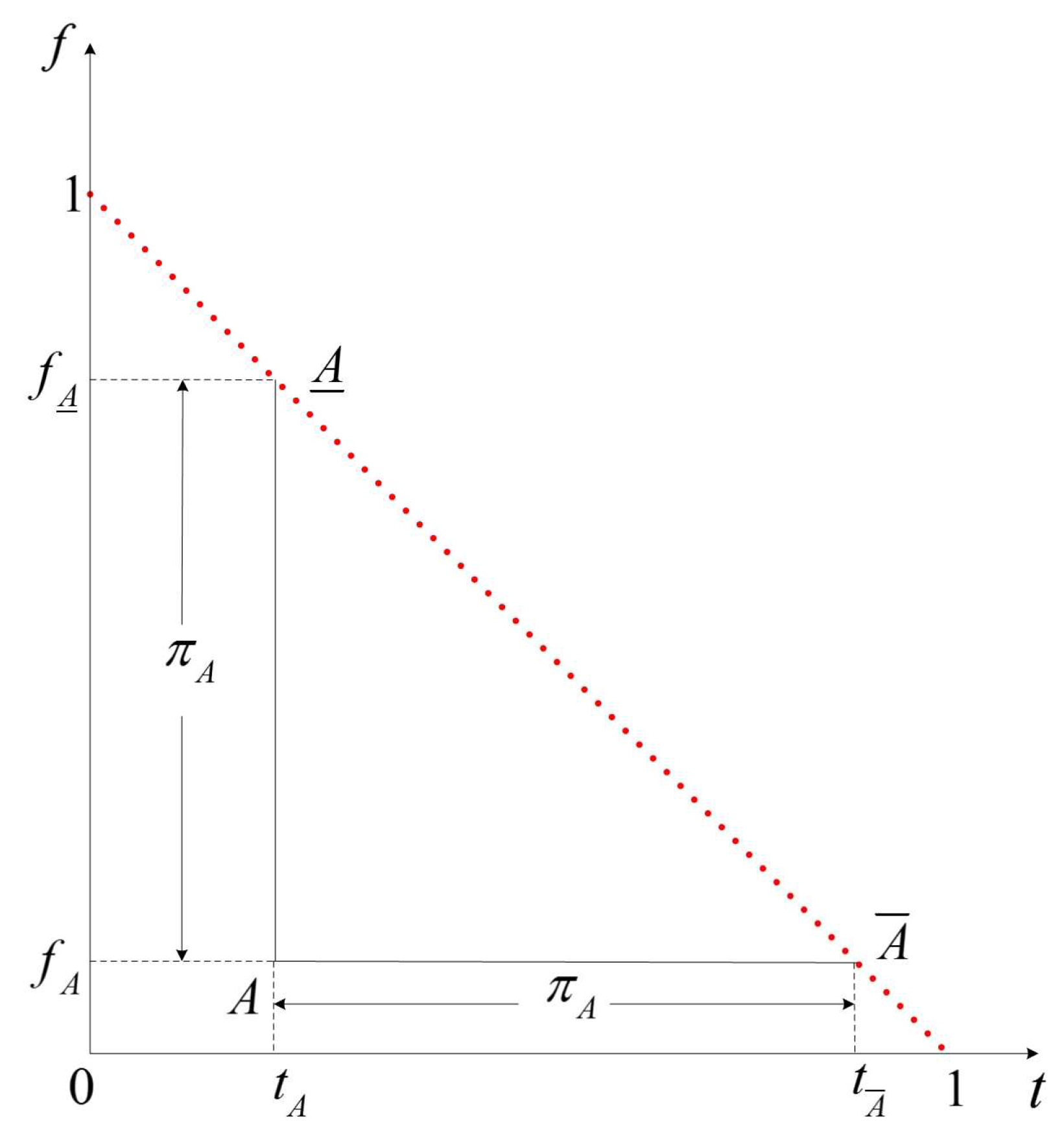
Definition 8.

Let $A=(t_A,f_A)\in L^{*}$ and ${\pi }_A=1-t_A-f_A$. Then the IFVs $\overline{A}=(t_A+{\pi }_A,f_A)$ and $\underline{A}=(t_A,f_A+{\pi }_A)$ are called the upper determination and lower determination of A, respectively.

Given an IFV $A=(t_A,f_A)\in L^{*}$ with the indeterminacy ${\pi }_A>0$. Based on the above-mentioned voting model, we consider two special cases in which the abstention can be completely eliminated. On one hand, one can assume that all the voters who previously abstained in the vote reconsider their decisions, and choose to approve the proposal. In this case, the IFV A will be increased into its upper determination $\overline{A}=(t_A+{\pi }_A,f_A)$. On the other hand, if we assume that all the voters who previously declined to vote alternatively decide to vote against the proposal. In response to this case, the IFV A will be decreased into its lower determination $\underline{A}=(t_A,f_A+{\pi }_A)$.

In addition to the above two extreme cases, there are various other ways for redistributing part or all abstention votes into either approval or rejection votes by asking the abstention voters to vote for the second time. All possible voting results obtained from such a process can be described in terms of the following notion.

Definition 9.

Let $A=(t_A,f_A)\in L^{*}$. Then

$${▵}_A=\{(t,f)\in L^{*}\mid (t_A\le t\le 1-f_A)\wedge (f_A\le f\le 1-t_A)\}$$

is called the spectrum triangle spanned by the IFV A.

It is clear that the spectrum triangle spanned by the IFV $(0,0)$ is the whole lattice $L^{*}$. Moreover, one can verify an assertion as follows.

Proposition 2.

Let $A=(t_A,f_A)\in L^{*}$. Then the following statements are equivalent:

(1)

$h_A=t_A+f_A=1$;

(2)

${\pi }_A=1-h_A=0$;

(3)

$\overline{A}=A=\underline{A}$;

(4)

${▵}_A=\left\{A\right\}$.

Proof. 

Straightforward. ☐

In various applications regarding information fusion and decision making under an intuitionistic fuzzy setting, it is an crucial issue to consider the aggregation of intuitionistic fuzzy values. By virtue of the operations given in Definition 2, Xu et al. [6] initiated the following operator which is helpful for aggregating IFVs.

Definition 10

([6]).Let ${\alpha }_i$ ($i=1,2,\cdots ,n$) be IFVs in $L^{*}$. The intuitionistic fuzzy weighted averaging (IFWA) operator of dimension n is a mapping ${\mathsf{\Xi }}_w:{\left(L^{*}\right)}^n\to L^{*}$ given by

$${\mathsf{\Xi }}_w({\alpha }_1,{\alpha }_2,\cdots ,{\alpha }_n)=w_1{\alpha }_1\oplus w_2{\alpha }_2\oplus \cdots \oplus w_n{\alpha }_n,$$

where $w={(w_1,w_2,\cdots ,w_n)}^T$ is the weight vector such that $w_i\in [0,1]$ ($i=1,2,\cdots ,n$) and ${\sum }_{i=1}^n{w}_i=1$.

Especially, if $w=\widehat{w}={(1/n,1/n,\cdots ,1/n)}^T$, then ${\mathsf{\Xi }}_{\widehat{w}}$ is simply written as $\mathsf{\Xi }$ and called the intuitionistic fuzzy averaging (IFA) operator. That is,

$$\mathsf{\Xi }({\alpha }_1,{\alpha }_2,\cdots ,{\alpha }_n)=\frac{1}{n}({\alpha }_1\oplus {\alpha }_2\oplus \cdots \oplus {\alpha }_n).$$

(4)

The following result is helpful for simplifying the calculation regarding IFWA operators.

Theorem 2.

[6] Let ${\alpha }_i=(t_{{\alpha }_i},f_{{\alpha }_i})\in L^{*}$ ($i=1,2,\cdots ,n$). Then we have

$${\mathsf{\Xi }}_w({\alpha }_1,{\alpha }_2,\cdots ,{\alpha }_n)=\left(1-\prod _{i=1}^n{(1-t_{{\alpha }_i})}^{w_i},\prod _{i=1}^n{f}_{{\alpha }_i}^{w_i}\right).$$

(5)

where $w={(w_1,w_2,\cdots ,w_n)}^T$ is the weight vector.

In order to further simplify the calculation with regard to the aggregation of IFVs, we define the following two operators.

Definition 11.

Let ${\alpha }_i=(t_{{\alpha }_i},f_{{\alpha }_i})$ ($i=1,2,\cdots ,n$) be IFVs in $L^{*}$. The simply weighted intuitionistic fuzzy averaging (SWIFA) operator of dimension n is a mapping ${\mathsf{\Xi }}_w^s:{\left(L^{*}\right)}^n\to L^{*}$ given by

$${\mathsf{\Xi }}_w^s({\alpha }_1,{\alpha }_2,\cdots ,{\alpha }_n)=\left(\sum _{i=1}^n{w}_i{t}_{{\alpha }_i},\sum _{i=1}^n{w}_i{f}_{{\alpha }_i}\right),$$

(6)

where $w={(w_1,w_2,\cdots ,w_n)}^T$ is the weight vector such that $w_i\in [0,1]$ ($i=1,2,\cdots ,n$) and ${\sum }_{i=1}^n{w}_i=1$.

In particular, ${\mathsf{\Xi }}_w^s$ with $w={(1/n,1/n,\cdots ,1/n)}^T$ is simply written as ${\mathsf{\Xi }}^s$ and called the simple intuitionistic fuzzy averaging (SIFA) operator. That is,

$${\mathsf{\Xi }}^s({\alpha }_1,{\alpha }_2,\cdots ,{\alpha }_n)=\left(\frac{1}{n}\sum _{i=1}^n{t}_{{\alpha }_i},\frac{1}{n}\sum _{i=1}^n{f}_{{\alpha }_i}\right).$$

(7)

To illustrate the distinct aggregating effects on IFVs by employing the above operators, we consider an example as follows.

Example 1.

Let ${\alpha }_1=(0.2,0.5)$, ${\alpha }_2=(0.4,0.2)$ and ${\alpha }_3=(0.3,0.3)$ be three IFVs in $L^{*}$. First, let us take $w_1={(0.3,0.5,0.2)}^T$ as the weight vector. Then according to Definition 10 and Equation (5), we have

$$\begin{array}{cc}\hfill {\mathsf{\Xi }}_{w_1}({\alpha }_1,{\alpha }_2,{\alpha }_3)& =0.3{\alpha }_1\oplus 0.5{\alpha }_2\oplus 0.3{\alpha }_3\hfill \\ \hfill & =\left(1-\prod _{i=1}^3{(1-t_{{\alpha }_i})}^{w_i},\prod _{i=1}^3{f}_{{\alpha }_i}^{w_i}\right)\hfill \\ \hfill & =\left(1-{0.8}^{0.3}\times {0.6}^{0.5}\times {0.7}^{0.2},{0.5}^{0.3}\times {0.2}^{0.5}\times {0.3}^{0.2}\right)\hfill \\ \hfill & =(0.3254,0.2855).\hfill \end{array}$$

Alternatively, according to Definition 11 and Equation (6), we have

$$\begin{array}{cc}\hfill {\mathsf{\Xi }}_{w_1}^s({\alpha }_1,{\alpha }_2,{\alpha }_3)& =\left(\sum _{i=1}^3{w}_i{t}_{{\alpha }_i},\sum _{i=1}^3{w}_i{f}_{{\alpha }_i}\right)\hfill \\ \hfill & =(0.06+0.2+0.06,0.15+0.1+0.06)\hfill \\ \hfill & =(0.3200,0.3100).\hfill \end{array}$$

Using the weight vector $w_2={(1/3,1/3,1/3)}^T$, we can get

$$\begin{array}{cc}\hfill \mathsf{\Xi }({\alpha }_1,{\alpha }_2,{\alpha }_3)& =\frac{1}{3}({\alpha }_1\oplus {\alpha }_2\oplus {\alpha }_3)\hfill \\ \hfill & =\left(1-\prod _{i=1}^3{(1-t_{{\alpha }_i})}^{1/3},\prod _{i=1}^3{f}_{{\alpha }_i}^{1/3}\right)\hfill \\ \hfill & =\left(1-{0.8}^{1/3}\times {0.6}^{1/3}\times {0.7}^{1/3},{0.5}^{1/3}\times {0.2}^{1/3}\times {0.3}^{1/3}\right)\hfill \\ \hfill & =(0.3048,0.3107)\hfill \end{array}$$

according to Equation (4). Finally, according to Equation (7), we obtain that

$$\begin{array}{cc}\hfill {\mathsf{\Xi }}^s({\alpha }_1,{\alpha }_2,{\alpha }_3)& =\left(\frac{1}{3}\sum _{i=1}^3{t}_{{\alpha }_i},\frac{1}{3}\sum _{i=1}^3{f}_{{\alpha }_i}\right)\hfill \\ \hfill & =\left(\frac{0.2+0.4+0.3}{3},\frac{0.5+0.2+0.3}{3}\right)\hfill \\ \hfill & =(0.3000,0.3333).\hfill \end{array}$$

To demonstrate the applicability of the above operators in practical cases, we consider the following example adopted from [10] with some changes.

Example 2.

Suppose that $U=\{p_1,p_2,\cdots ,p_5\}$ contains five candidates who might fit a senior faculty position at University X. In order to hire the most suitable person, a committee of experts is set up and chaired by Prof. Y as the director. This committee gives evaluation of all candidates upon the criteria in $E=\{e_1,e_2,e_3,e_4\}$. The meaning of $e_j$ ($1\le j\le 4$) is as follows:

$$\begin{array}{cc}\hfill ll{e}_1:& researchproductivity;\hfill \\ \hfill e_2:& managerialskills;\hfill \\ \hfill e_3:& impactonresearchcommunity;\hfill \\ \hfill e_4:& abilitytoworkunderpressure.\hfill \end{array}$$

The evaluation results can be described by an intuitionistic fuzzy soft set (see Definition 3.1 in [10]), as shown in

Table 1. Intuitionistic fuzzy soft set $\mathfrak{I}=(\tilde{F},E)$.

U	${\mathit{e}}_1$	${\mathit{e}}_2$	${\mathit{e}}_3$	${\mathit{e}}_4$
$p_1$	$(0.8,0.1)$	$(0.6,0.2)$	$(0.4,0.4)$	$(0.7,0.2)$
$p_2$	$(0.6,0.2)$	$(0.7,0.2)$	$(0.4,0.5)$	$(0.5,0.1)$
$p_3$	$(0.7,0.3)$	$(0.8,0.1)$	$(0.6,0.3)$	$(0.7,0.1)$
$p_4$	$(0.8,0.1)$	$(0.9,0.1)$	$(0.6,0.2)$	$(0.5,0.3)$
$p_5$	$(0.5,0.4)$	$(0.6,0.3)$	$(0.7,0.2)$	$(0.2,0.6)$

. Assume that the weight vector

$$w={(0.2,0.35,0.2,0.25)}^T$$

(8)

is provided by Prof. Y, the director of the evaluation committee. Then we can use the proposed operators to determine the aggregated IFVs of all candidates. If we use the SWIFA operator, the aggregated IFVs $Z_i$ can be calculated by

$$Z_i={\mathsf{\Xi }}_w^s({\alpha }_{i1},{\alpha }_{i2},{\alpha }_{i3},{\alpha }_{i4})=\left(\sum _{j=1}^4{w}_j{t}_{{\alpha }_{ij}},\sum _{j=1}^4{w}_j{f}_{{\alpha }_{ij}}\right),$$

(9)

where ${\alpha }_{ij}=\tilde{F}\left(e_j\right)\left(p_i\right)=(t_{{\alpha }_{ij}},f_{{\alpha }_{ij}})$, $1\le i\le 5$ and $1\le j\le 4$.

By calculation, we can obtain the following aggregated IFVs:

$$\begin{array}{cc}\hfill Z_1& =(0.6250,0.2200),\hfill \\ \hfill Z_2& =(0.5700,0.2350),\hfill \\ \hfill Z_3& =(0.7150,0.1800),\hfill \\ \hfill Z_4& =(0.7200,0.1700),\hfill \\ \hfill Z_5& =(0.5000,0.3750).\hfill \end{array}$$

According to Definition 3, we have $s_{Z_1}=0.4050$, $s_{Z_2}=0.3350$, $s_{Z_3}=0.5350$, $s_{Z_4}=0.5500$ and $s_{Z_5}=0.1250$. Using Definition 4, we get $h_{Z_1}=0.8450$, $h_{Z_2}=0.8050$, $h_{Z_3}=0.8950$, $h_{Z_4}=0.8900$ and $h_{Z_5}=0.8750$.

Based on Xu and Yager’s admissible order ${\le }_{(s,h)}$, we have

$$Z_5{\le }_{(s,h)}{Z}_2{\le }_{(s,h)}{Z}_1{\le }_{(s,h)}{Z}_3{\le }_{(s,h)}{Z}_4.$$

The five candidates are finally ranked as follows:

$$p_4\succ p_3\succ p_1\succ p_2\succ p_5.$$

Therefore, $p_4$ is the most suitable candidate for the senior faculty position.

It is worth noting that other operators can be used to replace the SWIFA operator in Equation (9) for determining the aggregated IFVs. In addition, we can also rank the aggregated IFVs by means of other admissible orders.

Definition 12.

Let ${\mathsf{\Xi }}_w:{\left(L^{*}\right)}^3\to L^{*}$ be an IFWA operator with the weight vector $w=(w_1,w_2,w_3)$. The weighted centroid transformation (WCT) of IFVs is a mapping ${\mathsf{\Gamma }}_w:L^{*}\to L^{*}$ given by

$${\mathsf{\Gamma }}_w\left(A\right)={\mathsf{\Xi }}_w(\underline{A},A,\overline{A}),$$

where $A=(t_A,f_A)\in L^{*}$.

In particular, if ${\mathsf{\Xi }}_w$ is replaced by the IFA operator $\mathsf{\Xi }$ with the weight vector $\widehat{w}={(1/3,1/3,1/3)}^T$, then ${\mathsf{\Gamma }}_{\widehat{w}}\left(A\right)$ is denoted by $\mathsf{\Gamma }\left(A\right)$ and called the centroid transformation of IFVs. That is,

$$\mathsf{\Gamma }\left(A\right)=\frac{1}{3}(\underline{A}\oplus A\oplus \overline{A}).$$

(10)

By Definition 8 and the Equation (5) in Theorem 2, we can deduce the following formula for calculation of the weighted centroid transformation.

Proposition 3.

Let $A=(t_A,f_A)\in L^{*}$ and $w=(w_1,w_2,w_3)$ be the weight vector. Then we have

$${\mathsf{\Gamma }}_w\left(A\right)=\left(1-{(1-t_A)}^{w_1+w_2}·{f_A}^{w_3},{(1-t_A)}^{w_1}·{f_A}^{w_2+w_3}\right).$$

(11)

Proof. 

Let $A=(t_A,f_A)\in L^{*}$. According to Definition 8, we get the upper determination

$$\overline{A}=(t_{\overline{A}},f_{\overline{A}})=(t_A+{\pi }_A,f_A)=(1-f_A,f_A)$$

and the lower determination

$$\underline{A}=(t_{\underline{A}},f_{\underline{A}})=(t_A,f_A+{\pi }_A)=(t_A,1-t_A).$$

From Definition 12 and Equation (5), it follows that

$$\begin{array}{c}\hfill \begin{array}{cc}\hfill {\mathsf{\Gamma }}_w\left(A\right)& ={\mathsf{\Xi }}_w(\underline{A},A,\overline{A})\hfill \\ & =\left(1-{(1-t_{\underline{A}})}^{w_1}·{(1-t_A)}^{w_2}·{(1-t_{\overline{A}})}^{w_3},f_{\underline{A}}^{w_1}·f_A^{w_2}·f_{\overline{A}}^{w_3}\right)\hfill \\ & =\left(1-{(1-t_A)}^{w_1+w_2}·{f_A}^{w_3},{(1-t_A)}^{w_1}·{f_A}^{w_2+w_3}\right),\hfill \end{array}\end{array}$$

where $w=(w_1,w_2,w_3)$ is the weight vector. ☐

As an immediate consequence of Proposition 3, we can obtain the following formula regarding the centroid transformation.

Proposition 4.

Let $A=(t_A,f_A)\in L^{*}$. Then we have

$$\mathsf{\Gamma }\left(A\right)=\left(1-{(1-t_A)}^{2/3}·{f_A}^{1/3},{(1-t_A)}^{1/3}·{f_A}^{2/3}\right).$$

(12)

Definition 13.

Let ${\mathsf{\Xi }}_w^s:{\left(L^{*}\right)}^3\to L^{*}$ be an SWIFA operator with the weight vector $w=(w_1,w_2,w_3)$. The simply weighted centroid transformation (SWCT) of IFVs is a mapping ${\mathsf{\Gamma }}_w^s:L^{*}\to L^{*}$ given by

$${\mathsf{\Gamma }}_w^s\left(A\right)={\mathsf{\Xi }}_w^s(\underline{A},A,\overline{A}),$$

where $A=(t_A,f_A)\in L^{*}$.

Proposition 5.

Let $A=(t_A,f_A)\in L^{*}$ and ${\pi }_A=1-h_A$. Then

$$\begin{array}{cc}\hfill {\mathsf{\Gamma }}_w^s\left(A\right)& =\left(t_A+w_3{\pi }_A,f_A+w_1{\pi }_A\right)\hfill \\ \hfill & =\left((1-w_3)t_A+w_3(1-f_A),w_1(1-t_A)+(1-w_1)f_A\right),\hfill \end{array}$$

where $w=(w_1,w_2,w_3)$ is the weight vector.

Proof. 

Let $A=(t_A,f_A)\in L^{*}$. Note first that

$$\overline{A}=(t_{\overline{A}},f_{\overline{A}})=(t_A+{\pi }_A,f_A)=(1-f_A,f_A)$$

and

$$\underline{A}=(t_{\underline{A}},f_{\underline{A}})=(t_A,f_A+{\pi }_A)=(t_A,1-t_A),$$

according to Definition 8.

Using Definition 13 and Equation (6), we deduce that

$$\begin{array}{ccc}\hfill {\mathsf{\Gamma }}_w^s\left(A\right)& =& {\mathsf{\Xi }}_w^s(\underline{A},A,\overline{A})=\left(w_1{t}_{\underline{A}}+w_2{t}_A+w_3{t}_{\overline{A}},w_1{f}_{\underline{A}}+w_2{f}_A+w_3{f}_{\overline{A}}\right)\hfill \\ & =& \left((w_1+w_2+w_3)t_A+w_3{\pi }_A,(w_1+w_2+w_3)f_A+w_1{\pi }_A\right)\hfill \\ & =& \left(t_A+w_3{\pi }_A,f_A+w_1{\pi }_A\right).\hfill \end{array}$$

Note also that ${\pi }_A=1-h_A=1-t_A-f_A$. Thus we have

$$\begin{array}{ccc}\hfill {\mathsf{\Gamma }}^s\left(A\right)& =& {\mathsf{\Xi }}^s(\underline{A},A,\overline{A})=\left(t_A+w_3{\pi }_A,f_A+w_1{\pi }_A\right)\hfill \\ & =& \left(t_A+w_3(1-t_A-f_A),f_A+w_1(1-t_A-f_A)\right)\hfill \\ & =& \left(t_A-w_3{t}_A+w_3(1-f_A),f_A-w_1{f}_A+w_1(1-t_A)\right)\hfill \\ & =& \left((1-w_3)t_A+w_3(1-f_A),w_1(1-t_A)+(1-w_1)f_A\right),\hfill \end{array}$$

which completes the proof. ☐

5. Limits of Simple Centroid Transformations Sequences

Chen et al. [14] proposed a novel similarity measure between intuitionistic fuzzy sets for coping with pattern recognition problems. In fact, their similarity measure is based on a transformation as follows.

Definition 14.

The simple centroid transformation (SCT) of IFVs is a mapping ${\mathsf{\Gamma }}^s:L^{*}\to L^{*}$ given by

$${\mathsf{\Gamma }}^s\left(A\right)={\mathsf{\Xi }}^s(\underline{A},A,\overline{A}),$$

where $A=(t_A,f_A)\in L^{*}$.

By Definition 14 and Proposition 5, we can get the following formula for convenient calculation of the simple centroid transformation.

Proposition 6.

Let $A=(t_A,f_A)\in L^{*}$ and ${\pi }_A=1-h_A$. Then

$${\mathsf{\Gamma }}^s\left(A\right)=\left(t_A+\frac{{\pi }_A}{3},f_A+\frac{{\pi }_A}{3}\right)=\left(\frac{1+2t_A-f_A}{3},\frac{1+2f_A-t_A}{3}\right).$$

(13)

Proof. 

This follows directly from Proposition 5. ☐

Let $A=(t_A,f_A)\in L^{*}$ with ${\pi }_A>0$. It is interesting to see that the image ${\mathsf{\Gamma }}^s\left(A\right)$ of the IFV A under SCT is exactly the geometric centroid of the spectrum triangle ${▵}_A$ spanned by A. This gives a geometric interpretation of SCT as illustrated by Figure 2.

Example 3.

Let $A=(0.2,0.6)$ be an IFV in $L^{*}$ and $w_1={(0.3,0.5,0.2)}^T$ be the weight vector. According to Definition 12 and Equation (11), we have

$$\begin{array}{cc}\hfill {\mathsf{\Gamma }}_w\left(A\right)& ={\mathsf{\Xi }}_w(\underline{A},A,\overline{A})\hfill \\ & =\left(1-{(1-t_A)}^{0.8}·{f_A}^{0.2},{(1-t_A)}^{0.3}·{f_A}^{0.7}\right)\hfill \\ & =\left(1-{0.8}^{0.8}\times {0.6}^{0.2},{0.8}^{0.3}\times {0.6}^{0.7}\right)\hfill \\ & =(0.2447,0.6541).\hfill \end{array}$$

By Equation (12) and the definition of centroid transformations, we obtain that

$$\begin{array}{cc}\hfill \mathsf{\Gamma }\left(A\right)& =\frac{1}{3}(\underline{A}\oplus A\oplus \overline{A})\hfill \\ & =\left(1-{(1-t_A)}^{2/3}·{f_A}^{1/3},{(1-t_A)}^{1/3}·{f_A}^{2/3}\right)\hfill \\ & =\left(1-{0.8}^{2/3}\times {0.6}^{1/3},{0.8}^{1/3}\times {0.6}^{2/3}\right)\hfill \\ & =(0.2732,0.6604).\hfill \end{array}$$

Next, according to Definition 13 and Proposition 5, we have

$$\begin{array}{cc}\hfill {\mathsf{\Gamma }}_w^s\left(A\right)& ={\mathsf{\Xi }}_w^s(\underline{A},A,\overline{A})=\left(0.8t_A+0.2(1-f_A),0.3(1-t_A)+0.7f_A\right)\hfill \\ & =\left(0.8\times 0.2+0.2\times 0.4,0.3\times 0.8+0.7\times 0.6\right)\hfill \\ & =(0.2400,0.6600).\hfill \end{array}$$

Finally, Definition 14 and Equation (13), we obtain that

$$\begin{array}{cc}\hfill {\mathsf{\Gamma }}^s\left(A\right)& ={\mathsf{\Xi }}^s(\underline{A},A,\overline{A})=\left(\frac{1+2t_A-f_A}{3},\frac{1+2f_A-t_A}{3}\right)\hfill \\ & =\left(\frac{1+2\times 0.2-0.6}{3},\frac{1+2\times 0.6-0.2}{3}\right)\hfill \\ & =(0.2667,0.6667).\hfill \end{array}$$

The above illustrating example reveals the distinct results obtained by employing diverse kinds of centroid transformations presented in the foregoing.

Proposition 7.

Let $A=(t_A,f_A)\in L^{*}$ and $B={\mathsf{\Gamma }}^s\left(A\right)=(t_B,f_B)$. Then

(1)

$s_A=t_A-f_A=t_B-f_B=s_B$;

(2)

${\delta }_A=(s_A+1)/2=(s_B+1)/2={\delta }_B$;

(3)

$h_B=h_A+2{\pi }_A/3=(2+h_A)/3$;

(4)

${\pi }_B=(1-h_A)/3={\pi }_A/3$.

Proof. 

Let $A=(t_A,f_A)\in L^{*}$. By Proposition 6, we have

$$B={\mathsf{\Gamma }}^s\left(A\right)=(t_B,f_B)=\left(t_A+\frac{{\pi }_A}{3},f_A+\frac{{\pi }_A}{3}\right).$$

From Definition 3, it follows that

$$s_B=t_B-f_B=(t_A+\frac{{\pi }_A}{3})-(f_A+\frac{{\pi }_A}{3})=t_A-f_A=s_A,$$

which shows that the first assertion is true.

Then the second assertion follows directly from the first statement.

Next, by Definition 4 we have

$$h_B=t_B+f_B=(t_A+\frac{{\pi }_A}{3})+(f_A+\frac{{\pi }_A}{3})=h_A+\frac{2{\pi }_A}{3}.$$

Note also that ${\pi }_A=1-h_A$. Thus we deduce that

$$h_B=h_A+\frac{2{\pi }_A}{3}=\frac{3h_A+2(1-h_A)}{3}=\frac{2+h_A}{3},$$

which shows that the third assertion holds.

Finally, using the above result it follows that

$${\pi }_B=1-h_B=1-\frac{2+h_A}{3}=\frac{1-h_A}{3}=\frac{{\pi }_A}{3},$$

which completes the proof. ☐

The above results reveal that the score will not be changed, while the accuracy does not decrease after performing the SCT on a given IFV. As an immediate consequence, we have the following assertion.

Proposition 8.

Let $A\in L^{*}$ and $B={\mathsf{\Gamma }}^s\left(A\right)$. Then we have $A{\le }_{(s,h)}B$.

Proof. 

This follows directly from Proposition 7. ☐

This means that an IFV will become greater in the sense of Xu’s partial order after performing the simple centroid transformation.

Definition 15.

Let $A_1\in L^{*}$ and $A_{n+1}={\mathsf{\Gamma }}^s\left(A_n\right)$ ($n=1,2,\cdots$). The IFV sequence ${\left\{A_n\right\}}_{n=1}^{\infty }$ is called the simple centroid transformation sequence (SCTS) derived from the IFV $A_1$.

Proposition 9.

Let $A_1\in L^{*}$ and ${\left\{A_n\right\}}_{n=1}^{\infty }$ be the SCTS derived from $A_1$. Then we have

(1)

$(0,1){\le }_{(s,h)}{A}_n{\le }_{(s,h)}(1,0)$;

(2)

$A_n{\le }_{(s,h)}{A}_{n+1}$,

where n is any positive integer.

Proof. 

This follows directly from Definition 7 and Proposition 8. ☐

Let $A_1=(t_{A_1},f_{A_1})$ be any chosen but fixed IFV in $L^{*}$. After performing the SCT, we obtain another IFV $A_2=(t_{A_2},f_{A_2})\in L^{*}$ with

$$t_{A_2}=t_{A_1}+\frac{{\pi }_{A_1}}{3}=\frac{1+2t_{A_1}-f_{A_1}}{3}$$

and

$$f_{A_2}=f_{A_1}+\frac{{\pi }_{A_1}}{3}=\frac{1+2f_{A_1}-t_{A_1}}{3}.$$

Using the IFV $A_2$ as the new input and perform the SCT once again, we get the IFV $A_3=(t_{A_3},f_{A_3})\in L^{*}$ with

$$t_{A_3}=t_{A_2}+\frac{{\pi }_{A_2}}{3}=\frac{1+2t_{A_2}-f_{A_2}}{3}=t_{A_1}+\frac{{\pi }_{A_1}}{3}+\frac{{\pi }_{A_2}}{3}$$

and

$$f_{A_3}=f_{A_2}+\frac{{\pi }_{A_2}}{3}=\frac{1+2f_{A_2}-t_{A_2}}{3}=f_{A_1}+\frac{{\pi }_{A_1}}{3}+\frac{{\pi }_{A_2}}{3}.$$

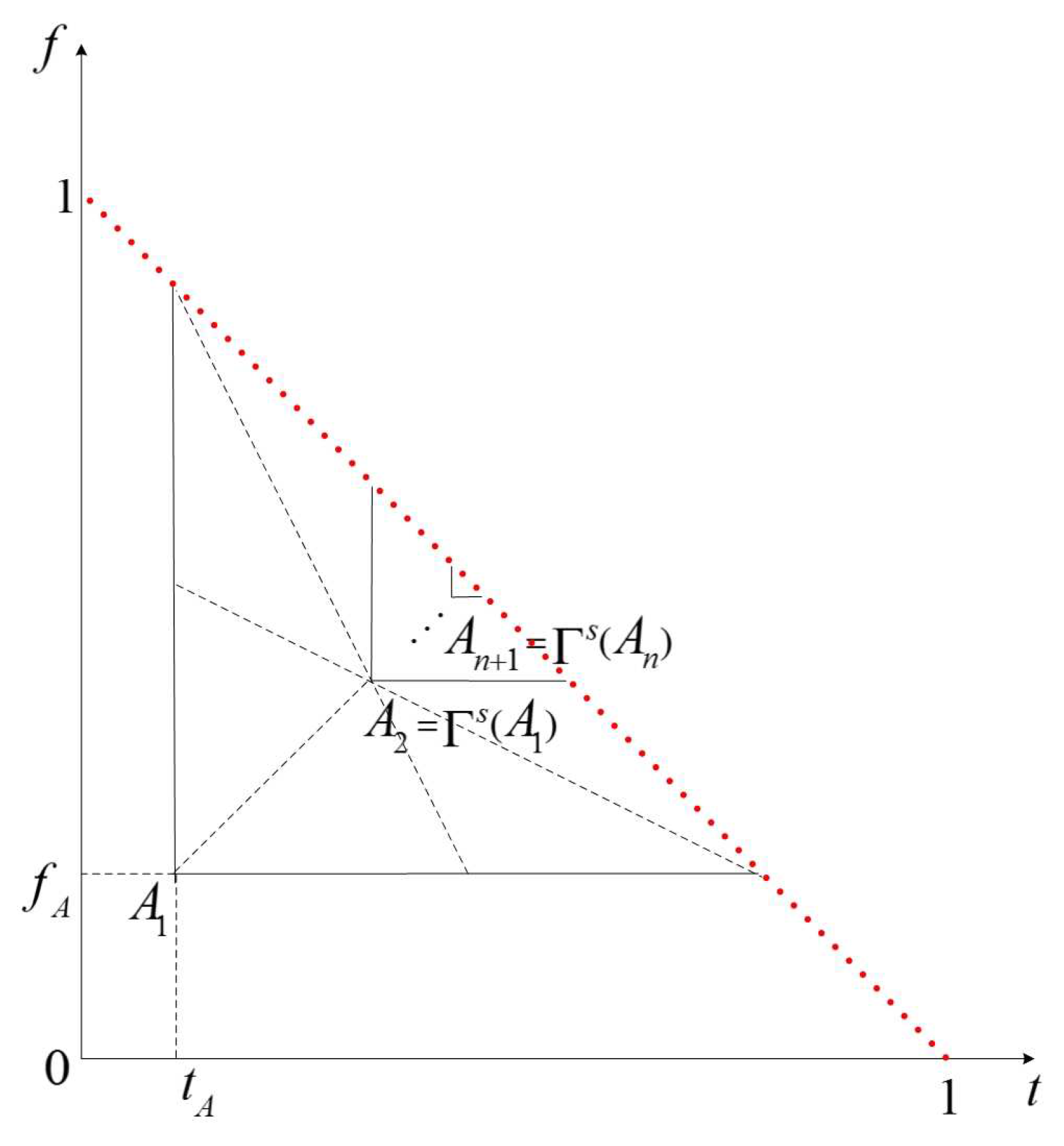
By applying the SCT repeatedly, we can get a sequence of IFVs:

$$A_1,A_2,\cdots ,A_n,A_{n+1}={\mathsf{\Gamma }}^s\left(A_n\right),\cdots .$$

That is, the SCTS ${\left\{A_n\right\}}_{n=1}^{\infty }$ derived from the IFV $A_1$. The geometric illustration of this process is shown in Figure 3.

Considering the spectrum triangles spanned by the IFVs $A_n$ in the simple centroid transformation sequence, we introduce a notion as follows.

Definition 16.

Let $A_1\in L^{*}$ and ${\left\{A_n\right\}}_{n=1}^{\infty }$ be the SCTS derived from $A_1$. The sequence ${\left\{{▵}_{A_n}\right\}}_{n=1}^{\infty }$ is called the spectrum triangle sequence (STS) derived from the IFV $A_1$.

Proposition 10.

Let $A_1\in L^{*}$ and ${\left\{{▵}_{A_n}\right\}}_{n=1}^{\infty }$ be the STS derived from $A_1$. If we denote by $a_n$ the area of the triangle ${▵}_{A_n}$, then ${\left\{a_n\right\}}_{n=1}^{\infty }$ is a non-increasing sequence with $\underset{n\to \infty }{lim}{a}_n=0$.

Proof. 

Note first that $a_n={\pi }_{A_n}^2/2$ for all positive integer n. By Proposition 7, we can deduce that

$$a_{n+1}=\frac{{\pi }_{A_{n+1}}^2}{2}=\frac{1}{2}{\left(\frac{{\pi }_{A_n}}{3}\right)}^2=\frac{a_n}{9}.$$

Thus ${\left\{a_n\right\}}_{n=1}^{\infty }$ is a non-increasing sequence with lower bound 0. Hence the sequence ${\left\{a_n\right\}}_{n=1}^{\infty }$ must converge to its limit $\underset{n\to \infty }{lim}{a}_n=a$. It follows that $a=a/9$ and so $a=\underset{n\to \infty }{lim}{a}_n=0$. ☐

Proposition 11.

Let $A_1=(t_{A_1},f_{A_1})\in L^{*}$ and ${\{A_n=(t_{A_n},f_{A_n})\}}_{n=1}^{\infty }$ be the SCTS derived from $A_1$. Then ${\left\{s_{A_n}\right\}}_{n=1}^{\infty }$ is a constant sequence and

$$\underset{n\to \infty }{lim}{s}_{A_n}=\underset{n\to \infty }{lim}(t_{A_n}-f_{A_n})=t_{A_1}-f_{A_1}.$$

Proof. 

This follows directly from Proposition 7. ☐

Proposition 12.

Let $A_1=(t_{A_1},f_{A_1})\in L^{*}$ and ${\{A_n=(t_{A_n},f_{A_n})\}}_{n=1}^{\infty }$ be the SCTS derived from $A_1$. Then ${\left\{h_{A_n}\right\}}_{n=1}^{\infty }$ is a non-decreasing sequence and

$$\underset{n\to \infty }{lim}{h}_{A_n}=\underset{n\to \infty }{lim}(t_{A_n}+f_{A_n})=1.$$

Proof. 

It is easy to see that $0\le h_{A_n}\le 1$ ($n=1,2,\cdots$) by the definition of accuracy function. This shows that ${\left\{h_{A_n}\right\}}_{n=1}^{\infty }$ is a bounded sequence with upper bound 1. By Proposition 7, we have

$$h_{A_{n+1}}=h_{A_n}+\frac{2{\pi }_{A_n}}{3}$$

for any positive integer n. Thus

$$h_{A_{n+1}}-h_{A_n}=\frac{2{\pi }_{A_n}}{3}\ge 0,$$

and so ${\left\{h_{A_n}\right\}}_{n=1}^{\infty }$ is a non-decreasing sequence. Now we assume that $\underset{n\to \infty }{lim}{h}_{A_n}=a$. By Proposition 7, we also have

$$h_{A_{n+1}}=\frac{2+h_{A_n}}{3}.$$

It follows that $a=(2+a)/3$ and so $a=\underset{n\to \infty }{lim}{h}_{A_n}=1$. ☐

The above statement indicates that the indeterminacies of the IFVs successively obtained by the sequential application of simple centroid transformations converge to zero. In addition, the following result shows that the membership grades $t_{A_n}$ of the IFVs in this sequence converge to the number ${\delta }_{A_1}$, namely the image of the initial IFV $A_1$ under the expectation score function.

Theorem 3.

Let $A_1=(t_{A_1},f_{A_1})\in L^{*}$ and ${\{A_n=(t_{A_n},f_{A_n})\}}_{n=1}^{\infty }$ be the SCTS derived from $A_1$. Then

$$\underset{n\to \infty }{lim}{t}_{A_n}=t_{A_1}+\frac{{\pi }_{A_1}}{2}=\frac{t_{A_1}-f_{A_1}+1}{2}={\delta }_{A_1}$$

and

$$\underset{n\to \infty }{lim}{f}_{A_n}=f_{A_1}+\frac{{\pi }_{A_1}}{2}=\frac{f_{A_1}-t_{A_1}+1}{2}=1-{\delta }_{A_1}.$$

Proof. 

By induction on the positive integer n, it is easy to verify that

$$t_{A_n}=t_{A_1}+\frac{1}{3}\sum _{i=1}^{n-1}{\pi }_{A_i}$$

and

$$f_{A_n}=f_{A_1}+\frac{1}{3}\sum _{i=1}^{n-1}{\pi }_{A_i}.$$

By Proposition 7, we also have ${\pi }_{A_{n+1}}={\pi }_{A_n}/3$, which indicates that ${\left\{{\pi }_{A_n}\right\}}_{n=1}^{\infty }$ is a geometric sequence. Hence we further deduce that

$$\underset{n\to \infty }{lim}\sum _{i=1}^{n-1}{\pi }_{A_i}=\sum _{i=1}^{\infty }{\pi }_{A_i}=\frac{{\pi }_{A_1}}{1-1/3}=\frac{3{\pi }_{A_1}}{2}.$$

Using basic properties of the limit of sequences, it follows that

$$\begin{array}{cc}\hfill \underset{n\to \infty }{lim}{t}_{A_n}& =\underset{n\to \infty }{lim}\left(t_{A_1}+\frac{1}{3}\sum _{i=1}^{n-1}{\pi }_{A_i}\right)\hfill \\ \hfill & =t_{A_1}+\frac{1}{3}\underset{n\to \infty }{lim}\sum _{i=1}^{n-1}{\pi }_{A_i}\hfill \\ \hfill & =t_{A_1}+\frac{{\pi }_{A_1}}{2}\hfill \\ \hfill & =\frac{2t_{A_1}+(1-t_{A_1}-f_{A_1})}{2}\hfill \\ \hfill & =\frac{t_{A_1}-f_{A_1}+1}{2}={\delta }_{A_1}.\hfill \end{array}$$

In a similar fashion, it can be shown that

$$\underset{n\to \infty }{lim}{f}_{A_n}=f_{A_1}+\frac{{\pi }_{A_1}}{2}=\frac{f_{A_1}-t_{A_1}+1}{2}=1-{\delta }_{A_1},$$

which completes the proof. ☐

In the end, we can deduce the following fact which says that the IFVs in a simple centroid transformation sequence ${\left\{A_n\right\}}_{n=1}^{\infty }$ converge to the simple intuitionistic fuzzy average of the lower and upper determinations of the first IFV $A_1$ in the sequence.

Theorem 4.

Let ${\left\{A_n\right\}}_{n=1}^{\infty }$ be the SCTS derived from an IFV $A_1\in L^{*}$. Then we have

$$\underset{n\to \infty }{lim}{A}_n={\mathsf{\Xi }}^s(\underline{A_1},\overline{A_1}).$$

Proof. 

Let $A_1=(t_{A_1},f_{A_1})$. Then we have

$$\overline{A_1}=(t_{\overline{A_1}},f_{\overline{A_1}})=(t_{A_1}+{\pi }_{A_1},f_{A_1})=(1-f_{A_1},f_{A_1})$$

and

$$\underline{A_1}=(t_{\underline{A_1}},f_{\underline{A_1}})=(t_{A_1},f_{A_1}+{\pi }_{A_1})=(t_{A_1},1-t_{A_1}),$$

according to Definition 8. By Definition 8 and Equation (7), we can get

$$\begin{array}{cc}\hfill {\mathsf{\Xi }}^s(\underline{A_1},\overline{A_1})& =\left(\frac{t_{\overline{A_1}}+t_{\underline{A_1}}}{2},\frac{f_{\underline{A_1}}+f_{\overline{A_1}}}{2}\right)\hfill \\ & =\left(t_{A_1}+\frac{{\pi }_{A_1}}{2},f_{A_1}+\frac{{\pi }_{A_1}}{2}\right)\hfill \\ & =\left(\frac{t_{A_1}-f_{A_1}+1}{2},\frac{f_{A_1}-t_{A_1}+1}{2}\right)\hfill \\ & =\left({\delta }_{A_1},1-{\delta }_{A_1}\right).\hfill \end{array}$$

Note also that

$$\underset{n\to \infty }{lim}{A}_n=({\delta }_{A_1},1-{\delta }_{A_1}),$$

by Theorem 3. Thus it follows that

$$\underset{n\to \infty }{lim}{A}_n=({\delta }_{A_1},1-{\delta }_{A_1})={\mathsf{\Xi }}^s(\underline{A_1},\overline{A_1}),$$

completing the proof. ☐

6. Conclusions

Intuitionistic fuzzy sets can capture bipolar information in terms of the membership and non-membership functions. IFVs which combine membership grades with non-membership grades, could be extremely useful for developing the intuitionistic fuzzy set theory and related practice. In this study, we have defined and examined a variety of centroid transformations of IFVs. Some fundamental characterizations concerning various types of centroid transformations were presented. We also introduced the concept of simple centroid transformation sequences and investigated some properties regarding its convergence. In particular, it has been shown that the IFVs in a SCTS converge to the simple intuitionistic fuzzy average of the lower and upper determinations of the first IFV in the sequence. As future work, it would be interesting to consider how to use centroid transformations and related notions to solve multiple attribute decision making problems in an intuitionistic fuzzy setting.