Application of Tempered-Stable Time Fractional-Derivative Model to Upscale Subdiffusion for Pollutant Transport in Field-Scale Discrete Fracture Networks

Abstract

Fractional calculus provides efficient physical models to quantify non-Fickian dynamics broadly observed within the Earth system. The potential advantages of using fractional partial differential equations (fPDEs) for real-world problems are often limited by the current lack of understanding of how earth system properties influence observed non-Fickian dynamics. This study explores non-Fickian dynamics for pollutant transport in field-scale discrete fracture networks (DFNs), by investigating how fracture and rock matrix properties influence the leading and tailing edges of pollutant breakthrough curves (BTCs). Fractured reservoirs exhibit erratic internal structures and multi-scale heterogeneity, resulting in complex non-Fickian dynamics. A Monte Carlo approach is used to simulate pollutant transport through DFNs with a systematic variation of system properties, and the resultant non-Fickian transport is upscaled using a tempered-stable fractional in time advection–dispersion equation. Numerical results serve as a basis for determining both qualitative and quantitative relationships between BTC characteristics and model parameters, in addition to the impacts of fracture density, orientation, and rock matrix permeability on non-Fickian dynamics. The observed impacts of medium heterogeneity on tracer transport at late times tend to enhance the applicability of fPDEs that may be parameterized using measurable fracture–matrix characteristics.

1. Introduction

Fractional calculus, defined by non-integer order derivatives and integrals, has been applied to problems involving non-Fickian or anomalous dynamics for almost three decades [1,2]. Despite their vast potential, both theoretical development and real-world applications of fractional partial differential equations (fPDEs) have been commonly constrained by the lack of understanding of how earth system properties influence non-Fickian transport dynamics, especially for the hydrologic sciences [3]. This major challenge has historically reduced fPDEs to curve-fitting mathematical exercises, instead of routine hydrological modeling tools [4]. Intensive efforts are needed to link medium properties and the fPDE model parameters, and the commonly used Monte Carlo approach is particularly suitable for providing target dynamics for heterogeneous systems with well-controlled and definable properties.

Applications of fPDEs in the hydrologic sciences have a relatively shorter history, compared to the other stochastic hydrologic approaches, such as the single or multiple rate mobile–immobile models used extensively in chemical engineering and hydrogeology [5,6]. Anomalous transport has been observed in a variety of disordered systems in natural geological media, especially in heterogeneous porous media and fractured formations [6,7,8,9,10]. After Benson et al. [11] first introduced the spatial fractional advection–dispersion equation (fADE) to capture super-diffusive transport in sand tanks and a relatively homogenous aquifer, the fADEs had been applied to model anomalous transport in saturated, heterogeneous porous media [12,13,14,15] and Earth surfaces, such as natural rivers [16,17,18]. Applications of fADEs for flow and transport in fractured media are rather rare [19,20], although fractures are ubiquitous in geologic systems. More than 90% of natural aquifers are fractured.

Fractured media exhibit erratic heterogeneity and scale-dependent dynamics for flow and transport [21,22], challenging standard modeling tools and providing an ideal test case for fPDEs. Accurate and efficient simulation of contaminant transport within a fractured rock mass is practically important, since fractures play a large role in many natural and engineered processes, such as long-term disposal of high-level radioactive wastes in a geologic repository [21,23,24,25]. Fracture properties of natural rocks, such as fracture density, spatial location, length, aperture and orientation distributions, account for medium heterogeneity and result in non-Fickian contaminant transport [26,27,28,29], where the feasibility of fADEs and the potential correlation between fracture properties and fADE parameters have not been fully understood (see pioneer work in [19,20]).

This study selected the fPDE to quantify pollutant transport through field-scale fractured rock. Due to the prohibitive computational burden in mapping each individual fracture in standard grid-based models [20], different transport models have been developed to describe and predict complex transport behavior in fractured media at different scales [30,31,32,33]. For example, the fractured medium was treated as an equivalent continuum and the advection-dispersion equation (ADE) with ensemble averaged parameters was used to model contaminant transport [22,34]. However, the equivalent continuum assumption may only be valid for rocks with sufficiently high fracture densities that approximate an equivalent porous medium [35]. This condition is rare in natural fractured rock, while sparsely-fractured rock is more common, and favored for geological disposal [35,36]. Unlike the advection–dispersion equation (ADE), which characterizes Fickian diffusion at local scales, non-Fickian transport behaviors and asymmetric plumes, due to heterogeneity in fractures, have been observed in both the laboratory experiments and field tests [7,31,37]. This provides our motivation to select a non-local fADE in this study, which can account for both spatial and temporal nonlocal processes [38,39,40,41] in describing non-Fickian transport in fractured media.

The rest of the paper is organized as follows. In Section 2, we present the Monte Carlo approach used to simulate multiple discrete fracture network (DFN) flow and transport scenarios. The DFN is an efficient and conceptually robust numerical approach to simulate the dynamics of flow and transport in fractured media with definable fracture properties. It assumes that the rock mass is dissected by a network of discrete fractures, and that fluid flow and contaminant transport in a low-permeability rock mass are controlled by geometric and hydraulic properties of interconnected fractures of a network [42,43]. Results of the Monte Carlo simulations and applications of the fADE are then shown in Section 3. In Section 4, we explore the emergence of anomalous transport and its characterization, to gain insight into the effective solute dynamics and major mechanisms behind the observed anomalous behavior. We focus on the impact of fracture density and orientation and rock matrix permeability on non-Fickian dynamics and the fADE parameters. Section 5 draws the main conclusions.

2. Monte Carlo Simulations and the Fractional Advection–Dispersion Equation

The Monte Carlo approach utilized in this study contains three major steps. First, we generated multiple scenarios of stochastic fracture networks, with varying properties, using HydroGeoSphere (HGS) software (v.111, Aquanty Inc., Waterloo, ON, Canada) [44], which is a multi-dimensional, control–volume, finite element simulator designed to quantify the hydrologic cycle, including simulating flow and transport in fracture networks embedded in a porous medium with the discrete facture (DF) approach. Second, groundwater flow through the generated DFNs was modeled, which was expected to lead to strongly non-Fickian dynamics for conservative tracer transport (see further discussion below), providing the synthetic data to evaluate the influence of the fractured media properties on non-Fickian dynamics. Third, pollutant transport, characterized by breakthrough curves (BTCs), was then accounted for by a truncated power–law distribution memory function embodied in the fADE model. FracFit [41], a robust parameter estimation tool using a weighted nonlinear least squares (WNLS) algorithm, was used to parameterize our fractional calculus model, which could capture salient features of anomalous transport, such as skewness and power-law tails. Weights assigned by WNLS [45] were proportional to the reciprocal of the measured concentrations. Therefore, areas of lower concentration (representing low probability regions) received greater weight, which was essential for capturing early arrivals and late time-tail characteristics.

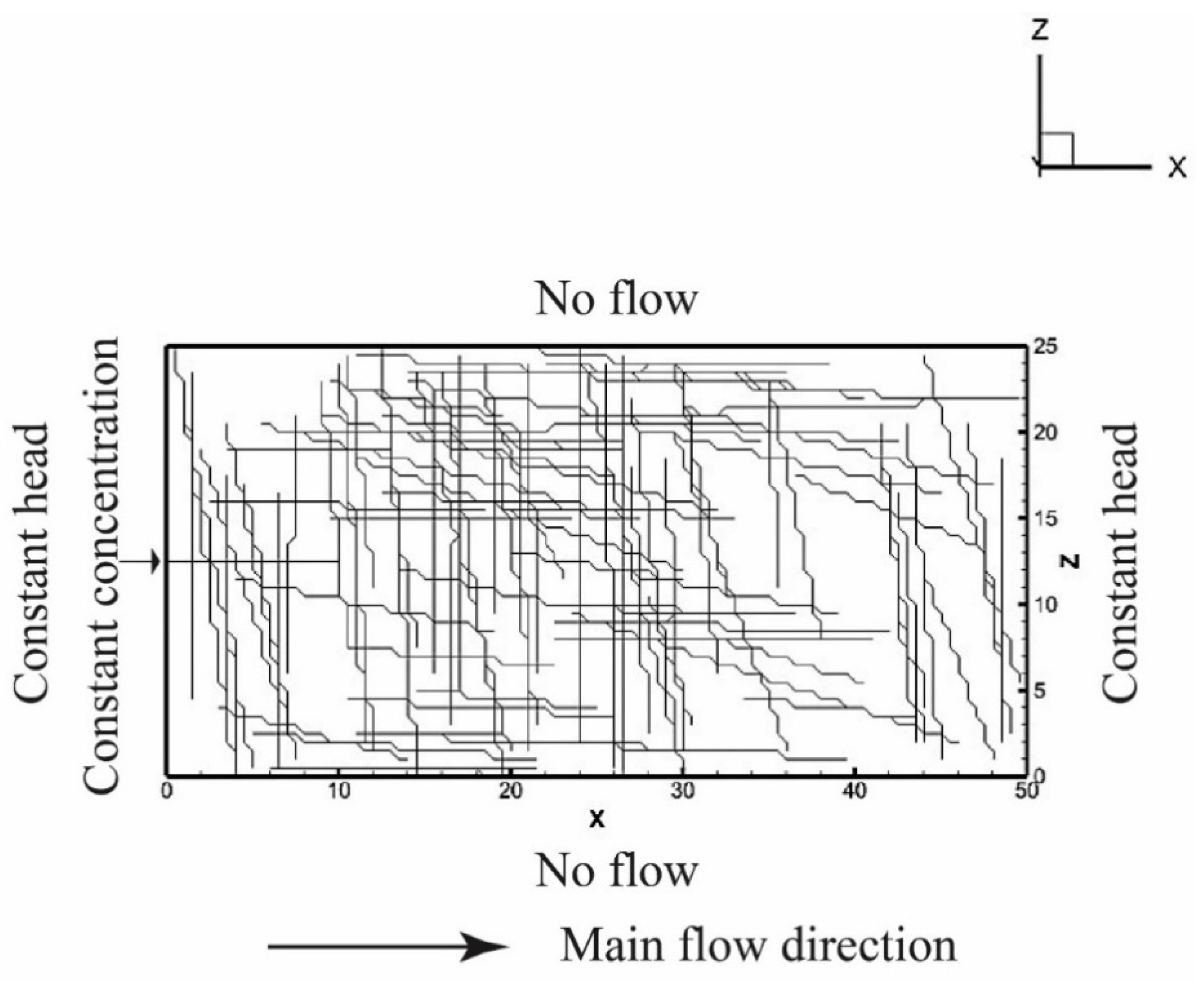
2.1. Generating the Random Discrete Fracture Networks

The model geometry, shown in Figure 1, is 50 × 25 m²_, and represents a horizontal, two-dimensional (2D) map view of the fractures, with unit thickness and uniform blocks (100 × 50) along the x and z axes. One hundred 2D DFN realizations (for each scenario) were generated by superimposing two different sets of fractures onto the grid, with links between the fracture elements and matrix block elements, leading to realistic DFNs [46,47]. Each scenario represented the ensemble average of 100 total individual DFN flow and transport realizations. Fracture locations, orientations, lengths, and hydraulic conductivities were generated from predefined distributions obtained in literature [32,48]:

(1)

Fracture location: distributed randomly over the entire domain, with a random seed selected for each realization;

(2)

Fracture orientation: two fracture sets followed mixed Gaussian distributions (each Gaussian distribution is equally weighted and has its own mean and variance), with a mean and standard deviation of 0° ± 10° for the first set, and 90° ± 10° for the second set;

(3)

Fracture length: log-normal distribution, with 10 length bins—the mean of the smallest length bin is 2.5 m (which is 1/10 of the minimum length of the x and z domain sizes), and the mean of the largest length bin is 25 m (which is the minimum length of the x and z domain sizes);

(4)

Fracture aperture: exponential distribution, with 10 aperture bins—the mean of the smallest aperture bin is 0.001 m, and the mean of the largest aperture bin is 0.0015 m.

Fracture permeability was calculated using the parallel plate law: k_f = ω_f²/12 [7,49,50,51], which relates aperture ω_f to permeability k_f. In our DFNs, fractures were open and act as flow conduits. Fracture permeability was dependent on aperture, and varied from 8.3 × 10⁻⁸ m² to 1.9 × 10⁻⁷ m² given an exponential distribution. We tested the matrix hydraulic conductivity of 5 × 10⁻⁸, 1 × 10⁻⁷ and 1 × 10⁻⁶ m/s, with the corresponding permeability of 5.5 × 10⁻¹⁵, 1.1 × 10⁻¹⁴ and 1.1 × 10⁻¹³ m², which are six to seven orders of magnitude smaller than the fracture permeability. The matrix permeability was assumed to be isotropic and in the range of an un-fractured, low-permeability rock, like a real silt medium ([1.15 × 10−16, 2.3 × 10−12] m²). One realization of the DFN, with 100 fractures, is shown in Figure 1. A horizontal fracture with the length of 10 m and aperture of 0.001 m was inserted into the middle of the left boundary, in order to inject a conservative tracer. This zone provided a mobile source of pollutant, representing real-world contamination, where a pollutant usually enters firstly the mobile region in aquifers before spreading downstream.

2.2. Modeling Groundwater Flow and Pollutant Transport through the Discrete Fracture Networks

Steady-state groundwater flow through the confined aquifer generated above was then solved by HGS. Parameters for the flow model, including the specific storage coefficient and porosity, are defined in

Table 1. Model parameters and initial and boundary conditions used in the simulations.

Parameter	Symbol	Value	Unit
Matrix	-	-	-
Hydraulic conductivity	Kxx = Kyy = Kzz	5 × 10−8, 10−7, 10−6	m·s−1
Specific storage	Ss	10−3	m−1
Porosity	θs	0.3	-
Longitudinal dispersivity	αL	0.01	m
Transverse dispersivity	αT	0.001	m
Vertical_transverse dispersivity	αV	0.001	m
Tortuosity	τ	1	-
Fractures	-	-	-
Conductivity (computed)	Kf	(ρgωf2)/(12μ) a	m·s−1
Specific storage (computed)	Ssf	ρgαω b = 4.3 × 10−6	m−1
Longitudinal dispersivity	αLf	0.01	m
Transverse dispersivity	αTf	0.001	m
Vertical_transverse dispersivity	αVf	0.001	m
Solute	-	-	-
Free-solution diffusion coefficient	Dfree	10−9	m2/s
Initial conditions	-	-	-
Concentration	Ct=0	0	kg/m3
Boundary conditions	-	-	-
Inflow concentration	Cx=0	1	kg/m3
Simulation Settings	-	-	-
Tracer pulse	Ttracer	10	s
a ωf stands for aperture; μ stands for fluid viscosity		-	-
b αω stands for fluid compressibility		-	-

. Boundary conditions were chosen so that the main flow direction was from left to right, with a general hydraulic gradient of approximately 0.2. The high hydraulic gradient was selected for faster convergence, and decreased simulation times in this work (so that we could observe the late-time behavior of solute transport, which is critical to identify the dynamics of sub-diffusive non-Fickian transport). The left and right boundaries were set to be constant head boundary conditions, and had values as 50 m and 40 m, respectively.

Pollutant transport through the saturated DFN was then solved by HGS, using the same ILU (Incomplete lower upper factorization)-preconditioned ORTHOMIN (an iterative method using orthogonalization and minimization to achieve fast convergence) solver as is used for the flow problem. Transport parameters are shown in Table 1. The longitudinal, transverse, and vertical transverse dispersivities assigned to both the un-fractured rock matrix and rock fractures were 0.01, 0.001, and 0.001 m, respectively, where the longitudinal dispersivity was one order of magnitude smaller than the grid size, and the horizontal dispersivity was one order of magnitude smaller than that along the longitudinal direction. Tortuosity was assumed to be 1, so that we could focus on the impact of other measurable parameters (such as matrix permeability and porosity) on transport behaviors. A 10 s pulse of one conservative solute, representing an example of sodium chloride, with a nominal concentration of 1 kg/m³_, was injected into the fracture, explicitly inserted at the middle of the left boundary. The free solution diffusion coefficient was 1 × 10⁻⁹ m²/s (which is on the same order of the diffusion coefficient for hydrogen in water). The matrix porosity (0.30) was selected after referring to literature [52,53] where a value of 0.25–0.27 was assumed for the matrix porosity. We also tested a much smaller matrix porosity (0.05), and results (not shown here) revealed a tracer BTC (shifted toward younger times, likely due to a higher diffusion rate) with the overall trend similar to that with a porosity of 0.30.

The HGS transport time weighting factor was set to a fully implicit numerical scheme. Fully implicit time weighting is less prone to exhibit oscillations than central and explicit time weighting.

The governing equation for subsurface flow in porous media used in the HGS was a modified form of Richards’ equation [54]:

$$-\nabla •({\omega }_{m}q)+{\displaystyle \sum {\mathsf{\Gamma }}_{ex}\pm Q={\omega }_m\frac{\partial {\theta }_s}{\partial t}}$$

(1)

where ω_m [dimensionless] is the volumetric fraction of the total porosity occupied by the porous medium, Γ_ex [L³L⁻³T⁻¹] represents the volumetric fluid exchange rate between the subsurface domain and discrete fractures, Q [L³L⁻³T⁻¹] represents a source/sink term to the porous medium system, and θ_s [dimensionless] is the saturated water content which is assumed equal to the porosity. The fluid flux q [LT⁻¹] in (1) is given by Darcy’s law:

$$q=-K•k_r\nabla (\psi +z)$$

(2)

where K [LT⁻¹] is hydraulic conductivity tensor, k_r [dimensionless] represents the relative permeability of the medium, ψ [L] is the pressure head, and z [L] is the elevation head.

A fracture is idealized as the space between two-dimensional parallel surfaces, with the tacit assumption that the total head is uniform across the fracture width. The equation for saturated flow in a fracture of width/aperture ω_f [L] can be written by using the analogy of Richards Equation (1) for the porous matrix. The governing two-dimensional flow equation in a fracture has the form [44]:

$$-\overline{\stackrel{‾}{\nabla }}•({\omega }_f{q}_f)-{\omega }_f{\mathsf{\Gamma }}_f={\omega }_f{S}_{sf}\frac{\partial {\psi }_f}{\partial t}$$

(3)

where the fluid flux q_f [LT⁻¹] is given by:

$$q_f=-K_f•k_{rf}\overline{\stackrel{‾}{\nabla }}({\psi }_f+z_f)$$

(4)

where $\overline{\stackrel{‾}{\nabla }}$ is the two-dimensional gradient operator defined in the fracture plane, k_rf [dimensionless] is the permeability of the fracture, ψ_f and z_f [L] are the pressure and the elevation heads within the fracture, and S_sf [L⁻¹] is the specific storage coefficient for the fractures.

The saturated hydraulic conductivity of a fracture K_f [LT⁻¹] with a uniform aperture ω_f is given by: K_f = ρgω_f²/12μ. Because it was assumed that the fractures were non-deformable and fluid-filled, there was no contribution to the storage term from fracture compressibility. Thus, the specific storage coefficient for a fracture under saturated conditions was only related to the compressibility of water α_w [LT²M⁻¹], according to: S_sf = ρgα_w.

Three-dimensional transport of solutes in a saturated porous matrix is described by the following advection-dispersion equation [44]:

$$-\nabla •{\omega }_m(qC-{\theta }_{s}D\nabla C)+[{\omega }_m{\theta }_{s}R\lambda C]+{\displaystyle \sum {\mathsf{\Omega }}_{ex}\pm Q_c=}{\omega }_m[\frac{\partial ({\theta }_{s}RC)}{\partial t}+{\theta }_{s}R\lambda C]$$

(5)

where C is the solute concentration [ML⁻³], R [dimensionless] is the retardation factor, Ω_ex [ML⁻³T⁻¹] represents the mass exchange rate of solutes per unit volume between the subsurface domain and discrete fractures, and λ is a first-order decay constant [L⁻¹]. Solute exchange with the outside of the simulation domain is represented by Q_c [ML⁻³T⁻¹] which represents a source or a sink to the porous medium system.

The equation for solute transport in a saturated fracture is:

$$-\nabla •({\omega }_f{q}_f{C}_f-{\omega }_f{\theta }_f{D}_f\nabla C_f)+{\omega }_f[R_f{\lambda }_f{C}_f]-{\omega }_f{\mathsf{\Omega }}_f={\omega }_f[\frac{\partial ({\theta }_f{R}_f{C}_f)}{\partial t}+{\theta }_f{R}_f{\lambda }_f{C}_f]$$

(6)

where C_f is the concentration in a fracture [ML⁻³], λ_f is a first-order decay constant [L⁻¹], D_f is the hydrodynamic dispersion tensor of the fracture [L²T⁻¹], and R_f [dimensionless] represents retardation factor.

2.3. Applying the Fractional Advection–Dispersion Equations to Quantify Transport

If the solute is initially placed in the mobile zone (i.e., a fracture along the main flow direction), the corresponding fADE takes the form [55]:

$$\frac{\partial C_m}{\partial t}+\beta \frac{{\partial }^{\gamma }{C}_m}{\partial t^{\gamma }}=-\nabla \cdot \left[v{C}_m-D\nabla C_m\right]-\beta C_m(x,t=0)\frac{t^{-\gamma }}{\mathsf{\Gamma }(1-\gamma )}$$

(7)

$$\frac{\partial C_{im}}{\partial t}+\beta \frac{{\partial }^{\gamma }{C}_{im}}{\partial t^{\gamma }}=-\nabla \cdot \left[v{C}_{im}-D\nabla C_{im}\right]+C_m(x,t=0)\frac{t^{-\gamma }}{\mathsf{\Gamma }(1-\gamma )}$$

(8)

where C_m and C_im [ML⁻³] denote the solute concentration in the mobile and immobile phases, respectively; γ [dimensionless] (0 < γ ≤ 1) is the time index; β [T^γ−1] is the fractional-order capacity coefficient; v [LT⁻¹] and D [L²T⁻¹] are the effective velocity and dispersion coefficient, respectively; and Γ(·) is the Gamma function.

Meerschaert et al. [56] generalized the fADE (7) and (8) by introducing an exponentially-truncated power-law function, which is an incomplete gamma function, as the memory function:

$$g(t)={\displaystyle {\int }_t^{\infty }{e}^{-\lambda s}\frac{\gamma s^{-\gamma -1}}{\mathsf{\Gamma }(1-\gamma )}}ds$$

(9)

where λ > 0 [T⁻¹] is the truncation parameter in time. This modification leads to the tempered time fADE (tt-fADE) [56,57]:

$$\frac{\partial C_m}{\partial t}+\beta e^{-\lambda t}\frac{{\partial }^{\gamma }}{\partial t^{\gamma }}\left[e^{\lambda t}{C}_m\right]-\beta {\lambda }^{\gamma }{C}_m=-\nabla \cdot \left[v{C}_m-D\nabla C_m\right]-\beta C_m^0{\displaystyle {\int }_t^{\infty }{e}^{-\lambda \tau }}\frac{{\tau }^{-\gamma -1}}{\mathsf{\Gamma }(1-\gamma )}d\tau$$

(10)

$$\frac{\partial C_{im}}{\partial t}+\beta e^{-\lambda t}\frac{{\partial }^{\gamma }}{\partial t^{\gamma }}\left[e^{\lambda t}{C}_{im}\right]-\beta {\lambda }^{\gamma }{C}_{im}=-\nabla \cdot \left[v{C}_{im}-D\nabla C_{im}\right]+C_m^0{\displaystyle {\int }_t^{\infty }{e}^{-\lambda \tau }}\frac{{\tau }^{-\gamma -1}}{\mathsf{\Gamma }(1-\gamma )}d\tau$$

(11)

where $C_m^0=C_m\left(x,t=0\right)$ denotes the initial source, located in the mobile phase or fractures. A few parameters in the tt-fADE (10) and (11) including the effective velocity v and the dispersion coefficient D, may be determined by field experiments (i.e., monitoring wells) and laboratory experiments (transport through fractured media), while the other parameters should be approximated given the plumes observed in the field. The poor predictability of the fADE model motivated us to explore the relationship between DFN properties and model parameters in Section 4.

At the late time

$$t<<1/\lambda$$

(12)

the tail of BTC for solutes in the mobile declines as a power-law function:

$$C_m(x,t)\propto t^{-1-\gamma }$$

(13)

The tail of the total-phase BTC also declines as a straight line in a log–log plot with a rate:

$$C(x,t)\propto t^{-\gamma }$$

(14)

while at a much later time $t>>1/\lambda$, the slope of the mobile/total-phase BTC reaches infinity (i.e., the late-time BTC tail declines exponentially). Therefore, the value of λ controls the transition of the BTC late-time tail from a power-law function to exponential function [57].

In the following sections, we try to link the time index γ to characteristics of the fractured porous media.

3. Results of Monte Carlo Simulations

The ensemble average of BTCs for all 100 realizations for each DFN scenario are shown in Figure 2, along with the best-fit solutions using the tt-fADE model (10) and (11). Three scenarios of DFN were considered, by setting the total number of fractures to 20, 60, and 80, and holding mean fracture set orientations constant to 0° and 90°. An additional fourth scenario explored the impact of fracture orientation on transport dynamics, by changing mean fracture set orientation to −45° and 45° for a 60 fracture DFN.

The best-fit parameters of the tt-fADE model (10) and (11) for all DFNs are listed in

Table 2. Best-fit parameters for the tt-fADE model (10) and (11) for discrete fracture networks (DFNs) with different fracture densities and orientation scenarios. In the legend, v denotes the effective velocity, D is the dispersion coefficient, γ is the time/scale index, β is the fractional-order capacity coefficient, λ is the truncation parameter, and S_BTC stands for the late-time BTC slope in a log–log plot.

Fracture Numbers	v [m/day]	D [m2/day]	β [dayγ−1]	γ [Dimensionless]	λ [day−1]	SBTC [Dimensionless]
20 (0°~90°)	0.46	9.40	2.17	0.885	3.29 × 10−10	−2.088
60 (0°~90°)	10.53	40.36	5.46	0.667	3.76 × 10−14	−1.712
80 (0°~90°)	12.11	93.84	27.66	0.827	1.75 × 10−8	−1.965
60 (−45°~45°)	20.72	29.37	14.75	0.673	3.24 × 10−8	−1.689

. The effective velocity v, dispersion coefficient D, and fractional-order capacity coefficient β increase with an increasing fracture density. It is also noteworthy that β has the units of fractional-order in time, which can be converted to a dimensionless capacity coefficient β₀ = β γ λ^γ−1 (where β₀ represents the long-term ratio of immobile versus mobile mass). The other two parameters, including the time index γ and the truncation parameter λ, first decrease and then increase as the number of fractures increases. This trend implies that the DFN domain containing 60 fractures might exhibit higher degree of heterogeneity, and therefore translate from non-Fickian to Fickian transport at a much later time, compared to the DFN with 20 or 80 fractures. When the matrix hydraulic conductivity is set to be 10⁻⁷ m/s, the BTCs are more sensitive to fracture density. For example, when the number of fractures is 20, the peak concentration appears at day 365, while the DFN with 60 (or 80) fractures has the peak BTC at day 50 (or day 100). The truncation parameter λ can be calculated by the reciprocal of the cutoff time, representing the transition time from non-Fickian to Fickian transport; however, in this study, the power-law portion of BTCs persisted and the transition time could not be identified directly.

4. Discussion

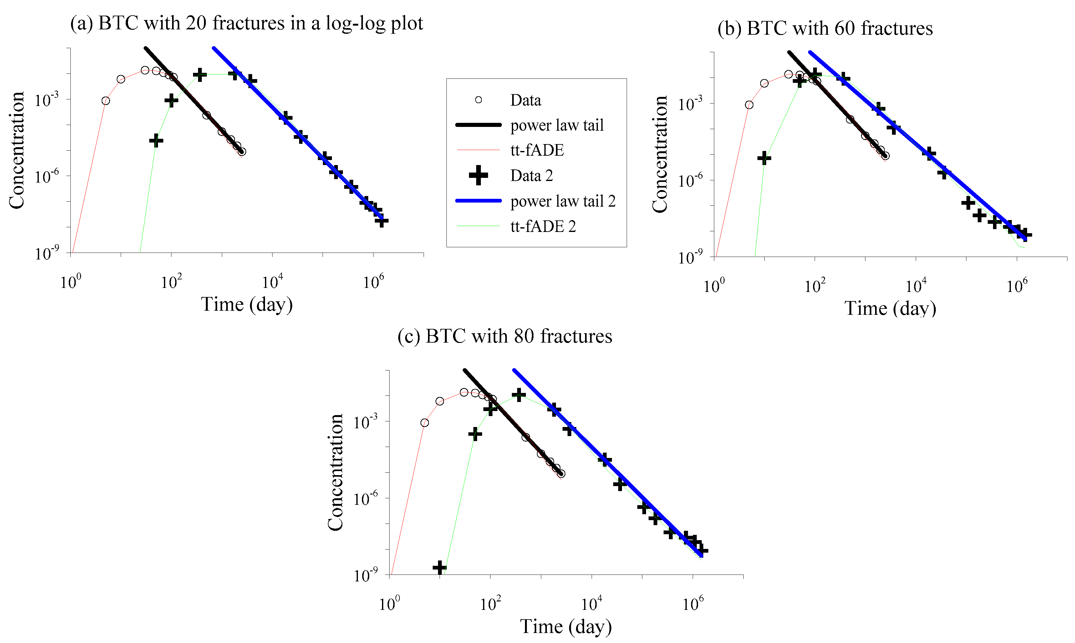
4.1. Impact of Fracture Density on Non-Fickian Transport

The simulations indicated that fracture density dominates non-Fickian transport dynamics, and therefore significantly affects tt-fADE model parameters. For example, a denser DFN contains more connected flow paths, leading to faster plume movement (i.e., a larger effective velocity v), greater plume spreading in space (corresponding to a larger dispersion coefficient D), and more fracture/matrix interaction (i.e., tracer particles have a higher probability of entering the surrounding matrix, which correlates to a larger value of the capacity coefficient β). In addition, the complex relationship between DFN density and other tt-fADE model parameters (time index γ and truncation parameter λ) can be explained by the hypothesis that moderately dense DFNs (i.e., fracture scenario with 60 fractures) maximize variations in matrix–fracture exchange rates, which leads to the heaviest late-time BTC tail (i.e., the smallest time index γ) and the persistent power-law BTC (i.e., the smallest truncation parameter λ). DFNs with a broader range of densities are needed in a future study to further investigate the above hypothesis.

The dominant impact of fracture density on pollutant transport may be due to two reasons. First, the number of fractures significantly affects the architecture of DFNs, including both the interconnectivity of fractures and the thickness of surrounding matrix. It is well-known that the interconnected fracture network forms the preferred flow paths in the formation [22,58,59]. These pathways are “paths of least resistance”, where most of the flow and solute is concentrated [7,26,36,60], resulting in early arrivals. Matrix block size, which is typically characterized using fracture spacing, affects trapping time and influences late-time tailing in BTCs. Second, networks containing higher fracture densities may yield a broader distribution of apertures [61], resulting in a larger variation of advective velocities in the system. Flow in the fracture is constrained to the two-dimensional domain of the fracture aperture, where average flux at any location within a fracture is proportional to the cube of the aperture [35,50,62]. Small variations in the aperture (which is 1 × 10³~1.5 × 10³ μm in this study), therefore, can cause large, non-linear variations in advective velocity.

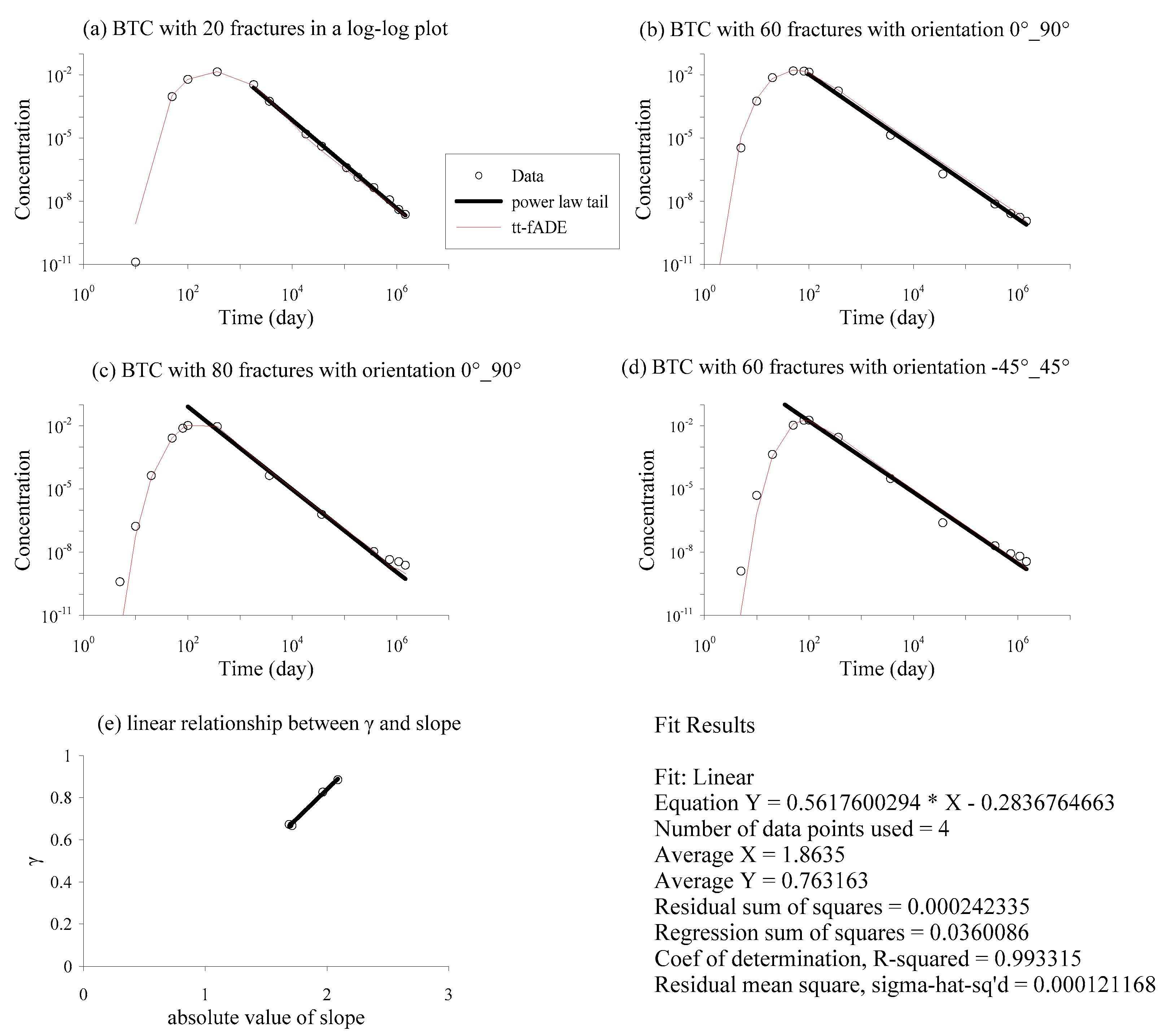
4.2. Impact of Fracture Orientation on Non-Fickian Transport

Fracture orientation has a complex impact on pollutant transport behavior. The DFN with mean fracture set orientations of −45° and 45° (where the overall flow direction is along 0°) provides two major directions for pollutant particles to move, while the DFN with mean fracture set orientations of 0° and 90° offers horizontally dominant motion for pollutants. Hence, the former has a relatively larger effective velocity and less spatial spreading (i.e., a smaller dispersion coefficient). Mean fracture set orientations of −45° and 45° also enhance the movement of solute particles into matrix blocks, resulting in a greater immobile mass (and hence a larger capacity coefficient β) than that for the cases with mean fracture set orientations of 0° and 90°. It is noteworthy, however, that the BTC peak occurs at a time determined by both the effective velocity v and the capacity coefficient β. The larger for v and/or the smaller for β, the earlier for the BTC peak. Although the DFNs with mean fracture orientations of −45° and 45° have a relatively larger v, the ensemble BTC peak appears later (at day 100) than that for the DFNs with mean fracture orientations of 0° and 90° (BTC peak occurs at day 50), because the DFNs with mean fracture orientations of −45° and 45° have a much larger β, which acts as part of the retardation coefficient (1 + β) when γ = 1. The DFNs with mean fracture orientations of −45° and 45° might also produce more tortuous pathways, which lead to greater transverse dispersion than the DFNs with mean fracture orientations of 0° and 90° [19]. Finally, regardless of fracture orientation, late-time BTCs exhibit similar slopes, and therefore the similar time index γ, if the DFNs have the same density and a constant distribution of fracture length. The latter impact (caused by the fracture length distribution), however, cannot be reliably investigated in this study, due to the field-scale DFNs (with a relatively small domain size). In a future study, we will increase the model domain size (to regional scale) and systematically explore the impact of fracture length distributions on non-Fickian dynamics.

The above analysis implies that the fracture density is more important than the fracture orientation in affecting the power-law late-time tailing of the BTC, while both properties can affect the plume mean displacement (captured mainly by the velocity in the tt-fADE model (10) and (11)), plume spreading (captured by the dispersion coefficient in model (10) and (11)), and fracture-matrix mass exchange ratio (captured by the capacity coefficient in (10) and (11)).

4.3. Impact of Matrix Permeability on Late-Time BTC

Rock matrix permeability may affect the late-time behavior of chemical transport. To explore this potential impact, here we conducted additional Monte Carlo simulations using different matrix permeability: (1) increasing matrix permeability by 10 times (from 1.1 × 10⁻¹⁴ m² to 1.1 × 10⁻¹³ m²) and (2) decreasing matrix permeability by 2 times (from 1.1 × 10⁻¹⁴ m² to 5.5 × 10⁻¹⁵ m²). Results are shown in Figure 3. We did not select the smaller value for matrix permeability, because preliminary numerical tests showed that if matrix permeability was smaller than 1.1 × 10⁻¹⁵ m², the numerical iteration (in the flow model) could not converge.

The BTC declines faster at the late time with an increasing matrix permeability. This is because the matrix domain with higher permeability leads to shorter trapping times for chemical particles. Contrarily, the average velocity is smaller for a rock matrix with smaller permeability, resulting in heavier late-time tailing in the BTC.

4.4. How to Approximate the Time Index γ Given the Limited Late-Time BTC

Although the transport time considered by our Monte Carlo simulation is very long (about 5000 years), we could not observe the transition in the BTC from persistent non-Fickian to Fickian transport behaviors (in the Monte Carlo simulations performed in this study, the total modeling time could not be longer than 2 × 10⁶ days, since the concentration at the outlet after 2 × 10⁶ days is so small that HGS generates negative BTCs). It is common that the measured BTC cannot last long enough to cover the whole power-law portion and its transition in the BTC at late times, due to the usually limited sampling period, as well as the low concentration at the late time, which might be below the detection limit. The time index γ cannot be directly estimated when the power-law portion of the BTC at the late time cannot be identified.

One possible way to solve the above challenge is to approximate γ using the BTC’s recession limb. In this study, the recession limb of each measured BTC exhibits a straight line in a log–log plot (Figure 2), which indicates prolonged non-Fickian or anomalous transport. There is a linear relationship between the slope of the BTC recession limb (whose absolute value is denoted as |S_BTC|) and the time index γ in the tt-fADE model (10) and (11):

γ = 0.5618 × |S_BTC| − 0.2837

(15)

where the corresponding coefficient of determination is 0.9933 (i.e., strong correlation). Since |S_BTC| can be measured easily (here “easily” means that one can use the observed BTC, shown for example in Figure 2, to directly obtain the slope of the BTC, which is the negative value of |S_BTC|), the above linear relationship might be practically useful. However, this approximation will be ineffective if the power-law portion of the BTC is too short to observe (which represents a fast transfer from non-Fickian to Fickian diffusion), or the data contains apparent noises (which can be common for the measurement of low concentrations at the BTC tails in the field).

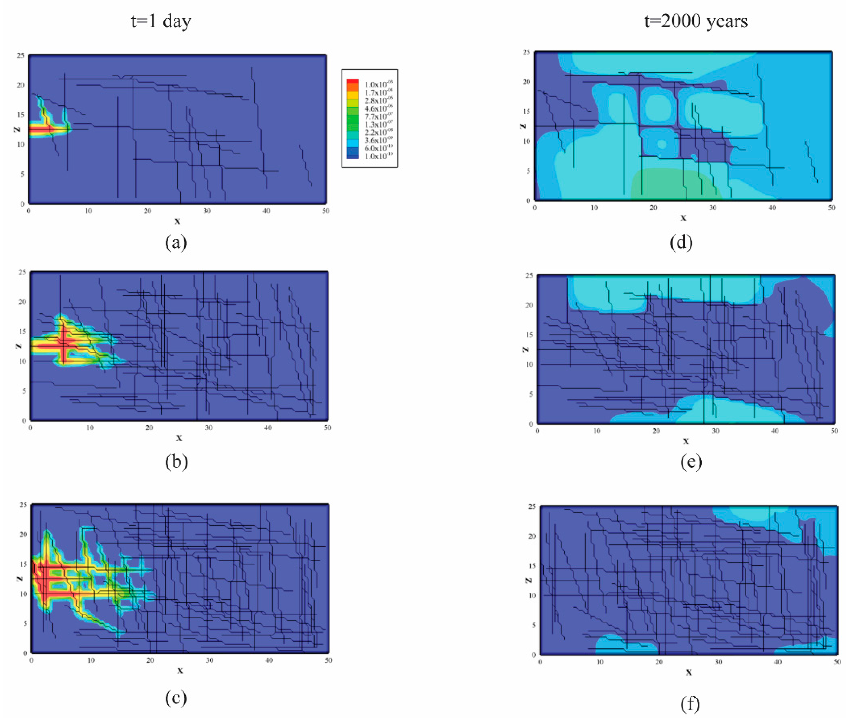
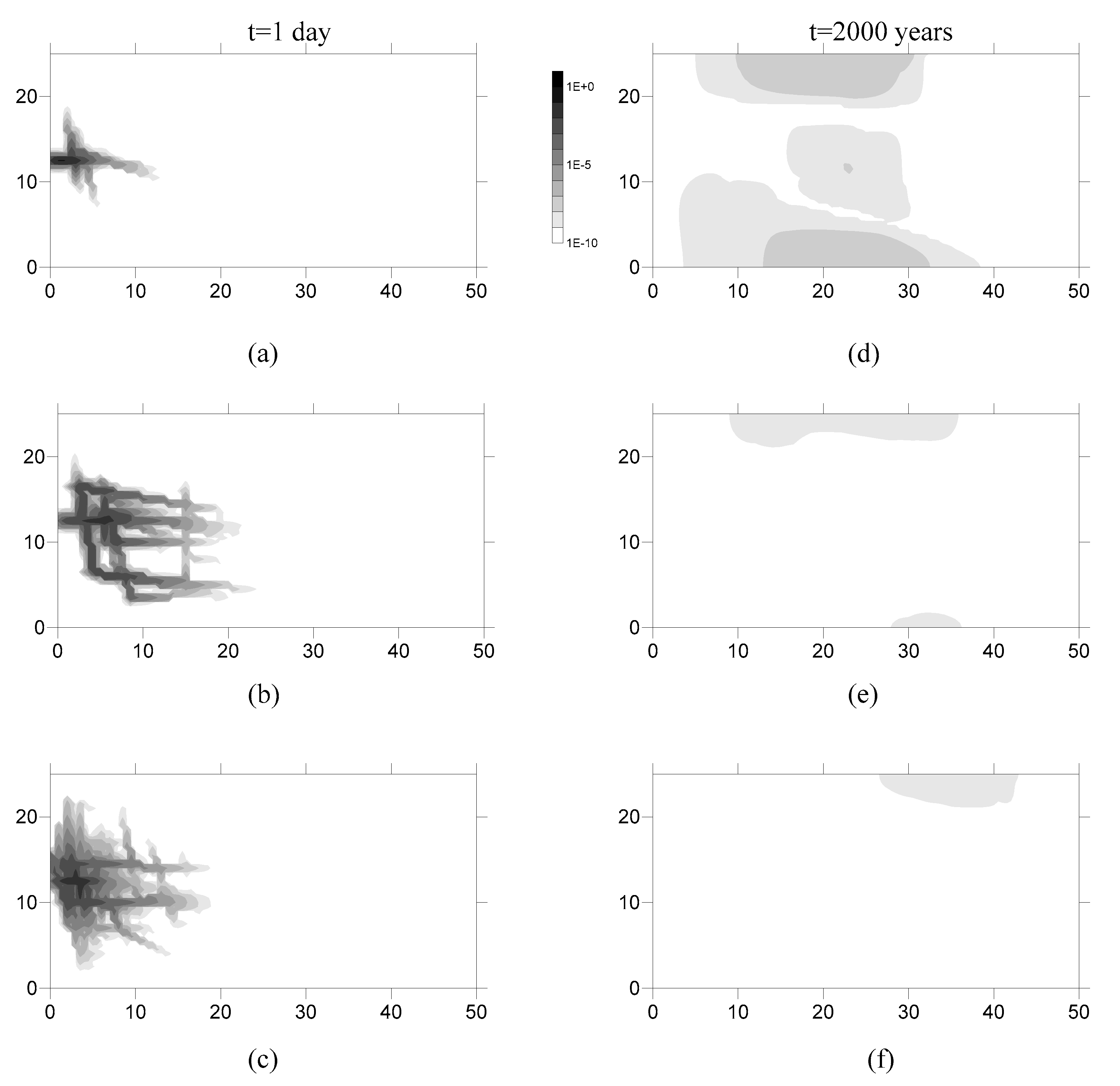
4.5. Subdiffusive Transport Shown by Plume Snapshots

We further explored the spatial distribution of a chemical in the DFNs, by depicting plume snapshots at different times for a single realization, and the ensemble average of the Monte Carlo results (Figure 4 and Figure 5).

We chose the first time step (t = 1 day) to show the early arrivals for the three different fracture densities with matrix permeability of 1.1 × 10⁻¹⁴ m². All the three cases show that chemical particles move along the preferential flow paths. With increasing fractures in the DFNs, the plume spreads to a wider area in the vertical direction with a more uniform moving front. For the 13th time step (t = 2000 years), the snapshots exhibited apparent retention and sequestration (meaning that the surrounding low-permeable matrix trapped chemical particles, especially near the source [39,63]) in the least-dense fractured network. Competition between channeling and sequestration leads to persistent non-Fickian dynamics. Fast- and slow-moving chemical particles are counterbalanced, and the effective velocity becomes larger for the DFNs with more fractures.

5. Conclusions

This study aims to explore the relationship between real-world aquifer properties and non-Fickian transport dynamics, so that the fractional partial differential equations built upon fractional calculus can be reliably applied with appropriate hydrogeologic interpretations. We use the Monte Carlo approach to generate field-scale DFNs where the fracture properties change systematically, and then to simulate groundwater flow and pollutant transport through the complex DFNs. For a point source located initially in the mobile phase or fracture, the late-time behavior for the BTCs simulated by the Monte Carlo approach is then explained by the tempered–stable time fractional advection–dispersion equation. We build the relationship between medium heterogeneity and transport dynamics through the combination of numerical experiments and stochastic analysis. The following five primary conclusions were found.

First, the DFN density is the major factor affecting non-Fickian transport at the late time, since (1) the number of fractures significantly affects the internal structure of DFNs; and (2) DFNs containing a higher fracture density may yield broader distribution of apertures, resulting in greater variation of advective velocities. A moderate dense DFN (filled with 60 fractures) results in the most heterogenous domain and the heaviest late-time tail in the BTCs, implying that there might exist a potential threshold of fracture density for non-Fickian dynamics when both the domain size and the fracture length distribution remain unchanged.

Second, for the DFNs with the same density and different mean orientations, the late time tailing behavior is affected by the ratio of fractures along different directions. More longitudinal fractures aligned with the overall flow direction will lead to an increase in earlier arrivals, while more transverse fractures, with flow deviating from the general flow direction, will enhance chemical particles to interact with the rock matrix, resulting in a greater immobile mass (a larger β in the tt-fADE) and a heavier late-time tailing. The BTC peak time is determined by both the effective velocity and capacity coefficient β (representing the immobile mass ratio). The time index and the slope of the late-time BTC, however, are similar for the DFNs with the similar density and different mean orientations, since the fracture density dominates the distribution of the mass exchange rate between fracture and matrix (and therefore defines the index of the time fractional derivative in the tt-fADE model).

Third, a rock matrix with higher permeability will lead to a relatively more homogeneous domain with a larger time index and a steeper slope in the late-time BTC, since the trapping times in rock matrix becomes relatively shorter.

Fourth, the DFN properties can be quantitatively linked to the slope of the recession limb of the BTC. Particularly, the time index γ in the tt-fADE model has a simple, linear empirical expression with the power-law slope of the BTC recession limb, which can help estimate the index γ in practical applications where the chemical transport time is usually not long enough to cover the full range of late-time transport behavior.

Fifth, plume snapshots show that all the three fracture densities built in this study exhibit early arrivals and sequestration effects. The denser DFNs can produce more early arrivals, due to more preferential flow paths, while the sparse DFNs tend to show heavier sequestration near the source. Therefore, competition between the channeling effect (in relative high-permeable fractures or the mobile phase) and the trapping effect (in the surrounding rock matrix or immobile domains) results in complex prolonged non-Fickian characteristics in chemical transport. With predictable parameters, the fractional partial differential equations can be used as an efficient upscaling tool to address real-world contamination problems.

References

1. Gorenflo, R.; Mainardi, F. Fractional Calculus. In Fractals and Fractional Calculus in Continuum Mechanics; Mainardi, F., Ed.; Springer: Vienna, Austria, 1997; pp. 223–276. [Google Scholar]
2. Metzler, R.; Klafter, J. The random walk’s guide to anomalous diffusion: A fractional dynamics approach. Phys. Rep. 2000, 339, 1–77. [Google Scholar] [CrossRef]
3. Zhang, Y.; Sun, H.G.; Stowell, H.H.; Zayernouri, M.; Hansen, S.E. A review of applications of fractional calculus in Earth system dynamics. Chaos Solitons Fractals 2017, 102, 29–46. [Google Scholar] [CrossRef]
4. Fogg, G.E.; Zhang, Y. Debates—Stochastic subsurface hydrology from theory to practice: A geologic perspective. Water Resour. Res. 2016, 52, 9235–9245. [Google Scholar] [CrossRef]
5. Coats, K.H.; Smith, B.D.; van Genuchten, M.T.; Wierenga, P.J. Dead-End Pore Volume and Dispersion in Porous Media. Soil Sci. Soc. Am. J. 1964, 4, 73–84. [Google Scholar] [CrossRef]
6. Haggerty, R.; McKenna, S.; Meigs, L.C. On the late-time behaviour of tracer breakthrough curves. Water Resour. Res. 2000, 36, 3467–3479. [Google Scholar] [CrossRef]
7. Klepikova, M.V.; Le Borgne, T.; Bour, O.; Dentz, M.; Hochreutener, R.; Lavenant, N. Heat as a tracer for understanding transport processes in fractured media: Theory and field assessment from multiscale thermal push-pull tracer tests. Water Resour. Res. 2016, 52, 5442–5457. [Google Scholar] [CrossRef] [Green Version]
8. Becker, M.W.; Shapiro, A.M. Tracer transport in fractured crystalline rock: Evidence of nondiffusive breakthrough tailing. Water Resour. Res. 2000, 36, 1677–1686. [Google Scholar] [CrossRef]
9. Kang, P.K.; Le Borgne, T.; Dentz, M.; Bour, O.; Juanes, R. Impact of velocity correlation and distribution on transport in fractured media: Field evidence and theoretical model. Water Resour. Res. 2015, 51, 940–959. [Google Scholar] [CrossRef] [Green Version]
10. Becker, M.W.; Shapiro, A.M. Interpreting tracer breakthrough tailing from different forced-gradient tracer experiment configurations in fractured bedrock. Water Resour. Res. 2003, 39. [Google Scholar] [CrossRef]
11. Benson, D.A.; Wheatcraft, S.W.; Meerschaert, M.M. Application of a fractional advection-dispersion equation. Water Resour. Res. 2000, 36, 1403–1412. [Google Scholar] [CrossRef]
12. Chang, F.X.; Chen, J.; Huang, W. Anomalous diffusion and fractional advection-diffusion equation. Acta Phys. Sin. 2005, 54, 1113–1117. [Google Scholar]
13. Huang, G.; Huang, Q.; Zhan, H. Evidence of one-dimensional scale-dependent fractional advection-dispersion. J. Contam. Hydrol. 2006, 85, 53–71. [Google Scholar] [CrossRef] [PubMed]
14. Green, C.T.; Zhang, Y.; Jurgens, B.C.; Starn, J.J.; Landon, M.K. Accuracy of travel time distribution (TTD) models as affected by TTD complexity, observation errors, and model and tracer selection. Water Resour. Res. 2014, 50, 6191–6213. [Google Scholar] [CrossRef]
15. Garrard, R.M.; Zhang, Y.; Wei, S.; Sun, H.; Qian, J. Can a Time Fractional-Derivative Model Capture Scale-Dependent Dispersion in Saturated Soils? Groundwater 2017, 55, 857–870. [Google Scholar] [CrossRef] [PubMed]
16. Schumer, R.; Meerschaert, M.M.; Baeumer, B. Fractional advection-dispersion equations for modeling transport at the Earth surface. J. Geophys. Res. Earth Surf. 2009, 114, 1–15. [Google Scholar] [CrossRef]
17. Drummond, J.D.; Aubeneau, A.F.; Packman, A.I. Stochastic modeling of fine particulate organic carbon dynamics in rivers. Water Resour. Res. 2014, 50, 4341–4356. [Google Scholar] [CrossRef]
18. Sun, H.G.; Chen, D.; Zhang, Y.; Chen, L. Understanding partial bed-load transport: Experiments and stochastic model analysis. J. Hydrol. 2015, 521, 196–204. [Google Scholar] [CrossRef]
19. Reeves, D.M.; Benson, D.A.; Meerschaert, M.M.; Scheffler, H.P. Transport of conservative solutes in simulated fracture networks: 2. Ensemble solute transport and the correspondence to operator-stable limit distributions. Water Resour. Res. 2008, 44, 1–20. [Google Scholar] [CrossRef]
20. Zhang, Y.; Baeumer, B.; Reeves, D.M. A tempered multiscaling stable model to simulate transport in regional-scale fractured media. Geophys. Res. Lett. 2010, 37, 1–5. [Google Scholar] [CrossRef]
21. Berkowitz, B. Characterizing flow and transport in fractured geological media: A review. Adv. Water Resour. 2002, 25, 861–884. [Google Scholar] [CrossRef]
22. Neuman, S.P. Trends, prospects and challenges in quantifying flow and transport through fractured rocks. Hydrogeol. J. 2005, 13, 124–147. [Google Scholar] [CrossRef]
23. Zhao, Z.; Rutqvist, J.; Leung, C.; Hokr, M.; Liu, Q.; Neretnieks, I.; Hoch, A.; Havlíček, J.; Wang, Y.; Wang, Z.; et al. Impact of stress on solute transport in a fracture network: A comparison study. J. Rock Mech. Geotech. Eng. 2013, 5, 110–123. [Google Scholar] [CrossRef]
24. Zhao, Z.; Jing, L.; Neretnieks, I.; Moreno, L. Numerical modeling of stress effects on solute transport in fractured rocks. Comput. Geotech. 2011, 38, 113–126. [Google Scholar] [CrossRef]
25. Selroos, J.; Walker, D.D.; Ström, A.; Gylling, B.; Follin, S. Comparison of alternative modelling approaches for groundwater flow in fractured rock. J. Hydrol. 2002, 257, 174–188. [Google Scholar] [CrossRef]
26. Mukhopadhyay, S.; Cushman, J.H. Monte Carlo Simulation of Contaminant Transport: II. Morphological Disorder in Fracture Connectivity. Transp. Porous Media 1998, 31, 183–211. [Google Scholar] [CrossRef]
27. Outters, N. A Generic Study of Discrete Fracture Network Transport Properties Using FracMan/MAFIC; SKB-R-03-13; International Atomic Energy Agency (IAEA): Vienna, Austria, 2003. [Google Scholar]
28. Gustafson, G.; Fransson, Å. The use of the Pareto distribution for fracture transmissivity assessment. Hydrogeol. J. 2006, 14, 15–20. [Google Scholar] [CrossRef]
29. Liu, R.; Li, B.; Jiang, Y. A fractal model based on a new governing equation of fluid flow in fractures for characterizing hydraulic properties of rock fracture networks. Comput. Geotech. 2016, 75, 57–68. [Google Scholar] [CrossRef]
30. Zhang, Y.; Benson, D.A.; Meerschaert, M.M.; Labolle, E.M.; Scheffler, H.P. Random walk approximation of fractional-order multiscaling anomalous diffusion. Phys. Rev. E Stat. Nonlinear Soft Matter Phys. 2006, 74, 1–10. [Google Scholar] [CrossRef] [PubMed]
31. Cortis, A.; Birkholzer, J. Continuous time random walk analysis of solute transport in fractured porous media. Water Resour. Res. 2008, 44, 1–11. [Google Scholar] [CrossRef]
32. McKenna, S.A.; Meigs, L.C.; Haggerty, R. Tracer tests in a fractured dolomite: 3. Double porosity, multiple-rate mass transfer processes in convergent flow tracer tests. Water Resour. Res. 2001, 37, 1143–1154. [Google Scholar] [CrossRef]
33. Cook, P.G. A Guide to Regional Groundwater Flow in Fractured Rock Aquifers; CSIRO: Canberra, Australia, 2003; p. 107. [Google Scholar]
34. Bear, J. Dynamics of Fluids in Porous Media; Dover Publications: New York, NY, USA, 1972; ISBN 0-486-65675-6. [Google Scholar]
35. Painter, S.; Cvetkovic, V. Upscaling discrete fracture network simulations: An alternative to continuum transport models. Water Resour. Res. 2005, 41, 1–10. [Google Scholar] [CrossRef]
36. Lei, Q. Characterisation and Modelling of Natural Fracture Networks: Geometry, Geomechanics and Fluid Flow. Ph.D. Thesis, Imperial College London, London, UK, 2016. [Google Scholar]
37. Bakshevskaia, V.A.; Pozdniakov, S.P. Simulation of Hydraulic Heterogeneity and Upscaling Permeability and Dispersivity in Sandy-Clay Formations. Math. Geosci. 2016, 48, 45–64. [Google Scholar] [CrossRef]
38. Kang, P.K.; Dentz, M.; Le Borgne, T.; Juanes, R. Anomalous transport on regular fracture networks: Impact of conductivity heterogeneity and mixing at fracture intersections. Phys. Rev. E Stat. Nonlinear Soft Matter Phys. 2015, 92, 1–15. [Google Scholar] [CrossRef] [PubMed]
39. Zhang, Y.; Benson, D.A.; Baeumer, B. Predicting the tails of breakthrough curves in regional-scale alluvial systems. Ground Water 2007, 45, 473–484. [Google Scholar] [CrossRef] [PubMed]
40. Zhang, Y.; Benson, D.A.; LaBolle, E.M.; Reeves, D.M. Spatiotemporal Memory and Conditioning on Local Aquifer Properties; DOE/NV/0000939-01, Publication #45244; Desert Research Institute: Las Vegas, NV, USA, 2009; p. 64. [Google Scholar]
41. Kelly, J.F.; Bolster, D.; Meerschaert, M.M.; Drummond, J.D.; Packman, A.I. FracFit: A robust parameter estimation tool for fractional calculus models. Water Resour. Res. 2017, 53, 2559–2567. [Google Scholar] [CrossRef]
42. Cacas, M.C.; Ledoux, E.; de Marsily, G.; Tillie, B.; Barbreau, A.; Durand, E.; Feuga, B.; Peaudecerf, P. Modeling fracture flow with a stochastic discrete fracture network: Calibration and validation: 1. The flow model. Water Resour. Res. 1990, 26, 479–489. [Google Scholar] [CrossRef]
43. McClure, M.W.; Mark, W.; Horne, R.N. Discrete Fracture Network Modeling of Hydraulic Stimulation: Coupling Flow and Geomechanics; Springer: Berlin, Germany, 2013; ISBN 3319003836. [Google Scholar]
44. Therrien, R.; McLaren, R.G.; Sudicky, E.; Panday, S.M. HydroGeoSphere a Three-dimensional Numerical Model Describing Fully-integrated Subsurface and Surface Flow and Solute Transport; Groundwater Simulations Group, University of Waterloo: Waterloo, ON, Canada, 2010; p. 429. [Google Scholar]
45. Chakraborty, P.; Meerschaert, M.M.; Lim, C.Y. Parameter estimation for fractional transport: A particle-tracking approach. Water Resour. Res. 2009, 45. [Google Scholar] [CrossRef]
46. Geiger, S.; Cortis, A.; Birkholzer, J.T. Upscaling solute transport in naturally fractured porous media with the continuous time random walk method. Water Resour. Res. 2010, 46. [Google Scholar] [CrossRef]
47. Long, J.C.S.; Remer, J.S.; Wilson, C.R.; Witherspoon, P.A. Porous media equivalents for network of discontinuous fractures. Water Resour. Res. 1982, 18, 645–658. [Google Scholar] [CrossRef]
48. Fiori, A.; Becker, M.W. Power law breakthrough curve tailing in a fracture: The role of advection. J. Hydrol. 2015, 525, 706–710. [Google Scholar] [CrossRef]
49. Klimczak, C.; Schultz, R.A.; Parashar, R.; Reeves, D.M. Cubic law with aperture-length correlation: Implications for network scale fluid flow. Hydrogeol. J. 2010, 18, 851–862. [Google Scholar] [CrossRef]
50. Keller, A.A.; Roberts, P.V.; Blunt, M.J. Effect of fracture aperture variations on the dispersion of contaminants. Water Resour. Res. 1999, 35, 55–63. [Google Scholar] [CrossRef]
51. Zhao, Z.; Li, B.; Jiang, Y. Effects of fracture surface roughness on macroscopic fluid flow and solute transport in fracture networks. Rock Mech. Rock Eng. 2014, 47, 2279. [Google Scholar] [CrossRef]
52. Edery, Y.; Geiger, S.; Berkowitz, B. Structural controls on anomalous transport in fractured porous rock. Water Resour. Res. 2016, 52, 5634–5643. [Google Scholar] [CrossRef]
53. Callahan, T.J.; Reimus, P.W.; Bowman, R.S.; Haga, M.J. Using multiple experimental methods to determine fracture/matrix interactions and dispersion of nonreactive solutes in saturated volcanic tuff. Water Resour. Res. 2000, 36, 3547–3558. [Google Scholar] [CrossRef]
54. Therrien, R.; Sudicky, E. Three-dimensional analysis of variably-saturated flow and solute transport in discretely-fractured porous media. J. Contam. Hydrol. 1996, 23, 1–44. [Google Scholar] [CrossRef]
55. Schumer, R.; Benson, D.A.; Meerschaert, M.; Baeumer, B. Fractal mobile/immobile solute transport. Water Resour. Res. 2003, 39. [Google Scholar] [CrossRef]
56. Meerschaert, M.M.; Zhang, Y.; Baeumer, B. Tempered anomalous diffusion in heterogeneous systems. Geophys. Res. Lett. 2008, 35, 1–5. [Google Scholar] [CrossRef]
57. Zhang, Y.; Green, C.T.; Baeumer, B. Linking aquifer spatial properties and non-Fickian transport in mobile-immobile like alluvial settings. J. Hydrol. 2014, 512, 315–331. [Google Scholar] [CrossRef]
58. Moreno, L.; Tsang, C.F. Multiple-Peak Response to Tracer Injection Tests in Single Fractures: A Numerical Study. Water Resour. Res. 1991, 27, 2143–2150. [Google Scholar] [CrossRef]
59. Gerke, H.H. Preferential flow descriptions for structured soils. J. Plant Nutr. Soil Sci. 2006, 169, 382–400. [Google Scholar] [CrossRef]
60. Reeves, D.M.; Parashar, R.; Pohll, G.; Carroll, R.; Badger, T.; Willoughby, K. Practical guidelines for horizontal hillslope drainage networks in fractured rock. Eng. Geol. 2013, 163, 132–143. [Google Scholar] [CrossRef]
61. Neuman, S.P. Multiscale relationships between fracture length, aperture, density and permeability. Geophys. Res. Lett. 2008, 35, L22402. [Google Scholar] [CrossRef]
62. Hirthe, E.M.; Graf, T. Fracture network optimization for simulating 2D variable-density flow and transport. Adv. Water Resour. 2015, 83, 364–375. [Google Scholar] [CrossRef]
63. LaBolle, E.M.; Fogg, G.E. Role of Molecular Diffusion in Contaminant Migration and Recovery in an Alluvial Aquifer System. Transp. Porous Media 2001, 42, 155–179. [Google Scholar] [CrossRef]
Figure 1. Map of the fractured domain, showing flow geometry and boundary conditions. Note that the discrete fractures are curved in the figure, after they are incorporated into the grid by HydroGeoSphere (HGS).
Mathematics 06 00005 g001
Figure 2. Breakthrough curves (BTCs) at the control plane x = 50 m for three different fracture densities (ac); (b,d) have the same fracture density with different orientations. The BTC data (i.e., symbols) are simulated by HGS. The red line is the solution of the tempered time fADE (tt-fADE) model (10) and (11). The black line is a power law approximation to the late time decay in concentration. (e) shows the empirical linear relationship between the slope of the power-law decay in concentration and the time index γ in the tt-fADE model (10) and (11).
Mathematics 06 00005 g002
Figure 3. BTCs at the control plane x = 50 m for three different fracture densities (ac) with matrix permeability of 1.1 × 10⁻¹³ m2 (red lines and circles) and 5.5 × 10⁻¹⁵ m2 (green lines and crosses). The BTC data (i.e., symbols) are simulated by HGS. The red/green line is the solution of the tt-fADE model (10) and (11). The black/blue line is a power-law approximation to the late time decay in concentration.
Mathematics 06 00005 g003
Figure 4. One realization of plume snapshots for the first time step (t = 1 day) for the three different fracture densities: (a) the DFNs with 20 fractures; (b) 60 fractures; and (c) 80 fractures. The 13th time step (t = 2000 years) for the three different fracture densities: (d) 20 fractures; (e) 60 fractures; and (f) 80 fractures.
Mathematics 06 00005 g004
Figure 5. Monte Carlo results of plume snapshots for the first time step (t = 1 day) for the three different fracture densities: the DFNs with (a) 20 fractures; (b) 60 fractures and (c) 80 fractures. The 13th time step (t = 2000 years) for the three different fracture densities: (d) 20 fractures; (e) 60 fractures and (f) 80 fractures.
Mathematics 06 00005 g005