Lie Symmetries, Optimal System and Invariant Reductions to a Nonlinear Timoshenko System

Abstract

Lie symmetries and their Lie group transformations for a class of Timoshenko systems are presented. The class considered is the class of nonlinear Timoshenko systems of partial differential equations (PDEs). An optimal system of one-dimensional sub-algebras of the corresponding Lie algebra is derived. All possible invariant variables of the optimal system are obtained. The corresponding reduced systems of ordinary differential equations (ODEs) are also provided. All possible non-similar invariant conditions prescribed on invariant surfaces under symmetry transformations are given. As an application, explicit solutions of the system are given where the beam is hinged at one end and free at the other end.

1. Introduction

The problem of transverse vibration of beams is of importance in many engineering problems. Some of the early studies were based on the Euler–Bernoulli model, which takes into account the bending moment and the lateral displacement. Later models were based on adding shear or rotary inertia effect. In [1,2], Timoshenko proposed taking into consideration the shear, as well as the rotation effects, which proved to be suitable for non-slender beams and high frequency vibrations. Dimplekumar et al. [3] discuss the mathematical modeling for the mechanics of a solid using the distribution theory of Schwartz to the beam bending differential equations; the governing differential equations of a Timoshenko beam with jump discontinuities in slope, deflection, flexural stiffness and shear stiffness were obtained in this paper in the space of generalized functions. Mustafa and Messaoudi [4] and Fatiha [5] studied stability of the following Timoshenko system with the nonlinear frictional damping term in one equation:

$$\begin{array}{c}\hfill {\rho }_1{\phi }_{tt}-k{({\phi }_x+\psi )}_x=0,\\ \hfill {\rho }_2{\psi }_{tt}-EI{\psi }_{xx}+k({\phi }_x+\psi )+\chi ({\psi }_t)=0,\end{array}$$

(1)

where the functions $\phi$, $\psi$ depend on $(t,x)\in (0,\infty )\times (0,L)$ and model the vertical displacement of a beam and the rotation angle of a filament, respectively. The shear angle is $\psi -{\phi }_x$, and L denotes the length of the beam. The physical parameters appearing in the system are ${\rho }_1$, the mass density per unit length, ${\rho }_2$, the polar moment of inertia of a cross-section, E, Young’s modulus of elasticity, I, the moment of inertia of the cross-section, and k, the shear modulus. In this paper the beam is assumed to be uniform, that is the physical parameters ${\rho }_1,{\rho }_2,EI$ and k are all positive constants, and $\chi$ is an arbitrary nonlinear function of the damping term ${\psi }_t$.

We have solved this system by determining its symmetries and performing a Lie theoretic analysis as detailed below.

The classification of group invariant solutions of differential equations by means of the optimal systems is one of the main applications of Lie group analysis to differential equations. The main idea behind the method is discussed in detail in Ovsiannikov [6], Ibragimov [7], Olver [8] and Hydon [9]. We can always construct a family of group invariant solutions corresponding to a subgroup of a symmetry group admitted by a given differential equation. Since there is an infinite number of such subgroups, it is not possible to list all of the group invariant solutions. An effective and systematic way of classifying these group invariant solutions is to obtain optimal systems of subalgebras of the Lie symmetry algebra. This leads to non-similar invariant solutions under symmetry transformations.

Recall that one calls a list ${\left\{{\tilde{v}}_{\alpha }\right\}}_{\alpha \in \mathcal{A}}$ a one-dimensional optimal system, if it satisfies the conditions: (1) completeness, i.e., any one-dimensional subalgebra is equivalent to some ${\tilde{v}}_{\alpha }$; (2) inequivalence, i.e., ${\tilde{v}}_{\alpha }$ and ${\tilde{v}}_{\beta }$ are inequivalent for distinct $\alpha$ and $\beta$. In this paper, we have used all of the basic invariants to determine the conjugacy classes of one-dimensional subalgebras and at the same time shown that these representatives are comprehensive and mutually inequivalent. This is done by using the formula given in Section 3 of [10]. This formula is more or less a direct consequence of definitions. For the convenience of the reader, a detailed explanation is given in Section 2. The idea of using invariant functions to determine conjugacy classes is also discussed in [11,12].

Here is a brief outline of the paper. In Section 2, a formula for computing invariants in the adjoint representation is given. In Section 3, Lie symmetries and their Lie group transformations for the Timoshenko system are presented. In Section 4, an optimal system of one-dimensional subalgebras of the corresponding Lie algebra is derived. In Section 5, all possible invariant variables of the optimal system are presented; moreover, the corresponding reduced systems of ordinary differential equations (ODEs) are also given. As an illustration, some invariant solutions are given explicitly by solving the reduced systems of ODEs. Furthermore, all possible non-similar invariant conditions prescribed on invariant surfaces under symmetry transformations are given. A hinged-free beam has been considered in Example 1, with a constant torque control at the hinged end and a linear force control at the free end.

2. Invariants in the Adjoint Representations

The following formula is stated without a proof in [10]. Let $X_1,\dots ,X_N$ be a basis of the Lie algebra $\mathcal{L}$ and ${\omega }_1,\dots ,{\omega }_N$ be the corresponding dual basis of ${\mathcal{L}}^{*}$. Let X be an element of $\mathcal{L}$ and $Y={\sum }_{i=1}^N{x}_i{X}_i$ be a general element of $\mathcal{L}$. Then, $X_{\mathcal{L}}$, the fundamental vector field corresponding to X in the adjoint representation, is given by:

$$X_{\mathcal{L}}(Y)=\sum _{1\le i,j\le N}{x}_i{\omega }_j([X,X_i])\frac{\partial }{\partial x_j}.$$

To see this, recall that a vector field V on an open set $\Omega$ of ${\mathbb{R}}^N$ assigns to each point p of $\Omega$ a vector $V(p)=(V_1(p),\dots ,V_N(p))$. Therefore, if $e_1,\dots ,e_N$ is a basis of ${\mathbb{R}}^N$ and ${\omega }_1,\dots ,{\omega }_N$ is the dual basis, then:

$$V(p)=\sum _{i=1}^N{\omega }_i(V(p))e_i.$$

The vector field V gives rise to the differential operator of taking the directional derivative of any function f in the direction of $V(p)$. We identify V with the operator ${\sum }_{j=1}^N{\omega }_j(V(p))\frac{\partial }{\partial x_j}{\mid }_p.$

Specializing to the adjoint representation, the fundamental vector field $X_{\mathcal{L}}$ is given by:

$$X_{\mathcal{L}}(Y)=\frac{\partial }{\partial t}{\mid }_{t=0}{e}^{tadX}(Y)=[X,Y].$$

Therefore, if $Y={\sum }_{i=1}^N{x}_i{X}_i$ then:

$$X_{\mathcal{L}}(Y)=\sum _{1\le i,j\le N}{x}_i{w}_j([X,X_i])X_j=\sum _{1\le i,j\le N}{x}_i{w}_j([X,X_i])\frac{\partial }{\partial x_j}.$$

Application to Computations of Invariants

Let f be a function on $\mathcal{L}$, which is invariant in the adjoint representation of $\mathcal{L}$. This means that $f(expadtX)(Y)=f(Y)$ for all X in the Lie algebra $\mathcal{L}$ and all reals t. Therefore, if we write $f(x_1{X}_1+\dots +x_n{X}_n)=f(x_1,\dots ,x_n)$, then ${\sum }_{1\le i,j\le N}{x}_i{\omega }_j([X,X_i])\frac{\partial }{\partial x_j}f=0$. Letting X run through the basis $\{X_1,\dots ,X_N\}$, we get the system:

$$\begin{array}{cc}\sum _{1\le i,j\le N}{x}_i{\omega }_j([X_k,X_i])\frac{\partial f}{\partial x_j}=0,& k=1,\dots ,N.\end{array}$$

(2)

System (2) needs to be solved only for a set of generators of the Lie algebra $\mathcal{L}$. The solution of this linear system of partial differential equations (PDEs) gives the invariants in the adjoint representations.

For a solvable Lie algebra $\mathcal{L}$, it is best to work with the central series for the commutator ${\mathcal{L}}^{\prime }$ of $\mathcal{L}$, which is a nilpotent subalgebra. Therefore, one can find a chain of subalgebras, each an ideal in its successor and each of codimension one. Using this chain, one is essentially dealing with invariants of a single vector field, namely if we have found the basic invariants for a subalgebras S, which is an ideal of codimension one in $\tilde{S}$, then $\tilde{S}∕S$ operates on invariants of S, and this gives the invariants of $\tilde{S}$. Having obtained the invariants of ${\mathcal{L}}^{\prime }$, one can again reach $\mathcal{L}$ by a series of ideals, each of codimension one, to determine the basic invariants of $\mathcal{L}$. Such a series also gives a factorization of the group $G=⟨exp(AdX):X\in \mathcal{L}⟩$ in terms of one-dimensional subgroups.

The advantage of working with invariant functions is that if f is an invariant of $\mathcal{L}$ in the adjoint representation, then the adjoint group operates on the level sets, as well as sub-level sets of f, and one can systematically use invariants to work on level and sub-level sets of low dimensions to determine all of the conjugacy classes of one-dimensional subalgebras. This procedure will be used in Section 4 to determine one-dimensional optimal systems of the nonlinear damped Timoshenko system. This in turn will be used in Section 5 to determine optimal reduction.

3. Lie’s Infinitesimal Method

Lie symmetry method [13,14], described extensively in the literature, is invoked in the sequel to apply Lie symmetry analysis for Timoshenko System (1).

Using the invariance condition of the system of PDEs (1):

$$\begin{array}{c}{X}^{\left[2\right]}\left({\rho }_1{\phi }_{tt}-k{({\phi }_x+\psi )}_x\right){|}_{(1)}=0,\hfill \\ X^{\left[2\right]}\left({\rho }_2{\psi }_{tt}-EI{\psi }_{xx}+k({\phi }_x+\psi )+\chi ({\psi }_t)\right){|}_{(1)}=0,\hfill \end{array}$$

(3)

where $X^{\left[2\right]}$ is the second prolongation of the vector field differential operator:

$$X={\xi }^1\frac{\partial }{\partial t}+{\xi }^2\frac{\partial }{\partial x}+{\eta }^1\frac{\partial }{\partial \phi }+{\eta }^2\frac{\partial }{\partial \psi }.$$

Comparing coefficients of the various derivatives of the dependent variables $\phi$ and $\psi$ yields an over-determined linear PDE system. Carrying out the Janet basis of this over-determined system in the degree reverse lexicographical ordering as $\psi >\phi >x>t$ and ${\eta }_2>{\eta }_1>{\xi }_2>{\xi }_1$ by using the command “JanetBasis” involved in the Maple package “Janet” [15] leads to the following determining equations:

$$\begin{array}{c}[{\eta }_{\psi }^1,{\xi }_{\psi }^2,{\xi }_{\psi }^1,{\eta }_{\phi }^2,{\eta }_{\phi }^1-{\eta }_{\psi }^2,{\xi }_{\phi }^2,{\xi }_{\phi }^1,{\xi }_x^2,{\xi }_x^1,{\xi }_t^2,{\xi }_t^1,{\eta }_{\psi ,\psi }^2,{\eta }_{\psi ,x}^2,{\eta }_{\psi ,t}^2,{\eta }_{\psi ,t}^1,{\eta }_{\phi ,x}^2,{\eta }_{\phi ,t}^2,{\eta }_{\phi ,t}^1\\ k{\eta }_x^1+k{\eta }^2+\left({\psi }_t{\chi }^{\prime }-k\psi -\chi \right){\eta }_{\psi }^2+{\eta }_t^2{\chi }^{\prime }-EI{\eta }_{x,x}^2+{\rho }_2{\eta }_{t,t}^2,{\eta }_{x,x}^1-\frac{{\rho }_1}{k}{\eta }_{t,t}^1+{\eta }_x^2].\end{array}$$

(4)

The command “Denominators” involved in the Maple package “Janet” returns the functions by which the Janet basis algorithm had to divide. These functions may give rise to new cases. The command “Denominators” tells us that Janet basis of the determining Equations (4) is produced when $k\ne \frac{{\rho }_{1}EI}{{\rho }_2}$. However, Janet basis of the determining equations for this case is equivalent to (4). The solution to the determining Equation (4) is:

$$\begin{array}{cccc}{\xi }^1=c_1,& {\xi }^2=c_2,& {\eta }^1=c_0\phi +f(t,x),& {\eta }^2=c_0\psi +g(t,x)\end{array}$$

(5)

where $f(t,x)$ and $g(t,x)$ satisfy the following system:

$$\begin{array}{c}{\rho }_1{f}_{tt}-k{f}_{xx}-k{g}_x=0,\\ k{f}_x+kg+g_t{\chi }^{\prime }({\psi }_t)+{\rho }_2{g}_{tt}-EI{g}_{xx}=c_0\left(\chi ({\psi }_t)-{\psi }_t{\chi }^{\prime }({\psi }_t)\right).\end{array}$$

(6)

Differentiating the second equation of System (6) with respect to ${\psi }_t$ gives:

$$\left(g_t+c_0{\psi }_t\right){\chi }^{″}({\psi }_t)=0.$$

(7)

Since we are concerned with nonlinear damping term, ${\chi }^{″}({\psi }_t)\ne 0$, which implies $g=g(x)$ and $c_0=0$. Solving System (6) yields:

$$\begin{array}{cc}f(t,x)\hfill & =c_3+c_{4}t-c_{5}x-\frac{1}{2}{c}_6{x}^2+\left(-\frac{1}{6}{x}^3+\frac{EI}{k}x\right)c_7+\left(-\frac{1}{24}{x}^4+\frac{EI}{2k}{x}^2+\frac{EI}{2{\rho }_1}{t}^2\right)c_8,\hfill \\ g(x)\hfill & =c_5+c_{6}x+\frac{1}{2}{c}_7{x}^2+\frac{1}{6}{c}_8{x}^3.\hfill \end{array}$$

(8)

Thus, the Lie point symmetry generators admitted by System (1) are given by:

$$\begin{array}{cc}{X}_1=\frac{\partial }{\partial t},\hfill & X_5=-x\frac{\partial }{\partial \phi }+\frac{\partial }{\partial \psi },\hfill \\ X_2=\frac{\partial }{\partial x},\hfill & X_6=-\frac{1}{2}{x}^2\frac{\partial }{\partial \phi }+x\frac{\partial }{\partial \psi },\hfill \\ X_3=\frac{\partial }{\partial \phi },\hfill & X_7=(-\frac{1}{6}{x}^3+\frac{EI}{k}x)\frac{\partial }{\partial \phi }+\frac{1}{2}{x}^2\frac{\partial }{\partial \psi },\hfill \\ X_4=t\frac{\partial }{\partial \phi },\hfill & X_8=(-\frac{1}{24}{x}^4+\frac{EI}{2k}{x}^2+\frac{EI}{2{\rho }_1}{t}^2)\frac{\partial }{\partial \phi }+\frac{1}{6}{x}^3\frac{\partial }{\partial \psi }.\hfill \end{array}$$

(9)

In order to obtain the group transformations, which are generated by the resulting infinitesimal symmetry generators (9), we need to solve the following initial value problem:

$$\begin{array}{cccc}\frac{d\tilde{t}(ϵ)}{dϵ}={\xi }^1\left(\tilde{t}(ϵ),\tilde{x}(ϵ),\tilde{\phi }(ϵ),\tilde{\psi }(ϵ)\right),& \tilde{t}(0)=t,& \frac{d\tilde{\phi }(ϵ)}{dϵ}={\eta }^1\left(\tilde{t}(ϵ),\tilde{x}(ϵ),\tilde{\phi }(ϵ),\tilde{\psi }(ϵ)\right),& \tilde{\phi }(0)=\phi ,\\ \frac{d\tilde{x}(ϵ)}{dϵ}={\xi }^2\left(\tilde{t}(ϵ),\tilde{x}(ϵ),\tilde{\phi }(ϵ),\tilde{\psi }(ϵ)\right),& \tilde{x}(0)=x,& \frac{d\tilde{\psi }(ϵ)}{dϵ}={\eta }^2\left(\tilde{t}(ϵ),\tilde{x}(ϵ),\tilde{\phi }(ϵ),\tilde{\psi }(ϵ)\right),& \tilde{\psi }(0)=\psi .\end{array}$$

(10)

The one parameter group $G_i(ϵ)=e^{ϵX_i}$ generated by $X_i$ for $i=1,\dots ,8$ is as follows:

$$\begin{array}{cc}{G}_1(ϵ):(t,x,\phi ,\psi )\mapsto (t+ϵ,x,\phi ,\psi ),\hfill & G_5(ϵ):(t,x,\phi ,\psi )\mapsto (t,x,\phi -ϵx,\psi +ϵ),\hfill \\ G_2(ϵ):(t,x,\phi ,\psi )\mapsto (t,x+ϵ,\phi ,\psi ),\hfill & G_6(ϵ):(t,x,\phi ,\psi )\mapsto (t,x,\phi -\frac{1}{2}ϵx^2,\psi +ϵx),\hfill \\ G_3(ϵ):(t,x,\phi ,\psi )\mapsto (t,x,\phi +ϵ,\psi ),\hfill & G_7(ϵ):(t,x,\phi ,\psi )\mapsto (t,x,\phi -\frac{1}{6}ϵx^3+\frac{EI}{k}ϵx,\psi +\frac{1}{2}ϵx^2),\hfill \\ G_4(ϵ):(t,x,\phi ,\psi )\mapsto (t,x,\phi +ϵt,\psi ),\hfill & G_8(ϵ):(t,x,\phi ,\psi )\mapsto (t,x,\phi -\frac{1}{24}ϵx^4+\frac{EI}{2k}ϵx^2+\frac{EI}{2{\rho }_1}ϵt^2,\psi +\frac{1}{6}ϵx^3).\hfill \end{array}$$

(11)

Theorem 1.

If $\phi =f(t,x)$ and $\psi =g(t,x)$ is a solution of Timoshenko System (1), then so is:

$$\begin{array}{c}\begin{array}{cc}\hfill \phi =& f\left(t+{ϵ}_1,x+{ϵ}_2\right)+{ϵ}_3+{ϵ}_4\left(t+{ϵ}_1\right)-{ϵ}_5\left(x+{ϵ}_2\right)-{ϵ}_6\left({ϵ}_{2}x+\frac{1}{2}{ϵ}_2^2+\frac{1}{2}{x}^2\right)-{ϵ}_7\left(\frac{1}{2}x{ϵ}_2^2\right.\hfill \\ & \left.-\left(\frac{EI}{k}-\frac{1}{2}{x}^2\right){ϵ}_2+\frac{1}{6}{x}^3-\frac{EI}{k}x+\frac{1}{6}{ϵ}_2^3\right)-{ϵ}_8\left(\frac{1}{6}x{ϵ}_2^3-\frac{EI}{2k}{x}^2+{ϵ}_2^2\left(\frac{1}{4}{x}^2-\frac{EI}{2k}\right)\right.\hfill \\ & \left.+\frac{1}{24}{x}^4-{ϵ}_2\left(\frac{EI}{k}x-\frac{1}{6}{x}^3\right)-\frac{EI}{{\rho }_1}{ϵ}_{1}t+\frac{1}{24}{ϵ}_2^4-\frac{EI}{2{\rho }_1}{ϵ}_1^2-\frac{EI}{2{\rho }_1}{t}^2\right),\hfill \\ \hfill \psi =& g\left(t+{ϵ}_1,x+{ϵ}_2\right)+{ϵ}_5+{ϵ}_6\left(x+{ϵ}_2\right)+\frac{1}{2}{ϵ}_7{\left(x+{ϵ}_2\right)}^2+\frac{1}{6}{ϵ}_8{\left(x+{ϵ}_2\right)}^3,\hfill \end{array}\hfill \end{array}$$

(12)

where ${\left\{{ϵ}_i\right\}}_{i=1}^8$ are arbitrary real numbers.

Proof. 

The eight-parameter group:

$$G({ϵ}_1,{ϵ}_2,{ϵ}_3,{ϵ}_4,{ϵ}_5,{ϵ}_6,{ϵ}_7,{ϵ}_8)=G_8({ϵ}_8)\circ G_7({ϵ}_7)\circ G_6({ϵ}_6)\circ G_5({ϵ}_5)\circ G_4({ϵ}_4)\circ G_3({ϵ}_3)\circ G_2({ϵ}_2)\circ G_1({ϵ}_1)$$

generated by $X_i$ for $i=1,\dots ,8$, can be given by the composition of the transformations (11) as follows:

$$\begin{array}{c}\begin{array}{cc}\hfill G:\left(t,x,\phi ,\psi \right)⟼& \left(t+{ϵ}_1,x+{ϵ}_2,\varphi +{ϵ}_3+{ϵ}_4\left(t+{ϵ}_1\right)-{ϵ}_5\left(x+{ϵ}_2\right)-{ϵ}_6\left({ϵ}_{2}x+\frac{1}{2}{ϵ}_2^2+\frac{1}{2}{x}^2\right)\right.\hfill \\ & -{ϵ}_7\left(\frac{1}{2}x{ϵ}_2^2-\left(\frac{EI}{k}-\frac{1}{2}{x}^2\right){ϵ}_2+\frac{1}{6}{x}^3-\frac{EI}{k}x+\frac{1}{6}{ϵ}_2^3\right)-{ϵ}_8\left(\frac{1}{6}x{ϵ}_2^3-\frac{EI}{2k}{x}^2\right.\hfill \\ & +\left(\frac{1}{4}{x}^2-\frac{EI}{2k}\right){ϵ}_2^2+\frac{1}{24}{x}^4-\left(\frac{EI}{k}x-\frac{1}{6}{x}^3\right){ϵ}_2-\frac{EI}{{\rho }_1}{ϵ}_{1}t+\frac{1}{24}{ϵ}_2^4-\frac{EI}{2{\rho }_1}{ϵ}_1^2\hfill \\ & \left.\left.-\frac{EI}{2{\rho }_1}{t}^2\right),\psi +{ϵ}_5+{ϵ}_6\left(x+{ϵ}_2\right)+\frac{1}{2}{ϵ}_7{\left(x+{ϵ}_2\right)}^2+\frac{1}{6}{ϵ}_8{\left(x+{ϵ}_2\right)}^3\right).\hfill \end{array}\hfill \end{array}$$

(13)

 ☐

4. Optimal System of One-Dimensional Sub-Algebras of the Nonlinear Damped Timoshenko System

In this section, we give the one-dimensional optimal system for the algebra with basis (9). In order to find the optimal system, one needs to classify the one-dimensional sub-algebras under the action of the adjoint representation. We follow the algorithm explained by Ibragimov [7] and Olver [8].

The non-zero commutators of the Lie algebra ${\mathcal{L}}^8$ with basis (9) are given by:

$$\begin{array}{lll}[X_1,X_4]=X_3,& [X_1,X_8]=\frac{EI}{{\rho }_1}{X}_4,& [X_2,X_5]=-X_3,\hfill \\ X_2,X_6]=X_5,& [X_2,X_7]=X_6+\frac{EI}{k}{X}_3,& [X_2,X_8]=X_7.\hfill \end{array}$$

(14)

Recall that the adjoint representation is given by:

$$Ad(exp(ϵX_i).X_j)=X_j-ϵ[X_i,X_j]+\frac{{ϵ}^2}{2!}[X_i,[X_i,X_j]]-\frac{{ϵ}^3}{3!}[X_i,[X_i,X_j]]+\dots .$$

The Lie algebra ${\mathcal{L}}^8$ is solvable, and the adjoint table is given in Table 1 below:

Table 1. The adjoint table.

$\mathit{Ad}({\mathit{e}}^{\mathit{ϵ}})$	${\mathit{X}}_1$	${\mathit{X}}_2$	${\mathit{X}}_3$	${\mathit{X}}_4$	${\mathit{X}}_5$	${\mathit{X}}_6$	${\mathit{X}}_7$	${\mathit{X}}_8$
$X_1$	$X_1$	$X_2$	$X_3$	$X_4-ϵX_3$	$X_5$	$X_6$	$X_7$	$Y_1$
$X_2$	$X_1$	$X_2$	$X_3$	$X_4$	$X_5+ϵX_3$	$Y_2$	$Y_3$	$Y_4$
$X_3$	$X_1$	$X_2$	$X_3$	$X_4$	$X_5$	$X_6$	$X_7$	$X_8$
$X_4$	$X_1+ϵX_3$	$X_2$	$X_3$	$X_4$	$X_5$	$X_6$	$X_7$	$X_8$
$X_5$	$X_1$	$X_2-ϵX_3$	$X_3$	$X_4$	$X_5$	$X_6$	$X_7$	$X_8$
$X_6$	$X_1$	$X_2+ϵX_5$	$X_3$	$X_4$	$X_5$	$X_6$	$X_7$	$X_8$
$X_7$	$X_1$	$X_2+ϵ(X_6+\frac{EI}{k}{X}_3)$	$X_3$	$X_4$	$X_5$	$X_6$	$X_7$	$X_8$
$X_8$	$X_1+\frac{EI}{k}ϵX_4$	$X_2+ϵX_7$	$X_3$	$X_4$	$X_5$	$X_6$	$X_7$	$X_8$

$$\begin{array}{cc}{Y}_1=X_8-\frac{EI}{{\rho }_1}ϵX_4+\frac{EI}{2{\rho }_1}{ϵ}^2{X}_3,\hfill & Y_2=X_6-ϵX_5-\frac{1}{2}{ϵ}^2{X}_3,\hfill \\ Y_3=X_7-ϵ(X_6+\frac{EI}{k}{X}_3)+\frac{{ϵ}^2}{2}{X}_5+\frac{{ϵ}^3}{6}{X}_3,\hfill & Y_4=X_8-ϵX_7+\frac{{ϵ}^2}{2}(X_6+\frac{EI}{k}{X}_3)-\frac{{ϵ}^3}{6}{X}_5-\frac{{ϵ}^4}{24}{X}_3.\hfill \end{array}$$

The adjoint group is generated by $⟨exp(adX):X\in \mathcal{L}⟩$. Using the solvability of $\mathcal{L}$, this group consists of the elements:

$$\begin{array}{c}A=Ad(e^{{ϵ}_1{X}_1}).Ad(e^{{ϵ}_2{X}_2}).Ad(e^{{ϵ}_3{X}_3}).Ad(e^{{ϵ}_4{X}_4}).Ad(e^{{ϵ}_5{X}_5}).Ad(e^{{ϵ}_6{X}_6}).Ad(e^{{ϵ}_7{X}_7}).Ad(e^{{ϵ}_8{X}_8}).\end{array}$$

Therefore, A is given by:

$$A=\left(\begin{array}{c}\begin{array}{cccccccc}1& 0& {ϵ}_4& \frac{EI}{{\rho }_1}{ϵ}_8& 0& 0& 0& 0\\ 0& 1& \frac{EI}{k}{ϵ}_7-{ϵ}_5& 0& {ϵ}_6& {ϵ}_7& {ϵ}_8& 0\\ 0& 0& 1& 0& 0& 0& 0& 0\\ 0& 0& -{ϵ}_1& 1& 0& 0& 0& 0\\ 0& 0& {ϵ}_2& 0& 1& 0& 0& 0\\ 0& 0& -\frac{1}{2}{ϵ}_2^2& 0& -{ϵ}_2& 1& 0& 0\\ 0& 0& -\frac{1}{6k}{ϵ}_2(6EI-k{ϵ}_2^2)& 0& \frac{1}{2}{ϵ}_2^2& -{ϵ}_2& 1& 0\\ 0& 0& \frac{EI}{2{\rho }_1}{ϵ}_1^2+\frac{1}{24k}{ϵ}_2^2(12EI-k{ϵ}_2^2)& -\frac{EI}{{\rho }_1}{ϵ}_1& -\frac{1}{6}{ϵ}_2^3& \frac{1}{2}{ϵ}_2^2& -{ϵ}_2& 1\end{array}\end{array}\right).$$

(15)

Theorem 2.

An optimal system of one-dimensional sub-algebras of ${\mathcal{L}}^8$ with basis (9) is provided by the following generators:

$$\begin{array}{cc}{X}^1=X_1+\alpha X_2+\beta X_8,\hfill & \alpha ,\beta \ne 0,\hfill \\ X^2=X_1+\alpha X_2+\beta X_4,\hfill & \alpha \ne 0,\beta \in \mathbb{R},\hfill \\ X^3=X_1+\alpha X_5+\beta X_6+\gamma X_8,\hfill & \alpha ,\beta \in \mathbb{R},\gamma \ne 0,\hfill \\ X^4=X_1+\alpha X_5+\beta X_7,\hfill & \alpha \in \mathbb{R},\beta \ne 0,\hfill \\ X^5=X_1+\alpha X_6,\hfill & \alpha \ne 0,\hfill \\ X^6=X_1+\alpha X_5,\hfill & \alpha \in \mathbb{R},\hfill \\ X^7=X_2+\alpha X_8,\hfill & \alpha \ne 0,\hfill \\ X^8=X_2+\alpha X_4,\hfill & \alpha \in \mathbb{R},\hfill \end{array}|\begin{array}{cc}{X}^9=\alpha X_3+\beta X_5+\gamma X_6+X_8,\hfill & \alpha ,\beta ,\gamma \in \mathbb{R},\hfill \\ X^{10}=X_4+\alpha X_5+\beta X_7,\hfill & \alpha \in \mathbb{R},\beta \ne 0,\hfill \\ X^{11}=X_4+\alpha X_6,\hfill & \alpha \ne 0,\hfill \\ X^{12}=X_4+\alpha X_5,\hfill & \alpha \in \mathbb{R},\hfill \\ X^{13}=\alpha X_3+\beta X_5+X_7,\hfill & \alpha ,\beta \in \mathbb{R},\hfill \\ X^{14}=\alpha X_3+X_6,\hfill & \alpha \in \mathbb{R},\hfill \\ X^{15}=X_5,\hfill & \\ X^{16}=X_3.\hfill & \end{array}$$

(16)

Proof.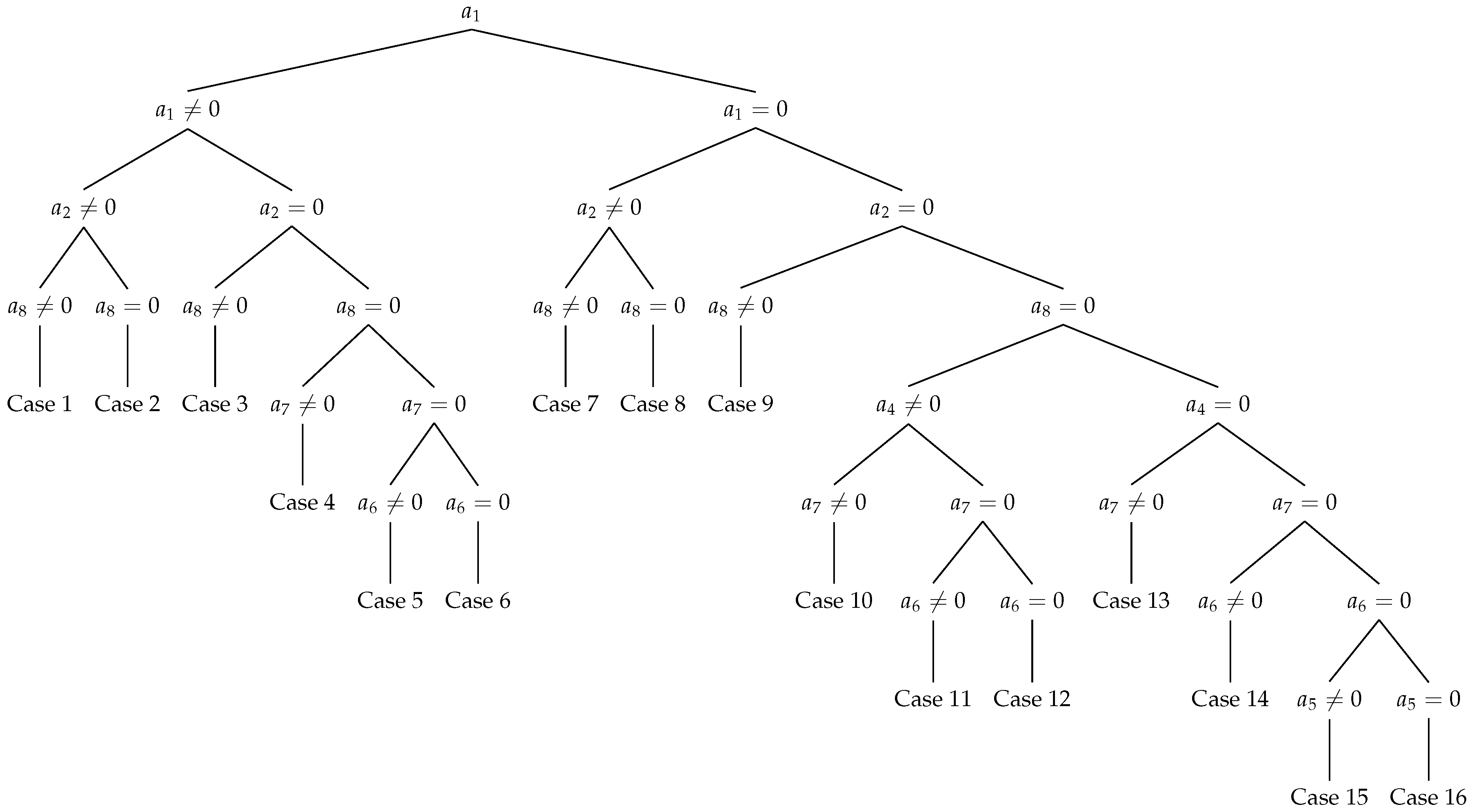 

Let X and $\tilde{X}$ be two elements in the Lie algebra ${\mathcal{L}}^8$ with basis (9) given by $X={\sum }_{i=1}^8{a}_i{X}_i$ and $\tilde{X}={\sum }_{i=1}^8{\tilde{a}}_i{X}_i$. For simplicity, we will write X and $\tilde{X}$ as row vectors of the coefficients on the form $X=(a_1{a}_2...a_8)$ and $\tilde{X}=(\widetilde{a_1}\widetilde{a_2}...\widetilde{a_8})$. Then, in order that X and $\tilde{X}$ are in the same conjugacy class, we must have $\tilde{X}=XA$, where A is given by (15). Therefore, the theorem is proven by solving the system:

$$\begin{array}{c}\widetilde{a_1}=a_1,\hfill \\ \widetilde{a_2}=a_2,\hfill \\ \widetilde{a_3}=a_1{ϵ}_4+\frac{EI}{k}{a}_2{ϵ}_7-a_2{ϵ}_5+a_3-a_4{ϵ}_1+a_5{ϵ}_2-\frac{1}{2}{a}_6{ϵ}_2^2+\frac{1}{6}{a}_7{ϵ}_2^3-\frac{EI}{k}{a}_7{ϵ}_2-\frac{1}{24}{a}_8{ϵ}_2^4+\frac{1}{2}\frac{EI}{{\rho }_1}{a}_8{ϵ}_1^2+\frac{1}{2}\frac{EI}{k}{a}_8{ϵ}_2^2,\hfill \\ \widetilde{a_4}=\frac{EI}{{\rho }_1}{a}_1{ϵ}_8-\frac{EI}{{\rho }_1}{a}_8{ϵ}_1+a_4,\hfill \\ \widetilde{a_5}=a_2{ϵ}_6+a_5-a_6{ϵ}_2+\frac{1}{2}{a}_7{ϵ}_2^2-\frac{1}{6}{a}_8{ϵ}_2^3,\hfill \\ \widetilde{a_6}=a_2{ϵ}_7+a_6-a_7{ϵ}_2+\frac{1}{2}{a}_8{ϵ}_2^2,\hfill \\ \widetilde{a_7}=a_2{ϵ}_8-a_8{ϵ}_2+a_7,\hfill \\ \widetilde{a_8}=a_8,\hfill \end{array}$$

(17)

for ${\left\{{ϵ}_i\right\}}_{i=1}^8$ in terms of ${\left\{a_i\right\}}_{i=1}^8$ in order to get the simplest values of ${\left\{{\tilde{a}}_i\right\}}_{i=1}^8$.

The results are presented for different cases in a tree diagram, where each of its vertices is an invariant function, and its leaves are given completely. Moreover, one can verify that all of the parameters $\alpha ,\beta$ and γ appearing in each case are invariants. Therefore, the inequivalence and completeness conditions are satisfied.

All joint invariants are obtained by solving the following system of PDEs, which is given by using Formula (2):

$$\begin{array}{c}\left\{\begin{array}{c}{a}_4\frac{\partial \Phi }{\partial a_3}+\frac{EI}{{\rho }_1}{a}_8\frac{\partial \Phi }{\partial a_4}=0,\hfill \\ a_5\frac{\partial \Phi }{\partial a_3}-\frac{EI}{k}{a}_7\frac{\partial \Phi }{\partial a_3}-a_6\frac{\partial \Phi }{\partial a_5}-a_7\frac{\partial \Phi }{\partial a_6}-a_8\frac{\partial \Phi }{\partial a_7}=0,\hfill \\ a_1\frac{\partial \Phi }{\partial a_3}=0,\hfill \\ a_2\frac{\partial \Phi }{\partial a_3}=0,\hfill \\ a_2\frac{\partial \Phi }{\partial a_5}=0,\hfill \\ a_2\frac{\partial \Phi }{\partial a_6}+\frac{EI}{k}{a}_2\frac{\partial \Phi }{\partial a_3}=0,\hfill \\ a_2\frac{\partial \Phi }{\partial a_7}+\frac{EI}{{\rho }_1}{a}_1\frac{\partial \Phi }{\partial a_4}=0.\hfill \end{array}\right.\hfill \end{array}$$

(18)

By solving this system, we obtain $\Phi (a_1,a_2,a_3,a_4,a_5,a_6,a_7,a_8)=F(a_1,a_2,a_8)$, where Fis an arbitrary function of $a_1,a_2,a_8$. Hence, the basic invariants of Timoshenko System (1) are $a_1,a_2$ and $a_8$; this means that the first three vertices of the tree will be these invariants in any order. In our case, we will consider the order $a_1,a_2,a_8$.

The full details for each leaf are given as follows:

Case 1

$a_1\ne 0$, $a_2\ne 0$, $a_8\ne 0$: Let ${ϵ}_2={ϵ}_3={ϵ}_5=0$, ${ϵ}_1=\frac{{\rho }_1{a}_2{a}_4-EI{a}_7}{EI{a}_2{a}_8}$, ${ϵ}_4=\frac{{\rho }_1}{EI}\frac{a_4^2}{a_8}+\frac{EI}{k}{a}_6-a_3-\frac{EI}{2{\rho }_1}\frac{a_7^2}{a_2^2{a}_8}$, ${ϵ}_6=-\frac{a_5}{a_2}$, ${ϵ}_7=-\frac{a_6}{a_2}$ and ${ϵ}_8=-\frac{a_7}{a_2}$ to have $\widetilde{a_3}=\widetilde{a_4}=\widetilde{a_5}=\widetilde{a_6}=\widetilde{a_7}=0$: the conjugacy class is $⟨X_1+\alpha X_2+\beta X_8⟩$, with $\alpha ,\beta \ne 0$.

Case 2

$a_1\ne 0$, $a_2\ne 0$, $a_8=0$: Let ${ϵ}_1={ϵ}_2={ϵ}_3={ϵ}_5=0$, ${ϵ}_4=\frac{EI}{k}{a}_6-a_3$, ${ϵ}_6=-\frac{a_5}{a_2}$, ${ϵ}_7=-\frac{a_6}{a_2}$, ${ϵ}_8=-\frac{a_7}{a_2}$ to have $\widetilde{a_3}=\widetilde{a_5}=\widetilde{a_6}=\widetilde{a_7}=0$. The conjugacy class is $⟨X_1+\alpha X_2+\beta X_4⟩$, with $\alpha \ne 0$, $\beta \in \mathbb{R}$.

Case 3

$a_1\ne 0$, $a_2=0$, $a_8\ne 0$: Let ${ϵ}_1=0$, ${ϵ}_2=\frac{a_7}{a_8}$, ${ϵ}_4=\frac{EI}{2k}\frac{a_7^2}{a_8}-a_3-\frac{a_5{a}_7}{a_8}+\frac{a_6{a}_7^2}{2a_8^2}-\frac{a_7^4}{8a_8^3}$ and ${ϵ}_8=-\frac{{\rho }_1}{EI}{a}_4$ to make $\widetilde{a_3}=\widetilde{a_4}=\widetilde{a_7}=0$: the conjugacy class is $⟨X_1+\alpha X_5+\beta X_6+\gamma X_8⟩$, $\alpha ,\beta \in \mathbb{R}$, $\gamma \ne 0$.

When $a_1\ne 0$, $a_2=0$, $a_8=0$, we need to solve system (18) again to see what are the invariants as well the next vertices of the tree.

Solving system (18) taking into account that $a_2=a_8=0$ gives $\Phi (a_1,a_2,a_3,a_4,a_5,a_6,a_7,a_8)=F(a_1,a_7,-2a_5{a}_7+a_6^2)$, so we can consider $a_7$ to be the next vertex of the tree.

Case 4

$a_1\ne 0$, $a_2=0$, $a_8=0$, $a_7\ne 0$: Let ${ϵ}_1=0$, ${ϵ}_2=\frac{a_6}{a_7}$, ${ϵ}_4=\frac{EI}{k}{a}_6-a_3-\frac{a_5{a}_6}{a_7}+\frac{a_6^2}{3a_7^2}$ and ${ϵ}_8=-\frac{{\rho }_1}{EI}{a}_4$ to make $\widetilde{a_3}=\widetilde{a_4}=\widetilde{a_6}=\widetilde{a_8}=0$: the conjugacy class is of the form $⟨X_1+\alpha X_5+\beta X_7⟩$, $\alpha \in \mathbb{R},\beta \ne 0$.

Again, for the case $a_1\ne 0$, $a_2=0$, $a_8=0$, $a_7=0$, we resolve system (18) to have $\Phi (a_1,a_2,a_3,a_4,a_5,a_6,a_7,a_8)=F(a_1,a_6)$, so next vertex can be $a_6$:

Case 5

$a_1\ne 0$, $a_2=0$, $a_8=0$, $a_7=0$, $a_6\ne 0$: Let ${ϵ}_1=0$, ${ϵ}_2=\frac{a_5}{a_6}$, ${ϵ}_4=-a_3-\frac{a_5^2}{2a_6}$ and ${ϵ}_8=-\frac{{\rho }_1}{EI}{a}_4$ to make $\widetilde{a_3}=\widetilde{a_4}=\widetilde{a_5}=0$: the corresponding conjugacy class is $⟨X_1+\alpha X_6⟩$, where $\alpha \ne 0$.

Case 6

$a_1\ne 0$, $a_2=0$, $a_8=0$, $a_7=0$, $a_6=0$: Let ${ϵ}_1={ϵ}_2=0$, ${ϵ}_4=-a_3$ and ${ϵ}_8=-\frac{{\rho }_1}{EI}{a}_4$ to make $\widetilde{a_3}=\widetilde{a_4}=0$: the conjugacy class is $⟨X_1+\alpha X_5⟩$, $\alpha \in \mathbb{R}$.

Case 7

$a_1=0$, $a_2\ne 0$, $a_8\ne 0$: Let ${ϵ}_1=\frac{{\rho }_1}{EI}\frac{a_4}{a_8}$, ${ϵ}_2=0$, ${ϵ}_5=a_3-\frac{EI}{k}{a}_6-\frac{{\rho }_1}{2EI}\frac{a_4^2}{a_8}$, ${ϵ}_6=-a_5$, ${ϵ}_7=-a_6$ and ${ϵ}_8=-a_7$ to make $\widetilde{a_3}=\widetilde{a_4}=\widetilde{a_5}=\widetilde{a_6}=\widetilde{a_7}=0$: the conjugacy class is $⟨X_2+\alpha X_8⟩$, $\alpha \ne 0$.

Case 8

$a_1=0$, $a_2\ne 0$, $a_8=0$: Let ${ϵ}_2=0$, ${ϵ}_5=a_3-{ϵ}_1{a}_4-\frac{EI}{k}{a}_6$, ${ϵ}_6=-a_5$, ${ϵ}_7=-a_6$ and ${ϵ}_8=-a_7$ to make $\widetilde{a_3}=\widetilde{a_5}=\widetilde{a_6}=\widetilde{a_6}=\widetilde{a_7}=0$: the conjugacy class is $⟨X_2+\alpha X_4⟩$, $\alpha \in \mathbb{R}$.

Case 9

$a_1=0$, $a_2=0$, $a_8\ne 0$: Let ${ϵ}_1=\frac{{\rho }_1}{EI}{a}_4$ and ${ϵ}_2=a_7$, to get $\widetilde{a_4}=\widetilde{a_7}=0$: the conjugacy class is of the form $⟨\alpha X_3+\beta X_5+\gamma X_6+X_8⟩$, $\alpha ,\beta ,\gamma \in \mathbb{R}$.

By substituting $a_1=a_2=a_8=0$ in system (18) and solving it, we get $\Phi (a_1,a_2,a_3,a_4,a_5,a_6,a_7,a_8)=F(a_4,a_7,-2a_5{a}_7+a_6^2)$. So the next two vertices can be $a_4$ and $a_7$ in any order. We consider the order $a_4$, $a_7$.

Case 10

$a_1=0$, $a_2=0$, $a_8=0$, $a_4\ne 0$, $a_7\ne 0$: Let ${ϵ}_1=-\frac{EI}{k}{a}_6+a_3+\frac{a_5{a}_6}{a_7}-\frac{a_6^3}{3a_7^2}$ and ${ϵ}_2=\frac{a_6}{a_7}$ to make $\widetilde{a_3}=\widetilde{a_6}=0$: the conjugacy class is $⟨X_4+\alpha X_5+\beta X_7⟩$, $\alpha \in \mathbb{R},\beta \ne 0$.

In case $a_1=a_2=a_8=a_7=0$, solving system (18) yields $\Phi (a_1,a_2,a_3,a_4,a_5,a_6,a_7,a_8)=F(a_4,a_6)$ which implies, after considering $a_4$ and $a_7$ as vertices, that one can consider the invariant $a_6$ as a new vertex.

Case 11

$a_1=0$, $a_2=0$, $a_8=0$, $a_4\ne 0$, $a_7=0$, $a_6\ne 0$: Let ${ϵ}_1=\frac{a_5^2}{2a_6}+a_3$ and ${ϵ}_2=\frac{a_5}{a_6}$ to make $\widetilde{a_3}=\widetilde{a_5}=0$: the conjugacy class is $⟨X_4+\alpha X_6⟩$, with $\alpha \ne 0$.

Case 12

$a_1=0$, $a_2=0$, $a_8=0$, $a_4\ne 0$, $a_7=0$, $a_6=0$: Let ${ϵ}_1=a_3$, ${ϵ}_2=0$ to make $\widetilde{a_3}=0$: then the conjugacy class is $⟨X_4+\alpha X_5⟩$, $\alpha \in \mathbb{R}$.

Case 13

$a_1=0$, $a_2=0$, $a_8=0$, $a_4=0$, $a_7\ne 0$: Let ${ϵ}_2=a_6$ to have $\widetilde{a_6}=0$: the conjugacy class is $⟨\alpha X_3+\beta X_5+X_7⟩$, $\alpha ,\beta \in \mathbb{R}$.

Case 14

$a_1=0$, $a_2=0$, $a_8=0$, $a_4=0$, $a_7=0$, $a_6\ne 0$: Let ${ϵ}_2=a_5$ to have $\widetilde{a_5}=0$: the conjugacy class is $⟨\alpha X_3+X_6⟩$, $\alpha \in \mathbb{R}$.

When $a_6=0$ with $a_1=a_2=a_8=a_4=a_7=0$, solving the PDEs system (18) gives $\Phi (a_1,a_2,a_3,a_4,a_5,a_6,a_7,a_8)=F(a_5)$. So the next invariant vertex is $a_5$.

Case 15

$a_1=0$, $a_2=0$, $a_8=0$, $a_4=0$, $a_7=0$, $a_6=0$, $a_5\ne 0$: Let ${ϵ}_2=-a_3$ to have $\widetilde{a_3}=0$: the conjugacy class is $⟨X_5⟩$.

Case 16

$a_1=0$, $a_2=0$, $a_8=0$, $a_4=0$, $a_7=0$, $a_6=0$, $a_5=0$: the conjugacy class is $⟨X_3⟩$. ☐

5. Optimal Reductions and Invariant Solutions

It is known that the invariant solutions for PDEs can be determined by two procedures, namely the invariant form method and the direct substitution method [14]. The idea of looking for group invariant solutions generalizes quite naturally to PDEs with any number of independent and dependent variables. A one parameter group that acts nontrivially on one or more independent variables can be used to reduce the number of independent variables by one.

In this section, we focus on the invariant form method, which requires that at least one of the infinitesimals ${\xi }^1$ and ${\xi }^2$ is not equal to zero [9,14]. Basically, the reason is that a vector field of the type $X={\eta }_1\frac{\partial }{\partial \phi }+{\eta }_2\frac{\partial }{\partial \psi }$ cannot leave the submanifold of codimension two defined by the equations $\phi =f(t,x)$ and $\psi =g(t,x)$ invariant, otherwise the dimension of the solution space would go down. This means the transversality condition in the sense of [16] will not be satisfied. For this reason, only the generators $X^1,\dots ,X^8$ from system (16) are considered in this section.

We solve the invariance surface conditions explicitly by solving the corresponding characteristic equation given by:

$$\frac{dt}{{\xi }^1(t,x,\phi ,\psi )}=\frac{dx}{{\xi }^2(t,x,\phi ,\psi )}=\frac{d\phi }{{\eta }^1(t,x,\phi ,\psi )}=\frac{d\psi }{{\eta }^2(t,x,\phi ,\psi )},$$

(19)

to get the corresponding invariants, which are used to reduce the number of independent variables by one. The procedure is explained in detail in the following example. Moreover, all possible invariant variables of the optimal system (16) and their corresponding reductions are given in Table 2.

Table 2. Reductions using one-dimensional optimal System (16).

Generators in (16)	Invariant Variables	The Reduced System
$X^1=X_1+\alpha X_2+\beta X_8,$	A	$(k-{\alpha }^2{\rho }_1)Z^{″}+k{W}^{\prime }+\frac{\alpha \beta {\rho }_{1}EI}{k}\zeta +\frac{1}{6}\left(\frac{\beta k}{\alpha }-\alpha \beta {\rho }_1\right){\zeta }^3=0,$
$\alpha ,\beta \ne 0.$		$({\rho }_2{\alpha }^2-EI)W^{″}+k{Z}^{\prime }+kW+\chi \left(-\alpha W^{\prime }\right)-\frac{\beta EI}{2\alpha }{\zeta }^2+\frac{\beta k}{24\alpha }{\zeta }^4=0.$
$X^2=X_1+\alpha X_2+\beta X_4,$	B	$(k-{\alpha }^2{\rho }_1)Z^{″}+k{W}^{\prime }-\beta {\rho }_1=0,$
$\alpha \ne 0,\beta \in \mathbb{R}.$		$({\rho }_2{\alpha }^2-EI)W^{″}-k{Z}^{\prime }+kW+\chi \left(-\alpha W^{\prime }\right)=0.$
$X^3=X_1+\alpha X_5+\beta X_6+\gamma X_8,$	C	$Z^{″}+W^{\prime }=0,$
$\alpha ,\beta \in \mathbb{R},\gamma \ne 0.$		$EI{W}^{″}-k{Z}^{\prime }-kW-\chi \left(\frac{\gamma }{6}{\zeta }^3+\beta \zeta +\alpha \right)=0.$
$X^4=X_1+\alpha X_5+\beta X_7,$	D	$Z^{″}+W^{\prime }=0,$
$\alpha \in \mathbb{R},\beta \ne 0.$		$EI{W}^{″}-k{Z}^{\prime }-kW-\chi \left(\alpha +\frac{\beta }{2}{\zeta }^2\right)=0.$
$X^5=X_1+\alpha X_6,$	E	$Z^{″}+W^{\prime }=0,$
$\alpha \ne 0.$		$EI{W}^{″}-k{Z}^{\prime }-kW-\chi \left(\alpha \zeta \right)=0.$
$X^6=X_1+\alpha X_5,$	F	$Z^{″}+W^{\prime }=0,$
$\alpha \in \mathbb{R}.$		$EI{W}^{″}-k{Z}^{\prime }-kW-\chi \left(\alpha \right)=0.$
$X^7=X_2+\alpha X_8,$	G	${\rho }_1{Z}^{″}=0,$
$\alpha \ne 0.$		${\rho }_2{W}^{″}+\chi \left(W^{\prime }\right)+kW+\frac{\alpha EIk}{2{\rho }_1}{\zeta }^2=0.$
$X^8=X_2+\alpha X_4,$	H	${\rho }_1{Z}^{″}=0,$
$\alpha \in \mathbb{R}.$		${\rho }_2{W}^{″}+\chi \left(W^{\prime }\right)+kW+\alpha k\zeta =0.$

As another application for the optimal system based on the definition of the invariant boundary value problem given in [14,17], we classify the non-similar invariant conditions prescribed on invariant surfaces under symmetry transformations for Timoshenko system (1) as given in Table 3. This is achieved by finding invariant conditions as arbitrary functions of the invariants up to the first order and invariant surfaces as arbitrary functions of the invariants of order zero, which depend on the independent variables for each generator in the optimal system (16).

Table 3. Invariant conditions prescribed on invariant surfaces and theirs reductions.

${\mathit{X}}^{\mathit{i}}$	Invariant Condition	Invariant Surface	Reduced Invariant Condition	Reduced Invariant Surface
$X^1$	$\widehat{A}$	$\omega (x-\alpha t)$	$B\left(\zeta ,Z,W,\frac{\beta EI}{2k}{\zeta }^2-\frac{\beta }{24}{\zeta }^4-\alpha Z^{\prime },Z^{\prime },-\alpha W^{\prime },W^{\prime }\right)$	$\omega (\zeta )$
$X^2$	$\widehat{B}$	$\omega (x-\alpha t)$	$B\left(\zeta ,Z,W,\alpha Z^{\prime },Z^{\prime },\alpha W^{\prime },W^{\prime }\right)$	$\omega (\zeta )$
$X^3$	$\widehat{C}$	$\omega (x)$	$B\left(\zeta ,Z,W,-\alpha \zeta -\left(\frac{\beta }{2}+\frac{\gamma EI}{2k}\right){\zeta }^2-\frac{\gamma }{24}{\zeta }^4,Z^{\prime },\alpha +\beta \zeta +\frac{\gamma }{6}{\zeta }^3,W^{\prime }\right)$	$\omega (\zeta )$
$X^4$	$\widehat{D}$	$\omega (x)$	$B\left(\zeta ,Z,W,\left(\frac{EI}{k}\beta -\alpha \right)\zeta -\frac{\beta }{6}{\zeta }^3,Z^{\prime },\alpha +\frac{\beta }{2}{\zeta }^2,W^{\prime }\right)$	$\omega (\zeta )$
$X^5$	$\widehat{E}$	$\omega (x)$	$B\left(\zeta ,Z,W,-\frac{\alpha }{2}{\zeta }^2,Z^{\prime },\alpha \zeta ,W^{\prime }\right)$	$\omega (\zeta )$
$X^6$	$\widehat{F}$	$\omega (x)$	$B(\zeta ,Z,W,-\alpha \zeta ,Z^{\prime },\alpha ,W^{\prime })$	$\omega (\zeta )$
$X^7$	$\widehat{G}$	$\omega \left(t\right)$	$B\left(\zeta ,Z,W,Z^{\prime },\frac{\alpha EI}{2{\rho }_1}{\zeta }^2,W^{\prime },0\right)$	$\omega (\zeta )$
$X^8$	$\widehat{H}$	$\omega \left(t\right)$	$B\left(\zeta ,Z,W,Z^{\prime },\alpha \zeta ,W^{\prime },0\right)$	$\omega (\zeta )$

Example 1.

Reduction and invariant solution using $X^6$:

Consider the generator $X^6=X_1+\alpha X_5=\frac{\partial }{\partial t}-\alpha x\frac{\partial }{\partial \phi }+\alpha \frac{\partial }{\partial \psi }$ where $\alpha \in \mathbb{R}$, from the optimal system (16). Solving the corresponding characteristic equations of the first prolongation:

$$\frac{dt}{1}=\frac{dx}{0}=\frac{d\phi }{-\alpha x}=\frac{d\psi }{\alpha }=\frac{d{\phi }_t}{0}=\frac{d{\phi }_x}{-\alpha }=\frac{d{\psi }_t}{0}=\frac{d{\psi }_x}{0},$$

gives the following invariants up to the first order:

$$\begin{array}{ccccccc}{I}_1=x,& I_2=\phi +\alpha tx,& I_3=\psi -\alpha t,& I_4={\phi }_t,& I_5={\phi }_x+\alpha t,& I_6={\psi }_t,& I_7={\psi }_x.\end{array}$$

(20)

Since the order of the Timoshenko system (1) is two, then the invariant conditions have to be functions of the first order invariants of the form:

$$B_{\Gamma }(I_1,I_2,I_3,I_4,I_5,I_6,I_7)=0,\Gamma =1,\dots ,4.$$

(21)

The invariant conditions (21) are prescribed on the invariant surfaces:

$${\omega }_{\gamma }(I_1)=0,\gamma =1,2,$$

(22)

which are invariants of order zero that depend on the independent variables.

For $\alpha \ne 0$, if we restrict the invariant conditions (21) to be linear, then it will take the form:

$$\begin{array}{cc}{B}_{\Gamma }=\hfill & A_{\Gamma ,1}(x)+A_{\Gamma ,2}(x)(\phi +\alpha tx)+A_{\Gamma ,3}(x)(\psi -\alpha t)+A_{\Gamma ,4}(x){\phi }_t+A_{\Gamma ,5}(x)({\phi }_x+\alpha t)\hfill \\ & +A_{\Gamma ,6}(x){\psi }_t+A_{\Gamma ,7}(x){\psi }_x=0,\hfill \end{array}$$

(23)

where $A_{\Gamma ,i}(x)$ are arbitrary functions for $\Gamma =1,\dots ,4$ and $i=1,\dots ,7$.

Moreover, the invariants of order zero $I_1,I_2$ and $I_3$ give the invariant variables:

$$\begin{array}{ccc}\phi (t,x)=Z(\zeta )-\alpha tx,& \psi (t,x)=W(\zeta )+\alpha t,& \zeta =x.\end{array}$$

(24)

The reduction of Timoshenko System (1) with the boundary conditions (23) prescribed on the surfaces $x=0$ and $x=L$ using the invariant variables (24 is the system of ODEs of the form:

$$\begin{array}{c}{Z}^{″}+W^{\prime }=0,\hfill \\ EI{W}^{″}-k{Z}^{\prime }-kW-\chi \left(\alpha \right)=0,\hfill \end{array}$$

(25)

with general boundary conditions of the form:

$$\begin{array}{c}{A}_{\Gamma ,1}(\zeta )+A_{\Gamma ,2}(\zeta )Z+A_{\Gamma ,3}(\zeta )W-\alpha A_{\Gamma ,4}(\zeta )\zeta +A_{\Gamma ,5}(\zeta )Z^{\prime }+\alpha A_{\Gamma ,6}(\zeta )+A_{\Gamma ,7}(\zeta )W^{\prime }=0\hfill \end{array}$$

(26)

prescribed on the surfaces $\zeta =0$ and $\zeta =L$.

For instance, we consider a beam that models small motions of a hinged arm, which is hinged at the origin and free at its other end. This case was considered in [18] with two control functions. The control functions are the force $f(t)$ applied at the free end and a torque $\tau (t)$ applied at the hinged end. The associated boundary conditions:

$$\begin{array}{cccc}\phi (t,0)=0,& {\psi }_x(t,0)=\tau (t),& {\phi }_x(t,L)-\psi (t,L)=f(t),& {\psi }_x(t,L)=0,\end{array}$$

(27)

can be obtained from Equation (23) for the non-zero values $A_{1,2}=1$ at $x=0$; $A_{2,1}=-r$, $A_{2,7}=1$ at $x=0$; $A_{3,1}=-q$, $A_{3,3}=-1$, $A_{3,5}=1$ at $x=L$; $A_{4,7}=1$ at $x=L$ with force $f(t)=q-2\alpha t$ and torque $\tau (t)=r$.

Using the invariant variables (24), the boundary conditions (27) are reduced to:

$$\begin{array}{cccc}Z(0)=0,& W^{\prime }(0)=r,& Z^{\prime }(L)-W(L)=q,& W^{\prime }(L)=0.\end{array}$$

(28)

The solution of the boundary value problem (25) and (28) is given by:

$$\begin{array}{c}Z\left(\zeta \right)=\frac{r}{6L}{\zeta }^3-\frac{r}{2}{\zeta }^2+\left(\frac{Lr}{2}-\frac{rEI}{2Lk}-\frac{\chi \left(\alpha \right)}{2k}+\frac{q}{2}\right)\zeta ,\hfill \\ W\left(\zeta \right)=-\frac{r}{2L}{\zeta }^2+r\zeta -\frac{\chi \left(\alpha \right)}{2k}-\frac{1}{2}\left(q+r\left(\frac{EI}{Lk}+L\right)\right).\hfill \end{array}$$

(29)

Substituting back in the invariant variables (24), the system (1) with the boundary conditions (27) has the following solution:

$$\begin{array}{c}\phi \left(t,x\right)=\frac{r}{6L}{x}^3-\frac{r}{2}{x}^2+\left(-\alpha t-\frac{\chi \left(\alpha \right)}{2k}-\frac{rEI}{2Lk}+\frac{q}{2}+\frac{rL}{2}\right)x,\hfill \\ \psi \left(t,x\right)=\alpha t-\frac{r}{2L}{x}^2+rx-\frac{\chi \left(\alpha \right)}{2k}-\frac{1}{2}\left(q+r\left(\frac{EI}{Lk}+L\right)\right).\hfill \end{array}$$

(30)

$$\begin{array}{cc}A:\hfill & \phi (t,x)=Z(\zeta )-\frac{\beta }{24}t{x}^4+\frac{\beta EI}{2k}t{x}^2+\frac{\alpha \beta }{12}{t}^2{x}^3-\frac{\alpha \beta EI}{2k}{t}^{2}x+\frac{\beta EI}{6{\rho }_1}{t}^3-\frac{{\alpha }^2\beta }{12}{x}^2{t}^3+\frac{{\alpha }^2\beta EI}{6k}{t}^3\hfill \\ & +\frac{{\alpha }^3\beta }{24}x{t}^4-\frac{{\alpha }^4}{120}{t}^5,\psi (t,x)=W(\zeta )+\frac{\beta }{24\alpha }{x}^4,\zeta =x-\alpha t.\hfill \\ B:\hfill & \phi (t,x)=Z(\zeta )+\frac{\beta }{2}{t}^2,\psi (t,x)=W(\zeta ),\zeta (t,x)=x-\alpha t.\hfill \\ C:\hfill & \phi (t,x)=Z(\zeta )-\alpha tx-\frac{\beta }{2}t{x}^2-\frac{\gamma }{24}t{x}^4+\frac{\gamma EI}{2k}t{x}^2+\frac{\gamma EI}{6{\rho }_1}{t}^3,\psi (t,x)=W(\zeta )+\alpha t\hfill \\ & +\beta tx+\frac{\gamma }{6}t{x}^3,\zeta =x.\hfill \\ D:\hfill & \phi (t,x)=Z(\zeta )+\left(\frac{\beta EI}{k}-\alpha \right)tx-\frac{\beta }{6}t{x}^3,\psi (t,x)=W(\zeta )+\alpha t+\frac{\beta }{2}t{x}^2,\zeta =x.\hfill \\ E:\hfill & \phi (t,x)=Z(\zeta )-\frac{\alpha }{2}{x}^{2}t,\psi (t,x)=W(\zeta )+\alpha xt,\zeta =x.\hfill \\ F:\hfill & \phi (t,x)=Z(\zeta )-\alpha tx,\psi (t,x)=W(\zeta )+\alpha t,\zeta =x.\hfill \\ G:\hfill & \phi (t,x)=Z(\zeta )+\frac{\alpha EI}{2{\rho }_1}{t}^{2}x+\frac{\alpha EI}{6k}{x}^3,\psi (t,x)=W(\zeta )+\frac{1}{24}\alpha x^4-\frac{\alpha }{120}{x}^5,\zeta =t.\hfill \\ H:\hfill & \phi (t,x)=Z(\zeta )+\alpha tx,\psi (t,x)=W(\zeta ),\zeta =t.\hfill \end{array}$$

(31)

$$\begin{array}{c}\hfill \begin{array}{cc}\widehat{A}:\hfill & B\left(x-\alpha t,\phi +\frac{{\alpha }^4\beta }{120}{t}^5-\frac{{\alpha }^3\beta }{24}{t}^{4}x-\frac{{\alpha }^2\beta EI}{6k}{t}^3+\frac{{\alpha }^2\beta }{12}{t}^3{x}^2-\frac{\beta EI}{6{\rho }_1}{t}^3-\frac{\alpha \beta }{12}{t}^2{x}^3+\frac{\alpha \beta EI}{2k}{t}^{2}x+\frac{\beta }{24}t{x}^4-\frac{\beta EI}{2k}t{x}^2\right.\hfill \\ & \left.,\psi -\frac{\beta }{24\alpha }{x}^4,{\phi }_t-\frac{\beta EI}{2{\rho }_1}{t}^2,{\phi }_x-\frac{\beta {\alpha }^3}{24}{t}^4+\frac{\beta {\alpha }^2}{6}{t}^{3}x+\frac{\alpha \beta EI}{2k}{t}^2-\frac{\alpha \beta }{4}{t}^2{x}^2+\frac{\beta }{6}t{x}^3-\frac{\beta EI}{k}tx,{\psi }_t,{\psi }_x-\frac{\beta }{6\alpha }{x}^3\right).\hfill \\ \widehat{B}:\hfill & B\left(x-\alpha t,\phi -\frac{\beta }{2}{t}^2,\psi ,{\phi }_t-\beta t,{\phi }_x,{\psi }_t,{\psi }_x\right).\hfill \\ \widehat{C}:\hfill & B\left(x,\phi +\alpha tx+\frac{\beta }{2}t{x}^2+\frac{\gamma }{24}t{x}^4-\frac{\gamma EI}{2k}t{x}^2-\frac{\gamma EI}{6{\rho }_1}{t}^3,\psi -\alpha t-\beta tx-\frac{\gamma }{6}t{x}^3,{\phi }_t-\frac{\gamma EI}{2{\rho }_1}{t}^2,{\phi }_x+\alpha t+\beta tx+\frac{\gamma }{6}t{x}^3\right.\hfill \\ & \left.-\frac{\gamma EI}{k}tx,{\psi }_t,{\psi }_x-\beta t-\frac{\gamma }{2}t{x}^2\right).\hfill \\ \widehat{D}:\hfill & B\left(x,\phi +\alpha tx+\frac{\beta }{6}t{x}^3-\frac{\beta EI}{k}tx,\psi -\alpha t-\frac{\beta }{2}t{x}^2,{\phi }_t,{\phi }_x+\alpha t+\frac{\beta }{2}t{x}^2-\frac{\beta EI}{k}t,{\psi }_t,{\psi }_x-\beta tx\right).\hfill \\ \widehat{E}:\hfill & B\left(x,\phi +\frac{\alpha }{2}t{x}^2,\psi -\alpha tx,{\phi }_t,{\phi }_x+\alpha tx,{\psi }_t,{\psi }_x-\alpha t\right).\hfill \\ \widehat{F}:\hfill & B\left(x,\phi +\alpha tx,\psi -\alpha t,{\phi }_t,{\phi }_x+\alpha t,{\psi }_t,{\psi }_x\right).\hfill \\ \widehat{G}:\hfill & B\left(t,\phi +\frac{\alpha }{120}{x}^5-\frac{\alpha EI}{6k}{x}^3-\frac{\alpha EI}{2{\rho }_1}{t}^{2}x,\psi -\frac{\alpha }{24}{x}^4,{\phi }_t-\frac{\alpha EI}{{\rho }_1}tx,{\phi }_x+\frac{\alpha }{24}{x}^4-\frac{\alpha EI}{2k}{x}^2,{\psi }_t,{\psi }_x-\frac{\alpha }{6}{x}^3\right).\hfill \\ \widehat{H}:\hfill & B\left(t,\phi -\alpha tx,\psi ,{\phi }_t-\alpha x,{\phi }_x,{\psi }_t,{\psi }_x\right).\hfill \end{array}\end{array}$$

(32)

6. Discussion and Concluding Remarks

The Lie group study of a nonlinear Timoshenko system of PDEs with the frictional damping term in rotational angle is performed. Lie symmetry generators and their Lie group transformations for the Timoshenko system are presented. A systematic approach and a formula for computing invariants in the adjoint representation is illustrated. Furthermore, the one-dimensional optimal system is derived for the corresponding Lie algebra. All possible invariant variables and their corresponding reductions for each vector field in the optimal system are found. The reductions to system of ordinary differential equations (ODEs) are given in Table 2. They are described by optimal reductions where all non-similar invariant solutions under symmetry transformations can be given from the solution of the reduced system of ODEs. The hinged-free beam with two control functions, constant torque applied at the hinged end and linear force applied at the free end, has been considered as an example. Finally, all possible non-similar invariant conditions prescribed on invariant surfaces under symmetry transformations are given in Table 3.

References

- Timoshenko, S.P. On the correction for shear of the differential equation for transverse vibrations of prismatic bars. Edinb. Dubl. Phil. Mag. 1921, 41, 744–746. [Google Scholar]
- Timoshenko, S.P. On the transverse vibrations of bars of uniform cross-section. Edinb. Dubl. Phil. Mag. 1922, 43, 125–131. [Google Scholar]
- Chalishajar, D.; Lipscomb, B. On applications of generalized functions in the discontinuous beam bending differential equations. Appl. Math. 2016, 7, 1943. [Google Scholar]
- Mustafa, M.I.; Messaoudi, S.A. General energy decay rates for a weakly damped Timoshenko system. J. Dyn. Control Syst. 2010, 16, 211–226. [Google Scholar]
- Alabau-Boussouira, F. Strong lower energy estimates for nonlinearly damped Timoshenko beams and Petrowsky equations. NoDEA 2011, 18, 571–597. [Google Scholar]
- Ovsiannikov, L.V. Group analysis of differential equations; Academic Press: New York, NY, USA, 1982. [Google Scholar]
- Ibragimov, N.H. Selected works; ALGA Publ: Karlskrona, Sweden, 2006; Volume II. [Google Scholar]
- Olver, P.J. Applications of lie groups to differential equations; Springer Science and Business Media: Berlin, Germany, 2000; Volume 107. [Google Scholar]
- Hydon, P.E.; Hydon, E. Symmetry methods for differential equations: A beginner’s guide; Cambridge University Press: Cambridge, UK, 2000; Volume 22. [Google Scholar]
- Azad, H.; Biswas, I.; Ghanam, R.; Mustafa, M.T. On computing joint invariants of vector fields. J. Geom. Phys. 2015, 97, 69–76. [Google Scholar]
- Kotz, H. A Technique to classify the similarity solutions of nonlinear partial (integro-) differential equations. I. Optimal Systems of Solvable Lie Subalgebras. Z. Naturforsch. Phys. Sci. 1992, 47, 1161–1174. [Google Scholar]
- Hu, X.; Li, Y.; Chen, Y. A direct algorithm of one-dimensional optimal system for the group invariant solutions. J. Math. Phys. 2015, 56, 53504. [Google Scholar]
- Ibragimov, N.H. CRC Handbook of Lie Group Analysis of Differential Equations; CRC Press: Boca Raton, FL, USA, 1995; Volume 3. [Google Scholar]
- Bluman, G.; Anco, S.C. Symmetry and iNtegration Methods for Differential Equations; Springer Science and Business Media: Berlin, Germany, 2002; Volume 154. [Google Scholar]
- Blinkov, Y.A.; Carlos, F.C.; Vladimir, P.G.; Wilhelm, P.; Daniel, R. The MAPLE package Janet: II. linear partial differential equations. In Proceedings of the 6th International Workshop on Computer Algebra in Scientific Computing, Passau, Germany, 20–26 September 2003; pp. 41–54. [Google Scholar]
- Grundland, A.M.; Tempesta, P.; Winternitz, P. Weak transversality and partially invariant solutions. J. Math. Phys. 2003, 44, 2704–2722. [Google Scholar]
- Ibragimov, N.H. Selected Works; Alga Publications: Karlskrona, Sweden, 2001; Volume 1–2. [Google Scholar]
- Taylor, S.W. A smoothing property of a hyperbolic system and boundary controllability. J. Comput. Appl. Math. 2000, 1, 23–40. [Google Scholar]
© 2017 by the authors. Licensee MDPI, Basel, Switzerland. This article is an open access article distributed under the terms and conditions of the Creative Commons Attribution (CC BY) license (http://creativecommons.org/licenses/by/4.0/).