1. Introduction
In this paper, we are interested in the numerical solution of large scale nonsymmetric Stein matrix equations of the form:
where
A and
B are real, sparse and square matrices of size
and
respectively, and
E and
F are matrices of size
and
, respectively.
Stein matrix equations play an important role in many problems in control and filtering theory for discrete-time large-scale dynamical systems, in each step of Newton’s method for discrete-time algebraic Riccati equations, model reduction problems, image restoration techniques and other problems [
1,
2,
3,
4,
5,
6,
7,
8,
9,
10].
Direct methods for solving the matrix Equation (
1), such as those proposed by Bartels–Stewart [
11] and the Hessenberg–Schur [
12] algorithms, are attractive if the matrices are of small size. For a general overview of numerical methods for solving the Stein matrix equation [
1,
2,
13].
The Stein matrix Equation (
1) can be formulated as an
large linear system using the Kronecker formulation:
where
is the vector obtained by stacking all the columns of the matrix
X,
is the
n-by-
n identity matrix, and the Kronecker product of two matrices
A and
B is defined by
where
. This product satisfies the properties
,
and
. Then, the matrix Equation (
1) has a unique solution if and only if
for all
and
, where
denotes the spectrum of the matrix
A. Throughout the paper, we assume that this condition is satisfied. Moreover, if both
A and
B are Schur stable, i.e.,
and
lie in the open unit disc, and then the solution of Equation (
1) can be expressed as the following infinite matrix series:
To solve large linear matrix equations, several Krylov subspace projection methods have been proposed (see, e.g., [
1,
13,
14,
15,
16,
17,
18,
19,
20,
21,
22,
23,
24] and the references therein). The main idea developed in these methods is to use a block Krylov subspace or an extended block Krylov subspace and then project the original large matrix equation onto these Krylov subspaces using a Galerkin condition or a minimization property of the obtained residual. Hence, we will be interested in these two procedures to get approximate solutions to the solution of the Stein matrix Equation (
1). The rest of the paper is organized as follows. In the next section, we recall the extended block Krylov subspace and the extended block Arnoldi (EBA) algorithm with some properties. In
Section 3, we will apply the Galerkin approach (GA) to Stein matrix equations by using the extended Krylov subspaces. In
Section 4, we define the minimal residual (MR) method for Stein matrix equations by using the extended Krylov subspaces. We finally present some numerical experiments in
Section 5.
2. The Extended Block Krylov Subspace Algorithm
In this section, we recall the EBA algorithm applied to
where
. The block Krylov subspace associated with
is defined as:
The extended block Krylov subspace associated with the pair
is given as:
The EBA Algorithm 1 is defined as follows [
15,
16,
18,
23]:
| Algorithm 1. The Extended Block Arnoldi (EBA) Algorithm |
- (1)
Inputs: A an matrix, V an matrix and m an integer - (2)
Compute the QR decomposition of , i.e., - (3)
Set - (4)
for - (a)
Set : first r columns of ; : second r columns of - (b)
; - (c)
Orthogonalize w.r. to to get , i.e.
- ∗
for - ∗
- ∗
- ∗
End for
- (d)
Compute the decomposition of , i.e.,
- (5)
End For
|
This algorithm allows us to construct an orthonormal matrix that is a basis of the block extended Krylov subspace . The restriction of the matrix A to the block extended Krylov subspace is given by .
Let
. Then, we have the following relations [
25]:
where
is the matrix of the last
columns of the identity matrix
[
23,
25]. In the next section, we will define the GA for solving Stein matrix equations.
3. Galerkin-Based Methods
In this section, we will apply the Galerkin projection method to obtain low-rank approximate solutions of the nonsymmetric Stein matrix Equation (
1). This approach has been applied for Lyapunov, Sylvester or Riccati matrix equations [
1,
14,
15,
19,
20,
21,
23,
25,
26].
3.1. The Case: Both A and B Are Large Matrices
We consider here a nonsymmetric Stein matrix equation, where
A and
B are large and sparse matrices with
and
. We project the initial problem by using the extended block Krylov subspaces
and
associated with the pairs
and
, respectively, and get orthonormal bases
and
. We then consider approximate solutions of the Stein matrix Equation (
1) that have the low-rank form:
where
and
.
The matrix
is determined from the following Galerkin orthogonality condition:
Now, replacing
in Equation (
4), we obtain the reduced Stein matrix equation:
where
,
,
Assuming that
for any
and
, the solution
of the low-order Stein Equation (
5) can be obtained by a direct method such as those described in [
11]. The following result on the norm of the residual
allows us to stop the iterations without having to compute the approximation
.
Theorem 1. Let be the approximation obtained at step m by the EBA algorithm. Then, the Frobenius norm of the residual associated to the approximation is given by: where and: Proof. The proof is similar to the one given at proposition 6 in [
17]. ☐
In the following result, we give an upper bound for the norm of the error .
Theorem 2. Assume that and , and let be the exact solution of projected Stein matrix Equation (5) and be the approximate solution given by running m steps of the EBA algorithm. Then: Proof. The proof is similar to the one given at Theorem 2 in [
27]. ☐
The approximate solution
can be given as a product of two matrices of low rank. Consider the singular value decomposition of the
matrix:
where
is the diagonal matrix of the singular values of
sorted in decreasing order. Let
and
be the
matrices of the first
l columns of
and
respectively, corresponding to the
l singular values of magnitude greater than some tolerance. We obtain the truncated singular value decomposition:
where
. Setting
, and
it follows that:
This is very important for large problems when one doesn’t need to compute and store the approximation at each iteration.
The GA is given in Algorithm 2:
| Algorithm 2. Galerkin Approach (GA) for the Stein Matrix Equations |
- (1)
Inputs: A an matrix, B an matrix, E an matrix and F an matrix. - (2)
Choose a tolerance , a maximum number of iterations. - (3)
For - (4)
Compute , by Algorithm 1 applied to - (5)
Compute , by Algorithm 1 applied to - (6)
Solve the low order Stein Equation ( 5) and compute given by Equation ( 6) - (7)
if , stop, - (8)
Using Equation ( 8), the approximate solution is given by .
|
In the next section, we consider the case where the matrix A is large while B has a moderate or a small size.
3.2. The Case: A Large and B Small
In this section, we consider the Stein matrix equation:
where
E is a matrix of size
with
.
In this case, we will consider approximations of the exact solution
X as:
where
is the orthonormal basis obtained by applying the extended block Krylov subspace
. The orthogonality Galerkin condition gives:
where
is the
m-th residual given by
. Therefore, we obtain the projected Stein matrix equation:
where
and
.
The next result gives a useful expression of the norm of the residual.
Theorem 3. Let the exact solution of the reduced Stein matrix Equation (11) and let be the approximate solution of Equation (9) with the corresponding residual. Then: Proof. The residual is given by
. Since
E is belonging to
, then
. Using the relation
, we have:
As the matrix
is orthogonal and
, we have:
This result is very important because it allows us to calculate the Frobenius norm of without having to compute the approximate solution.
Next, we give a result showing that the error is an exact solution of a perturbed Stein matrix equation.
Theorem 4. Let be the approximate solution of Equation (9) obtained after m iterations of the EBA algorithm. Then:where Proof. Multiplying the Equation (
11) from the left by
, we obtain:
As
, we get:
where:
☐
We can now state the following result, which gives an upper bound for the norm of the error.
Theorem 5. If and , then we have: Proof. By subtracting Equation (
13) from Equation (
9), we get:
The error
is the solution of the Stein matrix Equation (
17) and can be expressed as:
☐
In the next section, we present projection methods based on extended block Krylov subspaces and MR property.
5. Numerical Experiments
In this section, we present some numerical experiments of large and sparse Stein matrix equations. We compared EBA-MR and EBA-GA methods. For the GA and at each iteration
m, we solved the projected Stein matrix equations by using the Bartels–Stewart algorithm [
11]. When solving the minimization reduced problem by the PGCG, we stopped the iterations when the relative norm of the residual was less than
or when a maximum of
iterations was achieved. The algorithms were coded in Matlab 8.0 (2014). The stopping criterion used for EBA-MR and GA was
or a maximum of
iterations was achieved.
In all of the examples, the coefficients of the matrices E and F were random values uniformly distributed on .
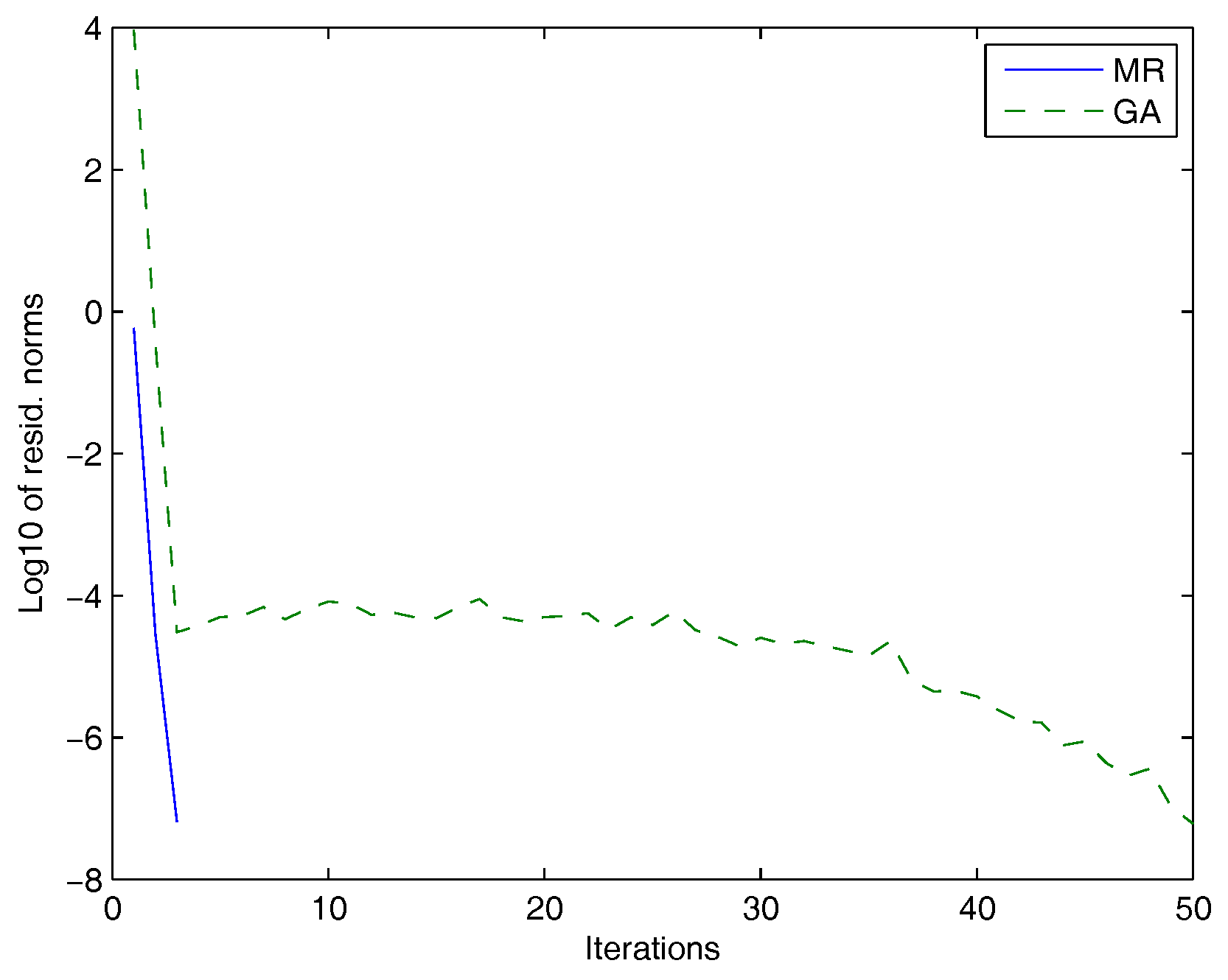
Example 1. In this first example, the matrices A and B are obtained from the centered finite difference discretization of the operators:on the unit square with homogeneous Dirichlet boundary conditions. The number of inner grid points in each direction was and for the operators and , respectively. The matrices A and B were obtained from the discretization of the operator and with the dimensions and , respectively. The discretization of the operator and yields matrices extracted from the Lyapack package [30] using the command fdm_2d_matrix and denoted as A = fdm(n0,’f_1(x,y)’,’f_2(x,y)’,’f(x,y)’). In this example, and , respectively, and are named as and with , , , , and . For this experiment, we used . In
Figure 1, we plotted the Frobenius norms of the residuals versus the number of iterations for the MR and the GAs.
In
Table 1, we compared the performances of the MR method and the GA. For both methods, we listed the residual norms, the maximum number of iteration and the corresponding execution time.
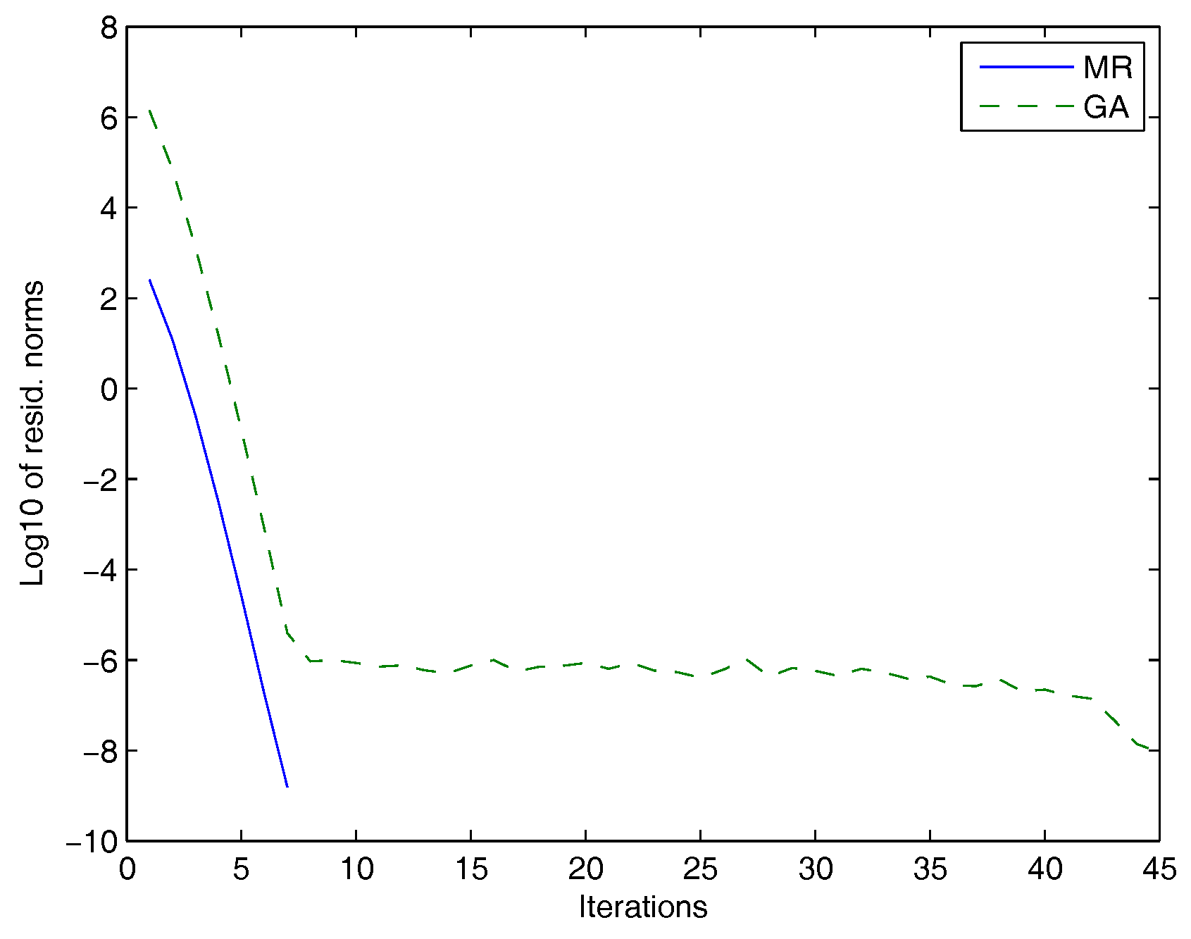
Example 2. For the second set of experiments, we considered matrices from the University of Florida Sparse Matrix Collection [31] and from the Harwell Boeing Collection (http://math.nist.gov/MatrixMarket). In
Figure 2, we used the matrices
A =
pde2961 and
B =
fdm with dimensions
and
, respectively, and
.
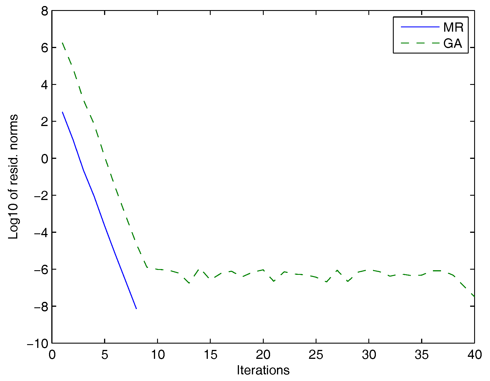
In
Figure 3, we used the matrices
A=
Themal and
B=
fdm with dimensions
and
, respectively, and
.
In
Table 2, we compared the performances of the MR method and the GA. For both methods, we listed the residual norms, the maximum number of iterations and the corresponding execution time.


