Deterministic Seirs Epidemic Model for Modeling Vital Dynamics, Vaccinations, and Temporary Immunity

Abstract

In this paper, the author proposes a new SEIRS model that generalizes several classical deterministic epidemic models (e.g., SIR and SIS and SEIR and SEIRS) involving the relationships between the susceptible S, exposed E, infected I, and recovered R individuals for understanding the proliferation of infectious diseases. As a way to incorporate the most important features of the previous models under the assumption of homogeneous mixing (mass-action principle) of the individuals in the population N, the SEIRS model utilizes vital dynamics with unequal birth and death rates, vaccinations for newborns and non-newborns, and temporary immunity. In order to determine the equilibrium points, namely the disease-free and endemic equilibrium points, and study their local stability behaviors, the SEIRS model is rescaled with the total time-varying population and analyzed according to its epidemic condition R₀ for two cases of no epidemic (R₀ ≤ 1) and epidemic (R₀ > 1) using the time-series and phase portraits of the susceptible s, exposed e, infected i, and recovered r individuals. Based on the experimental results using a set of arbitrarily-defined parameters for horizontal transmission of the infectious diseases, the proportional population of the SEIRS model consisted primarily of the recovered r (0.7–0.9) individuals and susceptible s (0.0–0.1) individuals (epidemic) and recovered r (0.9) individuals with only a small proportional population for the susceptible s (0.1) individuals (no epidemic). Overall, the initial conditions for the susceptible s, exposed e, infected i, and recovered r individuals reached the corresponding equilibrium point for local stability: no epidemic (DFE ${\overline{X}}_{DFE}$) and epidemic (EE ${\overline{X}}_{EE}$).

1. Introduction

Over the past decades, mathematical models have been developed and implemented to study the spread of infectious diseases since the early 20th century in the field of mathematical epidemiology [1,2,3,4]. The stochastic and deterministic epidemic models allow researchers to gain valuable insights into numerous infectious diseases and investigate strategies for combating them. For deterministic epidemic models, the populations of individuals are assigned to one of several different compartments, where each compartment represents a specific stage of the epidemic. The transition rates from one compartment to another compartment are mathematically expressed with derivatives. Based on the assorted compartments for the population and derivatives for the transition rates, the system of ordinary differential equations serves to describe the changes in population as a function of time.

From the seminal work in 1927, Kermack and McKendrick constructed a simple deterministic compartment model that still today acts as the fundamental model for developing and implementing even more complicated mathematical epidemic models [5]. In Kermack and McKendrick’s SIR classical compartmental model, the population N was divided into three compartments: susceptible S compartment, in which all the individuals are susceptible if they have contact with a disease; infected I compartment, in which all the individuals are infected by the disease and infectious to spread the disease; and recovered R compartment, in which all the individuals are recovered from the infection. For the SIR model, Kermack and McKendrick made three assumptions: (1) the disease spreads in a closed environment (i.e., no births or deaths) with constant population N; (2) the number of susceptibles S who are infected by an infected I individual per unit of time is proportional to the total number of susceptibles with the proportional (transmission) coefficient β, where total number of newly infectives is βSI; and (3) the number of recovered R individuals from the infected I compartment per unit time is γI, where γ is the recovery rate coefficient, with the recovered individuals gaining permanent immunity from the infectious disease. While the SIR model was accurate for describing the spread of viral diseases (e.g., influenza, measles, and chickenpox), the SIR model was inappropriate for dealing with bacterial diseases (e.g., encephalitis and gonorrhea), where the recovered individuals gained no immunity and could be re-infected by the disease again at a future time period. As a spinoff of the SIR model, Kermack and McKendrick proposed the SIS model 5 years later to study the dynamics of bacterial diseases [6]. In both the classical SIR and SIS models, the models assume a negligible disease incubation period, where the susceptible S individuals could become infected and later recovery to acquire permanent or temporary immunity.

For more general models than SIR and SIS models, the SEIR and SEIRS models assume that the susceptible S individuals—after infection—first proceed through the latent period as exposed E individuals before becoming infected I individuals and then eventually recovered R individuals [7,8]. In the exposed E compartment, the individuals are infected by the disease but do not have the visible symptoms of the disease and cannot communicate the disease to susceptible S individuals. In such a latent period, the disease takes a certain time for the infection to multiple inside the body of the susceptible S individuals to reach the critical level to become infected I individuals. After the incubation period of the disease, the exposed E individuals soon become infected I individuals and then either acquire permanent immunity (SEIR) or temporary immunity (SEIRS). As with the SIR and SIS models, the SEIR and SEIRS models assume homogeneous mixing (mass-action principle) of the individuals in the population.

With the SIR and SIS models along with the SEIR and SEIRS models, the models all assumed that the disease spreads in a closed environment. For such models, the population N is always a constant value since the models do not incorporate any births or deaths. In order to develop and implement more realistic mathematical models to mimic reality, Anderson and May investigated the use of vital dynamics to vary the size of the population [9,10]. By assuming a birth rate b and death rate d, the SEIR and SEIRS models with vital dynamics now have a time-varying population N(t) that more appropriately models the spread of the disease. Fundamentally, the total population increases by birth at a rate b and decreases at a rate of d. From the different compartments of susceptible S compartment, exposed E compartment, infected I compartment, and recovered R compartment, the total population N(t) adheres to the conversation law as the sum of the populations of the different compartments that all vary as a function of time.

In the presence of infectious diseases, the ideal goal is to fully eradicate them through either preventive measures or establishment of a mass immunization program. As an extension to the SEIR and SEIRS models with vital dynamics, Anderson and May studied vaccinations applied to newborns (i.e., babies) and non-newborns (i.e., children and adults) [11,12]. For mass immunization programs, newborns or susceptible S individuals receive the vaccines and proceed directly to the recovered R compartment. By providing the proper vaccines to the public, the mass immunization program serves to reduce the basic reproduction value R₀ to less than unity, which causes the infectious disease to die out eventually. For R₀ greater than unity, the infectious disease does not die out eventually and actually causes the occurrence of an epidemic. Due to successful immunization programs occasionally creating health problems to individuals since vaccinations offer some associated risks, the infected I individuals may become too fearful of the risks and then not receive the necessary vaccines until they have spread the infectious disease to many other susceptible S individuals. Before reaching an epidemic, legislation is sometimes passed to enforce vaccinations.

As a way to merge the significant features of the foundational and more advanced SIR and SIRS models [13,14] along with the SEIR and SEIRS models [15,16,17,18,19,20,21,22,23,24,25,26,27,28,29,30,31,32,33,34], the focus of the work is to develop and implement an extension of the SEIRS model. Fundamentally, the new SEIRS model is now a more advanced generalization of the previous models and incorporates vital dynamics with unequal birth and death rates, vaccinations for both newborns and non-newborns, and temporary immunity for describing the spread of infectious diseases. The SEIRS model with vital dynamics, vaccinations, and temporary immunity is rescaled using the total time-varying population and analyzed to determine its equilibrium points and corresponding local stabilities of the equilibrium points. In order to test the SEIRS model, numerical simulations are run involving a set of arbitrarily-defined parameters for horizontal transmission of the infectious disease in the new SEIRS model.

The remainder of this paper is organized into the following sections: epidemiological model (Section 2), local stability (Section 3), experimental methodology (Section 4), experimental results (Section 5), and conclusion (Section 6).

2. Epidemiological Model

In epidemiology, the new SEIRS model with vital dynamics (birth and death rates), vaccinations (newborns and non-newborns), and temporary immunity provides a mathematical description of infectious diseases and corresponding spread in biology. Figure 1 shows the block diagram of the SEIRS model with compartments (classes) consisting of susceptible S, exposed E, infected I, and recovered R individuals from the total population N.

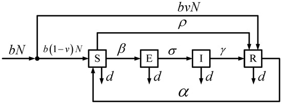
Figure 1. SEIRS Model with Vital Dynamics and Vaccinations.

The four classes of the model, S, E, I, R, are described in further detail in Table 1.

Table 1. Classes.

Parameter	Name	Units	Meaning
S	Susceptible Individuals	Number of Individuals	Individuals susceptible to infection who can contract the disease if they are exposed to it
E	Exposed Individuals	Number of Individuals	Individuals exposed to infection who are infected but have not yet become infectious and cannot pass the infection to other susceptible individuals
I	Infected Individuals	Number of Individuals	Individuals infected by infection who are capable of transmitting the infection to any susceptible individuals
R	Recovered Individuals	Number of Individuals	Individuals recovered from infection who are temporarily immune from the infection

For the SEIRS model, the model allows for vital dynamics with unequal birth and death rates, vaccinations of both newborns and non-newborns, and temporary immunity from the infectious disease. With the population, the newborns are all susceptible without vaccination. In specific terms, the newborns are not born with any maternally-derived immunity. At a later time period, the newborns (i.e., babies) who were not initially vaccinated and non-newborns (i.e., children and adults) who were not around during the inception of the infectious disease as newborns both compromise the susceptible class and have the ability to receive vaccines. Based on the interaction of susceptible individuals and infected individuals, the infectious disease transmission causes the susceptible individuals to now leave the susceptible class and enter the exposed class. After a specific time period, the incubating infection eventually causes the exposed individuals to obtain the infectious disease and then spread it to susceptible individuals. Without any vaccines to temporarily cure the exposed individuals and infected individuals, the infected individuals will recover from the infectious disease and enter the recovered class. Unfortunately, the recovered individuals experience only temporary immunity from the infectious disease and can potentially transition back into the susceptible class. Table 2 summarizes the interpretations of the different positive parameters embedded in the SEIRS model for each of the four classes.

Table 2. Description of Model Parameters.

Parameter	Name	Units	Meaning
b	Birth Rate	$\frac{\frac{\mathrm{births}}{\mathrm{person}}}{\mathrm{day}}$	Birth rate of newborns each year
d	Death Rate	$\frac{\frac{\mathrm{deaths}}{\mathrm{person}}}{\mathrm{day}}$	Death rate of susceptible, exposed, infected, and recovered individuals each year
ν	Vaccination Proportion (Newborns)	Dimensionless	Proportion of vaccinated newborns
ρ	Vaccination Rate (Susceptible)	days−1	Rate at which susceptible individuals are vaccinated and leave susceptible class and enter recovered class to gain temporary immunity
α	Transmission Rate (Recovered to Susceptible)	days−1	Rate at which recovered individuals lose temporary immunity and leave recovered class and enter susceptible class
β	Transmission Rate (Susceptible to Infected)	days−1	Rate at which susceptible individuals become exposed by infected individuals and leave susceptible class and enter exposed class
σ	Transmission Rate (Exposed to Infected)	days−1	Rate at which exposed individuals become infected by incubating infection and leave exposed class and enter infected class
γ	Recovery Rate (Infected to Recovered)	days−1	Rate at which infected individuals leave infected class and enter recovered class

From the positive parameters, the rates ρ (vaccination rate of non-newborns), α (transmission rate of recovered to susceptible), β (transmission rate of susceptible to infected), σ (transmission rate of exposed to infected), and γ (recovery rate of infected to recovered) are numerically interpreted in terms of their inverses. Table 3 explains the interpretations of the positive inverse parameters embedded in the SEIRS model.

Table 3. Description of Inverse Model Parameters.

Parameter	Name	Units	Meaning
$\frac{1}{\mathsf{\rho }}$	Mean Susceptibility Period (Pre-Vaccination of Susceptible Individuals)	days	Time for susceptible individuals to become recovered individuals
$\frac{1}{\mathsf{\alpha }}$	Mean Temporary Immunity Period	days	Time for recovered individuals to become susceptible individuals
$\frac{1}{\mathsf{\beta }}$	Mean Susceptibility Period (Pre-Exposed Individuals)	days	Time for susceptible individuals to become exposed individuals
$\frac{1}{\mathsf{\sigma }}$	Mean Latency Period	days	Time for exposed individuals to become infected individuals
$\frac{1}{\mathsf{\gamma }}$	Mean Infectious Period	days	Time for infected individuals to become recovered individuals

Based on the model parameters and inverse model parameters in Table 2 and Table 3, the SEIRS model is transformed into mathematical system for analysis and evaluation.

Mathematically, the SEIRS model is expressed as a system of ordinary differential equations given as:

$$\begin{array}{l}\frac{dS}{dt}=b\left(1-\mathsf{\nu }\right)N-\mathsf{\beta }\frac{SI}{N}-dS+\mathsf{\alpha }R-\mathsf{\rho }S\\ \frac{dE}{dt}=\mathsf{\beta }\frac{SI}{N}-\mathsf{\sigma }E-dE\\ \frac{dI}{dt}=\mathsf{\sigma }E-\mathsf{\gamma }I-dI\\ \frac{dR}{dt}=b\mathsf{\nu }N+\mathsf{\gamma }I-dR-\mathsf{\alpha }R+\mathsf{\rho }S\end{array}$$

(1)

with population:

$$S\left(t\right)+E\left(t\right)+I\left(t\right)+R\left(t\right)=N\left(t\right)$$

(2)

or:

$$S^{\prime }\left(t\right)+E^{\prime }\left(t\right)+I^{\prime }\left(t\right)+R^{\prime }\left(t\right)=N^{\prime }\left(t\right)=\frac{dN}{dt}$$

(3)

where $\mathsf{\beta }\frac{SI}{N}$ is the incidence rate at which the susceptible S become infected I by a disease. By substitution of the ordinary differential equation system in (1) into the relationship of (3), the population N is governed by the ordinary differential equation:

$$\frac{dN}{dt}=\left(b-d\right)N$$

(4)

Since (4) does not depend on any of the other variables in the system in (1), the population N is computed using separation of variables:

$$\frac{1}{N}dN=\left(b-d\right)dt$$

(5)

or:

$${\displaystyle \int \frac{1}{N}dN}=\left(b-d\right){\displaystyle \int dt}$$

(6)

to yield:

$$\ln \left(N\right)=\left(b-d\right)t$$

(7)

As a result of solving (7) through exponentiation, the population N is given as:

$$N=e^{\left(b-d\right)t}$$

(8)

with time-varying population N(t).

Instead of solving the ordinary differential equation system in (1) with known population N from (8), the transformations:

$$s=\frac{S}{N}$$

(9)

and:

$$e=\frac{E}{N}$$

(10)

and:

$$i=\frac{I}{N}$$

(11)

and:

$$r=\frac{R}{N}$$

(12)

are applied to the system in (1), where s, e, i, and r denote the fractions of the number of individuals in classes S, E, I, and R with population N. Now, the transformed system (see Appendix A for more details) is formulated as:

$$\begin{array}{l}\frac{ds}{dt}=b\left(1-\mathsf{\nu }\right)-\mathsf{\beta }si+\mathsf{\alpha }r-\left(b+\mathsf{\rho }\right)s\\ \frac{de}{dt}=\mathsf{\beta }si-\left(b+\mathsf{\sigma }\right)e\\ \frac{di}{dt}=\mathsf{\sigma }e-\left(b+\mathsf{\gamma }\right)i\\ \frac{dr}{dt}=b\mathsf{\nu }+\mathsf{\gamma }i+\mathsf{\rho }s-\left(b+\mathsf{\alpha }\right)r\end{array}$$

(13)

which is equivalent to the system in (1). By substitution of the transformations in (9)–(12), (2) is written as:

$$s+e+i+r=1$$

(14)

or:

$$s^{\prime }+e^{\prime }+i^{\prime }+r^{\prime }=0$$

(15)

With manipulation of (14) to produce:

$$r=1-s-e-i$$

(16)

(16) is substituted into the transformed system in (13) to eliminate r and yield the simplified subsystem:

$$\begin{array}{l}\frac{ds}{dt}=\mathsf{\alpha }+b\left(1-\mathsf{\nu }\right)-\mathsf{\alpha }e-\mathsf{\alpha }i-\mathsf{\beta }si-\left(b+\mathsf{\rho }+\mathsf{\alpha }\right)s\\ \frac{de}{dt}=\mathsf{\beta }si-\left(b+\mathsf{\sigma }\right)e\\ \frac{di}{dt}=\mathsf{\sigma }e-\left(b+\mathsf{\gamma }\right)i\end{array}$$

(17)

or:

$$\begin{array}{l}\frac{ds}{dt}=A-\mathsf{\alpha }e-\mathsf{\alpha }i-\mathsf{\beta }si-Bs\\ \frac{de}{dt}=\mathsf{\beta }si-Ce\\ \frac{di}{dt}=\mathsf{\sigma }e-Di\end{array}$$

(18)

with positive constants:

$$A=\mathsf{\alpha }+b\left(1-\mathsf{\nu }\right)$$

(19)

$$B=b+\mathsf{\rho }+\mathsf{\alpha }$$

(20)

$$C=b+\mathsf{\sigma }$$

(21)

and:

$$D=b+\mathsf{\gamma }$$

(22)

Based on the solutions of the subsystem in (18), s, e, and i are utilized to solve for r in:

$$\frac{dr}{dt}=b\mathsf{\nu }+\mathsf{\gamma }i+\mathsf{\rho }s-Fr$$

(23)

or (16), where:

$$F=b+\mathsf{\alpha }$$

(24)

is a positive constant. In order to transform the system in (13) back to the original system in (1), the solutions s, e, i, and r and N in (8) are inserted into the transformations in (9)–(12).

3. Local Stability

From the transformed subsystem in (18), the local stability is analyzed to determine the disease-free equilibrium (DFE):

$${\overline{X}}_{DFE}=\left(s,e,i\right)=\left(s^{\ast },0,0\right)$$

(25)

and endemic equilibrium (EE):

$${\overline{X}}_{EE}=\left(s,e,i\right)=\left(s^{\ast },e^{\ast },i^{\ast }\right)$$

(26)

Specifically, the equilibrium points are computed by setting $\frac{ds}{dt}=0$, $\frac{de}{dt}=0$, and $\frac{di}{dt}=0$ and solving for s, e, and i in (18) to compute the two equilibrium points. From the equilibrium points, the Jacobian matrix J is calculated from:

$$\left[\begin{array}{c}G\\ H\\ K\end{array}\right]=\left[\begin{array}{c}ds/dt\\ de/dt\\ di/dt\end{array}\right]=\left[\begin{array}{c}A-\mathsf{\alpha }e-\mathsf{\alpha }i-\mathsf{\beta }si-Bs\\ \mathsf{\beta }si-Ce\\ \mathsf{\sigma }e-Di\end{array}\right]$$

(27)

as:

$$J\left(X\right)=J\left(s,e,i\right)=\left[\begin{array}{ccc}\partial G/\partial s& \partial G/\partial e& \partial G/\partial i\\ \partial H/\partial s& \partial H/\partial e& \partial H/\partial i\\ \partial K/\partial s& \partial K/\partial e& \partial K/\partial i\end{array}\right]=\left[\begin{array}{ccc}-\mathsf{\beta }i-B& -\mathsf{\alpha }& -\mathsf{\alpha }-\mathsf{\beta }s\\ \mathsf{\beta }i& -C& \mathsf{\beta }s\\ 0& \mathsf{\sigma }& -D\end{array}\right]$$

(28)

and evaluated at the equilibrium points to decide on the local stability, which is directly determined from the eigenvalues λ of:

$$\left|J\left(X\right)-\mathsf{\lambda }I\right|=0$$

(29)

Based on the eigenvalues λ of (29), the linearized system will either be stable (all the eigenvalues of the Jacobian evaluated at the equilibrium point contain negative real parts) or unstable (at least one of the eigenvalues of the Jacobian evaluated at the equilibrium point has positive real part) for the transformed subsystem in (18).

3.1. Disease-Free Equilibrium

Through substitution of (25) into $\frac{ds}{dt}=0$ of the transformed subsystem in (18), the DFE ${\overline{X}}_{DFE}$ in (25) is computed as:

$${\frac{ds}{dt}|}_{{\overline{X}}_{DFE}}=0={\left(A-\mathsf{\alpha }e-\mathsf{\alpha }i-\mathsf{\beta }si-Bs\right)|}_{{\overline{X}}_{DFE}}$$

(30)

to generate:

$$s=\frac{A}{B}$$

(31)

or:

$${\overline{X}}_{DFE}=\left(s,e,i\right)=\left(s^{\ast },0,0\right)=\left(\frac{A}{B},0,0\right)$$

(32)

At the DFE ${\overline{X}}_{DFE}=\left(\frac{A}{B},0,0\right)$, the Jacobian matrix J(X) in (28) is given as:

$$J\left({\overline{X}}_{DFE}\right)=\left[\begin{array}{ccc}-B& -\mathsf{\alpha }& -\mathsf{\alpha }-\mathsf{\beta }\frac{A}{B}\\ 0& -C& \mathsf{\beta }\frac{A}{B}\\ 0& \mathsf{\sigma }& -D\end{array}\right]$$

(33)

with eigenvalues λ:

$$\left|J\left({\overline{X}}_{DFE}\right)-\mathsf{\lambda }I\right|=0$$

(34)

or:

$$\left|\begin{array}{ccc}-B-\mathsf{\lambda }& -\mathsf{\alpha }& -\mathsf{\alpha }-\mathsf{\beta }\frac{A}{B}\\ 0& -C-\mathsf{\lambda }& \mathsf{\beta }\frac{A}{B}\\ 0& \mathsf{\sigma }& -D-\mathsf{\lambda }\end{array}\right|=0$$

(35)

which is expanded as:

$$\left(-B-\mathsf{\lambda }\right)\left|\begin{array}{cc}-C-\mathsf{\lambda }& \mathsf{\beta }\frac{A}{B}\\ \mathsf{\sigma }& -D-\mathsf{\lambda }\end{array}\right|+\mathsf{\alpha }\left|\begin{array}{cc}0& \mathsf{\beta }\frac{A}{B}\\ 0& -D-\mathsf{\lambda }\end{array}\right|+\left(-\mathsf{\alpha }-\mathsf{\beta }\frac{A}{B}\right)\left|\begin{array}{cc}0& -C-\mathsf{\lambda }\\ 0& \mathsf{\sigma }\end{array}\right|=0$$

(36)

By evaluating the determinants in (36), the eigenvalues λ are determined from the cubic polynomial:

$$P\left(\mathsf{\lambda }\right)={\mathsf{\lambda }}^3+\left(B+C+D\right){\mathsf{\lambda }}^2+\left(BC+BD+CD-\mathsf{\sigma }\mathsf{\beta }\frac{A}{B}\right)\mathsf{\lambda }+\left(BCD-\mathsf{\sigma }\mathsf{\beta }A\right)=0$$

(37)

where the three eigenvalues λ are dependent on the parameters σ and β and constants A, B, C, and D.

Unfortunately, the eigenvalues λ are difficult to compute for the cubic polynomial in (37) without any specific values for the parameters σ and β and constants A, B, C, and D. In order to determine the parameter and constant independent local stability of the DFE ${\overline{X}}_{DFE}$ in (25), the Routh-Hurwitz criteria is applied to the cubic polynomial in (37) with the coefficients:

$$a_1=B+C+D$$

(38)

$$a_2=BC+BD+CD-\mathsf{\sigma }\mathsf{\beta }\frac{A}{B}$$

(39)

and:

$$a_3=BCD-\mathsf{\sigma }\mathsf{\beta }A$$

(40)

Based on the Routh-Hurwitz criteria for a cubic polynomial P(λ), the three conditions:

$$a_1>0$$

(41)

$$a_3>0$$

(42)

and:

$$a_1{a}_2>a_3$$

(43)

must satisfied for the DFE ${\overline{X}}_{DFE}$ in (25) to be locally stable. For the first condition (41):

$$a_1=B+C+D>0$$

(44)

since the constants $B>0$, $C>0$, and $D>0$ in (20)–(22). With the second condition (42):

$$a_3=BCD-\mathsf{\sigma }\mathsf{\beta }A>0$$

(45)

if:

$$\frac{BCD}{\mathsf{\sigma }\mathsf{\beta }A}>1$$

(46)

From the third condition (43):

$$a_1{a}_2=\left(B+C+D\right)\left(BC+BD+CD-\mathsf{\sigma }\mathsf{\beta }\frac{A}{B}\right)$$

(47)

or:

$$a_1{a}_2=B^{2}C+B^{2}D+3BCD+B{C}^2+C^{2}D+B{D}^2+C{D}^2-\mathsf{\sigma }\mathsf{\beta }A-\mathsf{\sigma }\mathsf{\beta }\frac{AC}{B}-\mathsf{\sigma }\mathsf{\beta }\frac{AD}{B}$$

(48)

By cancellation of BCD and −σβA in (45) and (48), (43) is simplified as:

$$B^{2}C+B^{2}D+2BCD+B{C}^2+C^{2}D+B{D}^2+C{D}^2-\mathsf{\sigma }\mathsf{\beta }\frac{AC}{B}-\mathsf{\sigma }\mathsf{\beta }\frac{AD}{B}>0$$

(49)

or:

$$B^{2}C+B^{2}D+2BCD+B{C}^2+C^{2}D+B{D}^2+C{D}^2>\frac{\mathsf{\sigma }\mathsf{\beta }A}{B}\left(C+D\right)$$

(50)

After dividing by $BC$, (50) is simplified as:

$$\left(\frac{B^2}{D}+\frac{B^2}{C}+2B+\frac{BC}{D}+\frac{BD}{C}\right)+1\left(C+D\right)>\frac{\mathsf{\sigma }\mathsf{\beta }A}{BCD}\left(C+D\right)$$

(51)

where:

$$\frac{\mathsf{\sigma }\mathsf{\beta }A}{BCD}\le 1$$

(52)

As a result of the Routh-Hurwitz criteria, all the eigenvalues λ in the cubic polynomial P(λ) in (37) have negative real parts to conclude that the DFE ${\overline{X}}_{DFE}$ in (25) is locally stable with (46).

3.2. Endemic Equilibrium

From the transformed subsystem in (18), the EE ${\overline{X}}_{EE}$ in (26) is computed by developing a relationship between i and e through $\frac{di}{dt}=0$ as:

$$\frac{di}{dt}=0=\mathsf{\sigma }e-Di$$

(53)

or:

$$i=\frac{\mathsf{\sigma }}{D}e$$

(54)

where:

$$\frac{e}{i}=\frac{D}{\mathsf{\sigma }}$$

(55)

By examining $\frac{de}{dt}=0$ as:

$$\frac{de}{dt}=0=\mathsf{\beta }si-Ce$$

(56)

or:

$$s=\frac{C}{\mathsf{\beta }}\frac{e}{i}$$

(57)

(55) is substituted into (57) to deliver the first coordinate of EE ${\overline{X}}_{EE}$ as:

$$s=\frac{CD}{\mathsf{\beta }\mathsf{\sigma }}$$

(58)

With $\frac{ds}{dt}=0$ as:

$$\frac{ds}{dt}=0=A-\mathsf{\alpha }e-\mathsf{\alpha }i-\mathsf{\beta }si-Bs$$

(59)

or:

$$s\left(\mathsf{\beta }i+B\right)=A-\mathsf{\alpha }e-\mathsf{\alpha }i$$

(60)

(58) is inserted into (60) as:

$$\left(\frac{CD}{\mathsf{\beta }\mathsf{\sigma }}\right)\left(\mathsf{\beta }i+B\right)=A-\mathsf{\alpha }e-\mathsf{\alpha }i$$

(61)

After distributing and collecting terms in (61):

$$i\left(\frac{CD}{\mathsf{\sigma }}+\mathsf{\alpha }\right)=A-\mathsf{\alpha }e-\frac{BCD}{\mathsf{\beta }\mathsf{\sigma }}$$

(62)

which is further simplified with (54) as:

$$\left(\frac{\mathsf{\sigma }}{D}e\right)\left(\frac{CD}{\mathsf{\sigma }}+\mathsf{\alpha }\right)=A-\mathsf{\alpha }e-\frac{BCD}{\mathsf{\beta }\mathsf{\sigma }}$$

(63)

or:

$$e\left[\left(\frac{\mathsf{\sigma }}{D}\right)\left(\frac{CD}{\mathsf{\sigma }}+\mathsf{\alpha }\right)+\mathsf{\alpha }\right]=A-\frac{BCD}{\mathsf{\beta }\mathsf{\sigma }}$$

(64)

By distributing and combining fractions, (64) is written as:

$$e\left[C+\frac{\mathsf{\alpha }\mathsf{\sigma }}{D}+\mathsf{\alpha }\right]=A-\frac{BCD}{\mathsf{\beta }\mathsf{\sigma }}$$

(65)

or:

$$e\left[\frac{CD+\mathsf{\alpha }\mathsf{\sigma }+\mathsf{\alpha }D}{D}\right]=\frac{\mathsf{\beta }\mathsf{\sigma }A-BCD}{\mathsf{\beta }\mathsf{\sigma }}$$

(66)

to supply the second coordinate of EE ${\overline{X}}_{EE}$ as:

$$e=\left(\frac{D}{CD+\mathsf{\alpha }\mathsf{\sigma }+\mathsf{\alpha }D}\right)\left(\frac{\mathsf{\beta }\mathsf{\sigma }A-BCD}{\mathsf{\beta }\mathsf{\sigma }}\right)$$

(67)

Through substitution of (67) into (54), the third coordinate of the EE ${\overline{X}}_{EE}$ is given as:

$$i=\frac{\mathsf{\beta }\mathsf{\sigma }A-BCD}{\mathsf{\beta }\left(CD+\mathsf{\alpha }\mathsf{\sigma }+\mathsf{\alpha }D\right)}$$

(68)

With (58), (67), and (68), the EE ${\overline{X}}_{EE}$ in (26) is given by:

$${\overline{X}}_{EE}=\left(s,e,i\right)=\left(s^{\ast },e^{\ast },i^{\ast }\right)=\left(\frac{CD}{\mathsf{\beta }\mathsf{\sigma }},\left(\frac{D}{CD+\mathsf{\alpha }\mathsf{\sigma }+\mathsf{\alpha }D}\right)\left(\frac{\mathsf{\beta }\mathsf{\sigma }A-BCD}{\mathsf{\beta }\mathsf{\sigma }}\right),\frac{\mathsf{\beta }\mathsf{\sigma }A-BCD}{\mathsf{\beta }\left(CD+\mathsf{\alpha }\mathsf{\sigma }+\mathsf{\alpha }D\right)}\right)$$

(69)

which only makes physical sense if:

$$\mathsf{\beta }\mathsf{\sigma }A-BCD>0$$

(70)

since all the constants A, B, C, and D and parameters α, β, and σ in (69) are positive values. By manipulating the inequality in (70), the epidemic condition R₀ is given as:

$$R_0=\frac{\mathsf{\beta }\mathsf{\sigma }A}{BCD}>1$$

(71)

The epidemic condition R₀ in (71) is the basic reproduction value and is the most important quantity to consider for analyzing any epidemiological model. In particular, R₀ determines whether an epidemic occurs for infectious diseases since R₀ is the average number of secondary infections produced by one infected individual during the mean period of infection in a fully susceptible population. If R₀ ≤ 1, then, on average, the number of new infections produced by one infected individual over the mean course of the infectious disease is less than unity, which implies the infectious disease dies out eventually. Conversely, if R₀ > 1, then, on average, the number of new infections produced by one infected individual is greater than unity, which leads to the persistence of the infectious disease as an epidemic. At the EE ${\overline{X}}_{EE}$ in (69), the Jacobian matrix J(X) is given by:

$$J\left({\overline{X}}_{EE}\right)=\left[\begin{array}{ccc}-\mathsf{\beta }{i}^{\ast }-B& -\mathsf{\alpha }& -\mathsf{\alpha }-\mathsf{\beta }{s}^{\ast }\\ \mathsf{\beta }{i}^{\ast }& -C& \mathsf{\beta }{s}^{\ast }\\ 0& \mathsf{\sigma }& -D\end{array}\right]$$

(72)

with eigenvalues λ:

$$\left|J\left({\overline{X}}_{EE}\right)-\mathsf{\lambda }I\right|=0$$

(73)

or:

$$\left|\begin{array}{ccc}-\mathsf{\beta }{i}^{\ast }-B& -\mathsf{\alpha }& -\mathsf{\alpha }-\mathsf{\beta }{s}^{\ast }\\ \mathsf{\beta }{i}^{\ast }& -C& \mathsf{\beta }{s}^{\ast }\\ 0& \mathsf{\sigma }& -D\end{array}\right|=0$$

(74)

which is expanded as:

$$\left(-\mathsf{\beta }{i}^{\ast }-B-\mathsf{\lambda }\right)\left|\begin{array}{cc}-C-\mathsf{\lambda }& \mathsf{\beta }{s}^{\ast }\\ \mathsf{\sigma }& -D-\mathsf{\lambda }\end{array}\right|+\mathsf{\alpha }\left|\begin{array}{cc}\mathsf{\beta }{i}^{\ast }& -C-\mathsf{\lambda }\\ 0& \mathsf{\sigma }\end{array}\right|+\left(-\mathsf{\alpha }-\mathsf{\beta }{i}^{\ast }\right)\left|\begin{array}{cc}\mathsf{\beta }{i}^{\ast }& -C-\mathsf{\lambda }\\ 0& \mathsf{\sigma }\end{array}\right|=0$$

(75)

Through evaluation of the determinants in (75), the eigenvalues λ are computed from the cubic polynomial:

$$\begin{array}{r}P\left(\mathsf{\lambda }\right)={\mathsf{\lambda }}^3+\left(B+C+D+\mathsf{\beta }{i}^{\ast }\right){\mathsf{\lambda }}^2+\left(BC+BD+CD+\mathsf{\beta }C{i}^{\ast }+\mathsf{\beta }D{i}^{\ast }-\mathsf{\sigma }\mathsf{\beta }{s}^{\ast }\right)\mathsf{\lambda }\\ +\left(BCD+\mathsf{\beta }CD{i}^{\ast }-\mathsf{\sigma }\mathsf{\beta }B{s}^{\ast }\right)=0\end{array}$$

(76)

or:

$$\begin{array}{r}P\left(\mathsf{\lambda }\right)={\mathsf{\lambda }}^3+\left(B+C+D+\frac{\mathsf{\beta }\mathsf{\sigma }A-BCD}{CD+\mathsf{\alpha }\mathsf{\sigma }+\mathsf{\alpha }D}\right){\mathsf{\lambda }}^2+\left(BC+BD+C\left(\frac{\mathsf{\beta }\mathsf{\sigma }A-BCD}{CD+\mathsf{\alpha }\mathsf{\sigma }+\mathsf{\alpha }D}\right)+D\left(\frac{\mathsf{\beta }\mathsf{\sigma }A-BCD}{CD+\mathsf{\alpha }\mathsf{\sigma }+\mathsf{\alpha }D}\right)\right)\mathsf{\lambda }\\ +\left(CD\left(\frac{\mathsf{\beta }\mathsf{\sigma }A-BCD}{CD+\mathsf{\alpha }\mathsf{\sigma }+\mathsf{\alpha }D}\right)\right)=0\end{array}$$

(77)

where the three eigenvalues λ are dependent on the parameters σ and β, constants A, B, C, and D, and first and third coordinates of EE ${\overline{X}}_{EE}$, namely s* and i* in (69).

In a similar manner to the eigenvalues λ for the cubic polynomial in (37), the eigenvalues λ for the cubic polynomial in (77) are even more difficult to compute without any specific values for the parameters σ and β and constants A, B, C, and D. The Routh-Hurwitz criteria with conditions (41)–(43) is again applied to now the cubic polynomial in (77) to determine the parameter and constant independent local stability of the EE ${\overline{X}}_{EE}$ in (69) with the coefficients:

$$\begin{array}{cc}{a}_1& =B+C+D+\frac{\mathsf{\beta }\mathsf{\sigma }A-BCD}{CD+\mathsf{\alpha }\mathsf{\sigma }+\mathsf{\alpha }D}\hfill \\ & =\frac{\mathsf{\alpha }\mathsf{\sigma }B+\mathsf{\alpha }BD+C^{2}D+\mathsf{\alpha }\mathsf{\sigma }C+\mathsf{\alpha }CD+C{D}^2+\mathsf{\alpha }\mathsf{\sigma }D+\mathsf{\alpha }{D}^2+\mathsf{\beta }\mathsf{\sigma }A}{CD+\mathsf{\alpha }\mathsf{\sigma }+\mathsf{\alpha }D}\hfill \end{array}$$

(78)

$$\begin{array}{cc}{a}_2& =BC+BD+C\left(\frac{\mathsf{\beta }\mathsf{\sigma }A-BCD}{CD+\mathsf{\alpha }\mathsf{\sigma }+\mathsf{\alpha }D}\right)+D\left(\frac{\mathsf{\beta }\mathsf{\sigma }A-BCD}{CD+\mathsf{\alpha }\mathsf{\sigma }+\mathsf{\alpha }D}\right)\hfill \\ & =\frac{\mathsf{\alpha }\mathsf{\sigma }BC+\mathsf{\alpha }\mathrm{B}CD+\mathsf{\alpha }\mathsf{\sigma }BD+\mathsf{\alpha }B{D}^2+\mathsf{\beta }\mathsf{\sigma }AC+\mathsf{\beta }\mathsf{\sigma }AD}{CD+\mathsf{\alpha }\mathsf{\sigma }+\mathsf{\alpha }D}\hfill \end{array}$$

(79)

and:

$$a_3=CD\left(\frac{\mathsf{\beta }\mathsf{\sigma }A-BCD}{CD+\mathsf{\alpha }\mathsf{\sigma }+\mathsf{\alpha }D}\right)=\frac{\mathsf{\beta }\mathsf{\sigma }ACD-B{C}^2{D}^2}{CD+\mathsf{\alpha }\mathsf{\sigma }+\mathsf{\alpha }D}$$

(80)

From the first condition (41):

$$a_1=\frac{\mathsf{\alpha }\mathsf{\sigma }B+\mathsf{\alpha }BD+C^{2}D+\mathsf{\alpha }\mathsf{\sigma }C+\mathsf{\alpha }CD+C{D}^2+\mathsf{\alpha }\mathsf{\sigma }D+\mathsf{\alpha }{D}^2+\mathsf{\beta }\mathsf{\sigma }A}{CD+\mathsf{\alpha }\mathsf{\sigma }+\mathsf{\alpha }D}>0$$

(81)

since the constants A > 0, B > 0, C > 0, and D > 0 and parameters α >0, β > 0, σ > 0 in (20)–(22) and Table. With the second condition (42):

$$a_3=\frac{\mathsf{\beta }\mathsf{\sigma }ACD-B{C}^2{D}^2}{CD+\mathsf{\alpha }\mathsf{\sigma }+\mathsf{\alpha }D}>0$$

(82)

or:

$$a_3=\mathsf{\beta }\mathsf{\sigma }A-BCD>0$$

(83)

if (71). For the third condition (43):

$$a_1{a}_2=\frac{\left(\mathsf{\alpha }\mathsf{\sigma }B+\mathsf{\alpha }BD+C^{2}D+\mathsf{\alpha }\mathsf{\sigma }C+\mathsf{\alpha }CD+C{D}^2+\mathsf{\alpha }\mathsf{\sigma }D+\mathsf{\alpha }{D}^2+\mathsf{\beta }\mathsf{\sigma }A\right)\left(\mathsf{\alpha }\mathsf{\sigma }BC+\mathsf{\alpha }BCD+\mathsf{\alpha }\mathsf{\sigma }BD+\mathsf{\alpha }B{D}^2+\mathsf{\beta }\mathsf{\sigma }AC+\mathsf{\beta }\mathsf{\sigma }AD\right)}{{\left(CD+\mathsf{\alpha }\mathsf{\sigma }+\mathsf{\alpha }D\right)}^2}$$

(84)

Through multiplication of (83) and (84) by (CD + ασ + αD)², (43) is simplified as:

$$\begin{array}{l}\left(\mathsf{\alpha }\mathsf{\sigma }B+\mathsf{\alpha }BD+C^{2}D+\mathsf{\alpha }\mathsf{\sigma }C+\mathsf{\alpha }CD+C{D}^2+\mathsf{\alpha }\mathsf{\sigma }D+\mathsf{\alpha }{D}^2+\mathsf{\beta }\mathsf{\sigma }A\right)\left(\mathsf{\alpha }\mathsf{\sigma }BC+\mathsf{\alpha }BCD+\mathsf{\alpha }\mathsf{\sigma }BD+\mathsf{\alpha }B{D}^2+\mathsf{\beta }\mathsf{\sigma }AC+\mathsf{\beta }\mathsf{\sigma }AD\right)\\ >\left(CD+\mathsf{\alpha }\mathsf{\sigma }+\mathsf{\alpha }D\right)\left(\mathsf{\beta }\mathsf{\sigma }ACD-B{C}^2{D}^2\right)\end{array}$$

(85)

or:

$$\begin{array}{l}{\mathsf{\alpha }}^2{B}^2{D}^3+{\mathsf{\alpha }}^{2}B{D}^4+{\mathsf{\alpha }}^2{\mathsf{\sigma }}^2{B}^{2}C+{\mathsf{\alpha }}^2{\mathsf{\sigma }}^2{B}^{2}D\\ +2{\mathsf{\alpha }}^2\mathsf{\sigma }{B}^2{D}^2+3\mathsf{\alpha }B{C}^2{D}^3+{\mathsf{\alpha }}^2{\mathsf{\sigma }}^{2}B{C}^2+{\mathsf{\alpha }}^2{\mathsf{\sigma }}^{2}A{C}^2\\ +2{\mathsf{\alpha }}^{2}BC{D}^3+\mathsf{\alpha }BC{D}^4+{\mathsf{\alpha }}^2{\mathsf{\sigma }}^{2}B{D}^2+2{\mathsf{\alpha }}^2\mathsf{\sigma }B{D}^3\\ +{\mathsf{\beta }}^2{\mathsf{\sigma }}^2{A}^{2}D+{\mathsf{\alpha }}^2{B}^{2}C{D}^2+\mathsf{\alpha }B{C}^3{D}^2+{\mathsf{\alpha }}^{2}B{C}^2{D}^2\\ +{\mathsf{\alpha }}^2{\mathsf{\sigma }}^{2}ABC+2{\mathsf{\alpha }}^2\mathsf{\sigma }{B}^{2}CD+\mathsf{\alpha }\mathsf{\sigma }B{C}^{3}D\\ +3\mathsf{\alpha }\mathsf{\sigma }B{C}^2{D}^2+\mathsf{\alpha }\mathsf{\sigma }A{C}^{3}D+2{\mathsf{\alpha }}^2{\mathsf{\sigma }}^{2}BCD\\ +4{\mathsf{\alpha }}^2\mathsf{\sigma }BC{D}^2+2{\mathsf{\alpha }}^2\mathsf{\sigma }B{C}^{2}D+{\mathsf{\alpha }}^2\mathsf{\sigma }A{C}^{2}D\\ +\mathsf{\alpha }\mathsf{\sigma }BC{D}^3+\mathsf{\alpha }\mathsf{\sigma }A{C}^2{D}^2+\mathsf{\beta }\mathsf{\sigma }AC{D}^3+{\mathsf{\alpha }}^2{\mathsf{\sigma }}^{2}ACD\\ +{\mathsf{\alpha }\mathsf{\beta }\mathsf{\sigma }}^{2}A{D}^2+{\mathsf{\alpha }}^2\mathsf{\sigma }AC{D}^2+\mathsf{\alpha }\mathsf{\beta }\mathsf{\sigma }A{D}^3+{\mathsf{\alpha }\mathsf{\sigma }}^2\mathsf{\beta }{A}^{2}C\\ +{\mathsf{\alpha }\mathsf{\beta }\mathsf{\sigma }}^{2}ABC+2{\mathsf{\alpha }\mathsf{\sigma }}^2\mathsf{\beta }ABD+{\mathsf{\alpha }}^2\mathsf{\sigma }ABCD\\ +2\mathsf{\alpha }\mathsf{\beta }\mathsf{\sigma }AB{D}^2+\mathsf{\alpha }\mathsf{\beta }\mathsf{\sigma }ABCD+B{C}^3{D}^3\\ >0\end{array}$$

(86)

As a consequence of the Routh-Hurwitz criteria, all the eigenvalues λ in the cubic polynomial P(λ) in (77) have negative real parts to conclude that the DFE ${\overline{X}}_{EE}$ in (69) is locally stable with (71).

4. Experimental Methodology

The proposed SEIRS model with vital dynamics, vaccinations, temporary immunity developed in (1) and transformed to the subsystem of ordinary differential equations in (18) was evaluated in Matlab. Table 4 lists a typical set of numerical values for the model parameters and inverse model parameters for all the experiments.

Table 4. Numerical Values of Model Parameters and Inverse Model Parameters.

Parameter	Value
b	$\frac{\frac{1.9}{100}}{365}\frac{\frac{\mathrm{births}}{\mathrm{person}}}{\mathrm{day}}$
d	$\frac{\frac{0.8}{100}}{365}\frac{\frac{\mathrm{births}}{\mathrm{person}}}{\mathrm{day}}$
ν	0.8
$\frac{1}{\mathsf{\rho }}$	2 days
$\frac{1}{\mathsf{\alpha }}$	14 days
$\frac{1}{\mathsf{\beta }}$	4 days (No Epidemic)	¼ days (Epidemic)
$\frac{1}{\mathsf{\sigma }}$	3 days
$\frac{1}{\mathsf{\gamma }}$	7 days

Based on the numerical values of the model parameters and inverse model parameters, the positive constants A, B, C, D and F ((19)–(22) and (24)) along with the epidemic condition R₀ ((71)) are computed for the SEIRS model in (18) and shown in Table 5.

Table 5. Constants.

Parameter	Value
$A$	0.07140
$B$	0.57150
$C$	0.33340
$D$	0.14290
$F$	0.07150
$R_0$	0.21865 (No Epidemic)	3.49840 (Epidemic)

For the SEIRS model in (18) with rescaled variables s, e, i, and r ((9)–(12)), the total population n is assumed to have a value of unity ((14)), where the population N of the original SEIRS model in (1) is assumed to have a value of 100 ((2)).

5. Experimental Results

Simulations were performed using the proposed and rescaled SEIRS model with vital dynamics, vaccinations, and temporary immunity in (18) along with the numerical values of the model parameters and inverse model parameters (Table 4) and constants (Table 5). In order to differentiate between the possibilities for the epidemic condition R₀, the two cases of no epidemic (R₀ ≤ 1) and epidemic (R₀ > 1) were analyzed separately. For both the no epidemic and epidemic cases, the local stability of the DFE ${\overline{X}}_{DFE}$ and EE ${\overline{X}}_{EE}$ equilibrium points in (32) and (69) were evaluated using their corresponding eigenvalues λ_i from their specific Jacobian matrix $J\left(\overline{X}\right)$. The proportional population of the rescaled variables s, e, i, and r with total population n of unity was studied through the subsequent time-series with various initial conditions s(0), e(0), i(0) and r(0) over the course of a 90-day period. As a way to examine the relationships between the different rescaled variables, phase portraits were utilized to trace the solution of the system of ordinary differential equations for the rescaled SEIRS model in (18). With all of the numerical simulations, the time period is assumed to have units of days.

5.1. No Epidemic

Based on the numerical values of the model and inverse model parameters and constants with β = 1/4 (0.25 susceptible individuals who become exposed by infected individuals and leave the susceptible class and enter the exposed class per day) for the rescaled SEIRS model in (18), the epidemic condition R₀ was calculated as R₀ = 0.21865, which is less than unity and implies no epidemic for the infectious disease. Table 6 shows the DFE and EE equilibrium points ${\overline{X}}_{DFE}$ and ${\overline{X}}_{EE}$ and eigenvalues λ_i of the Jacobian matrices $J\left({\overline{X}}_{DFE}\right)$ and $J\left({\overline{X}}_{EE}\right)$ along with their local stabilities.

Table 6. Local Stability (β = ¼ (No Epidemic)).

Point	s	e	i	λ1	λ2	λ3	Stability
DFE	0.12501	0	0	−0.57148	−0.37775	−0.09855	Stable
EE	0.57173	−0.44677	−1.0421	−0.44276 +i0.14310	−0.44276 −i0.14310	0.09826	Unstable

From the eigenvalues λ_i of the DFE and EE equilibrium points ${\overline{X}}_{DFE}$ and ${\overline{X}}_{EE}$, the DFE equilibrium point ${\overline{X}}_{DFE}$ is locally stable (all eigenvalues with negative real parts) and the EE equilibrium point ${\overline{X}}_{EE}$ is locally unstable (at least one eigenvalue with non-negative real part) for β = 1/4.

Figure 2 illustrates the time-series of the proportional populations for the rescaled variables against time in days for a 90-day time period using various individual initial conditions.

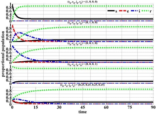
Figure 2. Proportional Populations (β = ¼ (No Epidemic)).

From the proportional population time-series, the exposed e and infected i individuals eventually decay to zero after approximately 40 days. The susceptible s and recovered r individuals reach their steady-state values in essentially the same number of days. At the end of the studied time period of 90-days, the majority of the proportional population consist of recovered r (0.9) individuals with only a small proportional population for the susceptible s (0.1) individuals.

Figure 3 demonstrates the two-dimensional phase portraits of the various combinations of the rescaled variables using the initial conditions of (s(0), e(0), i(0), r(0)) = (0.25, 0.25, 0.25, 0.25).

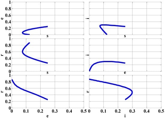
Figure 3. Phase Portraits with Initial Conditions (s(0), e(0), i(0), r(0)) = (0.25, 0.25, 0.25, 0.25) (β = ¼ (No Epidemic)).

With the assorted phase portraits, the initial conditions (s(0), e(0), i(0), r(0)) for the rescaled variables s, e, i, and r always reach the DFE equilibrium point ${\overline{X}}_{DFE}$ since it is locally stable for the case of no epidemic (β = ¼).

5.2. Epidemic

From the numerical values of the model parameters and inverse model parameters and constants with β = 4 (4 susceptible individuals who become exposed by infected individuals and leave the susceptible class and enter the exposed class per day) for the rescaled SEIRS model in (18), the epidemic condition R₀ was calculated as R₀ = 3.49840, which is greater than unity and implies epidemic for the infectious disease. Table 7 displays the DFE and EE equilibrium points ${\overline{X}}_{DFE}$ and ${\overline{X}}_{EE}$ and eigenvalues λ_i of the Jacobian matrices $J\left({\overline{X}}_{DFE}\right)$ and $J\left({\overline{X}}_{EE}\right)$ along with their local stabilities.

Table 7. Local Stability (β = 4 (Epidemic)).

Point	s	e	i	λ1	λ2	λ3	Stability
DFE	0.12501	0	0	−0.57148	−0.65737	0.18107	Unstable
EE	0.03573	0.08928	0.20825	−1.3929	−0.34731	−0.14062	Stable

In contrast to the no epidemic case (β = ¼), the epidemic case (β = 4) causes the DFE and EE equilibrium points ${\overline{X}}_{DFE}$ and ${\overline{X}}_{EE}$ to have different locally stability. With the eigenvalues λ_i of the DFE and EE equilibrium points ${\overline{X}}_{DFE}$ and ${\overline{X}}_{EE}$, the DFE equilibrium point ${\overline{X}}_{DFE}$ is locally unstable (at least one eigenvalue with non-negative real part) and the EE equilibrium point ${\overline{X}}_{EE}$ is locally stable (all eigenvalues with negative real parts) for β = 4.

Figure 4 exhibits the time-series of the proportional populations for the rescaled variables against time in days for a 90-day time period using various individual initial conditions.

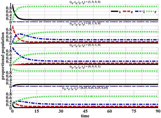
Figure 4. Proportional Populations (β = 4 (Epidemic)).

Through the proportional population time-series, the exposed e and infected i individuals do not eventually decay to zero as with the no epidemic case (β = ¼). In fact, exposed e and infected i individuals reach their steady-state of 0.0–0.2 in approximately 10–40 days. At the end of the studied time period of 90-days, the proportional population consists of recovered r (0.7–0.9) individuals and susceptible s (0.0–0.1) individuals.

Figure 5 presents the two-dimensional phase portraits of the various combinations of the rescaled variables using the initial conditions of (s(0), e(0), i(0), r(0)) = (0.25, 0.25, 0.25, 0.25).

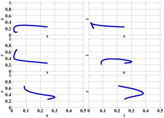
Figure 5. Phase Portraits (β = 4 (Epidemic)).

By the variety of phase portraits, the initial conditions (s(0), e(0), i(0), r(0)) for the rescaled variables s, e, i, and r always reach the EE equilibrium point ${\overline{X}}_{EE}$ since it is locally stable for the case of epidemic (β = 4).

6. Conclusions

In this paper, the author developed and implemented a new SEIRS model that capitalized on the mutual benefits of the SIR and SIRS and SEIR and SEIRS models. Fundamentally, the focus was to generalize the previous models to incorporate vital dynamics with unequal birth and death rates, vaccinations for newborns and non-newborns, and temporary immunity for communicating the advancement of infectious diseases. From the experimental results of the proposed and rescaled SEIRS model, the local stability of the DFE ${\overline{X}}_{DFE}$ and EE ${\overline{X}}_{EE}$ equilibrium points were examined for the cases of no epidemic (R₀ ≤ 1) and epidemic (R₀ > 1) using the time-series and phase portraits of the susceptible s, exposed e, infected i, and recovered r individuals. Whereas the exposed e and infected i individuals eventually decayed to zero after approximately 40 days (no epidemic), the exposed e and infected i individuals reached their steady-state of 0.0–0.2 in approximately 10–40 days (epidemic). In the no epidemic case, the proportional population consisted of recovered r (0.9) individuals with only a small proportional population for the susceptible s (0.1) individuals. For the epidemic case, the proportional population consisted primarily of the recovered r (0.7–0.9) individuals and susceptible s (0.0–0.1) individuals. For both the no epidemic and epidemic cases, the initial conditions for the susceptible s, exposed e, infected i, and recovered r individuals reached the corresponding equilibrium point for local stability: no epidemic (DFE ${\overline{X}}_{DFE}$) and epidemic (EE ${\overline{X}}_{EE}$). For future work, the SEIRS model with vital dynamics, vaccinations, and temporary immunity could be modified to incorporate age structure, infection-age structure, and spatial structure along with treatment, isolation, quarantines, and vertical transmission to obtain even more realistic epidemic mathematical models.

References

- Brauer, F.; Van den Driessche, P.; Wu, J. Mathematical Epidemiology; Springer: New York, NY, USA, 2008; p. 415. [Google Scholar]
- Ma, Z.; Li, J. Dynamic Modeling and Analysis of Epidemics; World Scientific: Singapore, Singapore, 2009; p. 513. [Google Scholar]
- Murray, J.D. Mathematical Biology I. An Introduction, 3rd ed.; Springer: New York, NY, USA, 2002; p. 576. [Google Scholar]
- Sontag, E.D. Lecture Notes on Mathematical Systems Biology; Rutgers University: New Brunswick, NJ, USA, 2014; Available online: http://www.math.rutgers.edu/~sontag/FTPDIR/systems_biology_notes.pdf (accessed on 16 January 2017).
- Kermack, W.O.; McKendrick, A.G. A Contribution to the Mathematical Theory of Epidemics. Proc. R. Soc. A 1927, 115, 700–721. [Google Scholar] [CrossRef]
- Kermack, W.O.; McKendrick, A.G. Contributions to the Mathematical Theory of Epidemics. II. The Problem of Endemicity. Proc. R. Soc. A 1932, 138, 55–83. [Google Scholar] [CrossRef]
- Hethcote, H. Qualitative Analyses of Communicable Disease Models. Math. Biosci. 1976, 28, 335–356. [Google Scholar] [CrossRef]
- Hethcote, H. The Mathematics of Infectious Diseases. Soc. Ind. Appl. Math. 2000, 42, 599–653. [Google Scholar] [CrossRef]
- Anderson, R.M.; May, R.M. Population biology of infectious diseases: Part I. Nature 1979, 280, 361–367. [Google Scholar] [CrossRef] [PubMed]
- Anderson, R.M.; May, R.M. Population biology of infectious diseases: Part II. Nature 1979, 280, 455–461. [Google Scholar] [CrossRef]
- Anderson, R.M.; May, R.M. Directly Transmitted Infectious Diseases: Control by Vaccination. Science 1982, 215, 1053–1060. [Google Scholar] [CrossRef] [PubMed]
- Anderson, R.M.; May, R.M. Vaccination and herd immunity to infectious diseases. Nature 1985, 318, 323–329. [Google Scholar] [CrossRef] [PubMed]
- D’Onofrio, A. On pulse vaccination strategy in the SIR epidemic model with vertical transmission. Appl. Math. Lett. 2005, 18, 729–732. [Google Scholar] [CrossRef]
- Buonomo, B.; d’Onofrio, A.; Lacitignola, D. Global stability of an SIR epidemic model with information dependent vaccination. Math. Biosci. 2008, 216, 9–16. [Google Scholar] [CrossRef] [PubMed]
- Li, M.Y.; Muldowney, J.S. Global Stability for the SEIR Model in Epidemiology. Math. Biosci. 1994, 28, 155–164. [Google Scholar] [CrossRef]
- D’Onofrio, A. Stability properties of pulse vaccination strategy in SEIR epidemic model. Math. Biosci. 2002, 179, 57–72. [Google Scholar] [CrossRef]
- Zhang, J.; Ma, Z. Global dynamics of an SEIR epidemic model with saturating contact rate. Math. Biosci. 2003, 30, 15–32. [Google Scholar] [CrossRef]
- Li, M.Y.; Graef, J.R.; Wang, L.; Karsai, J. Global dynamics of a SEIR model with varying total population size. Math. Biosci. 1999, 160, 191–213. [Google Scholar] [CrossRef]
- Zhang, J.; Li, J.; Ma, Z. Global Dynamics of an SEIR Epidemic Model with Immigration of Different Compartments. Acta Math. Sci. 2006, 26, 551–567. [Google Scholar] [CrossRef]
- Zhao, Z.; Chen, L.; Song, X. Impulsive vaccination of SEIR epidemic model with time delay and nonlinear incidence rate. Math. Comput. Simul. 2008, 79, 500–510. [Google Scholar] [CrossRef]
- Li, G.; Jin, Z. Global stability of a SEIR epidemic model with infectious force in latent, infected and immune period. Chaos Solitons Fractals 2005, 25, 1177–1184. [Google Scholar] [CrossRef]
- Li, G.; Wang, W.; Jin, Z. Global stability of an SEIR epidemic model with constant immigration. Chaos Solitons Fractals 2006, 30, 1013–1019. [Google Scholar] [CrossRef]
- Feng, Z. Final and Peak Epidemic Sizes for SEIR Models with Quarantine and Isolation. Math. Biosci. Eng. 2007, 4, 675–686. [Google Scholar] [CrossRef] [PubMed]
- Li, J.; Cui, N. Dynamic Analysis of an SEIR Model with Distinct Incidence for Exposed and Infectives. Sci. World J. 2013, 2013, 871393. [Google Scholar] [CrossRef] [PubMed]
- Safi, M.A.; Imran, M.; Gumel, A.B. Threshold dynamics of a non-autonomous SEIRS model with quarantine and isolation. Theory Biosci. 2012, 131, 19–30. [Google Scholar] [CrossRef] [PubMed]
- Safi, M.A.; Garba, S.M. Global Stability Analysis of SEIR Model with Holling Type II Incidence Function. Comput. Math. Methods Med. 2012, 2012, 826052. [Google Scholar] [CrossRef] [PubMed]
- Zhang, T.; Teng, Z. On a Nonautonomous SEIRS Model in Epidemiology. Bull. Math. Biol. 2007, 69, 2537–2559. [Google Scholar] [CrossRef] [PubMed]
- Rost, G.; Huang, S.Y.; Szekely, L. On a SEIR Epidemic Model with Delay. Dynam. Syst. Appl. 2012, 21, 33–48. [Google Scholar]
- Smith, H.L.; Wang, L.; Li, M.Y. Global Dynamics of an SEIR Epidemic Model with Vertical Transmission. SIAM J. Appl. Math. 2001, 62, 58–69. [Google Scholar] [CrossRef]
- Yan, P.; Liu, S. SEIR Epidemic Model with Delay. Aust. N. Z. Ind. Appl. Math. J. 2006, 48, 119–134. [Google Scholar] [CrossRef]
- Li, X.Z.; Fang, B. Stability of an Age-structured SEIR Epidemic Model with Infectivity in Latent Period. Appl. Appl. Math. 2009, 1, 218–236. [Google Scholar]
- Yi, N.; Zhang, Q.; Mao, K.; Yang, D.; Li, Q. Analysis and control of an SEIR epidemic system with nonlinear transmission rate. Math. Comput. Model. 2009, 50, 1498–1513. [Google Scholar] [CrossRef]
- Sun, C.; Hsieh, Y.H. Global analysis of an SEIR model with varying population size and vaccination. Appl. Math. Model. 2010, 34, 2685–2697. [Google Scholar] [CrossRef]
- Gao, S.; Chen, L.; Teng, Z. Impulsive Vaccination of an SEIRS Model with Time Delay and Varying Total Population Size. Bull. Math. Biol. 2007, 69, 731–745. [Google Scholar] [CrossRef] [PubMed]
© 2017 by the author. Licensee MDPI, Basel, Switzerland. This article is an open access article distributed under the terms and conditions of the Creative Commons Attribution (CC BY) license ( http://creativecommons.org/licenses/by/4.0/).