1. Introduction
A topological index is a real number derived from the structure of a graph in a way that does not depend on the labeling of the vertices. Hence, isomorphic graphs have the same values of topological indices. Chemical graph theory is a branch of mathematical chemistry that is mostly concerned with finding topological indices of chemical graphs that correlate well with certain physico-chemical properties of the corresponding molecules. The basic idea behind this approach is that the physico-chemical properties are governed by the mechanism depending mostly on the valences of atoms and on their relative positions within the molecule. Since both concepts are well described in graph-theoretical terms, there are reasons to believe that chemical graphs capture enough information about real molecules to make them useful as their models.
Hundreds of different topological indices have been investigated so far and have been employed in QSAR (Quantitative Structure Activity Relationship)/QSPR (Quantitative Structure Property Relationship) studies, with various degrees of success. Most of the more useful invariants belong to one of two broad classes: they are either distance based, or bond additive. The first class contains the indices that are defined in terms of distances between pairs of vertices; the second class contains the indices defined as the sums of contributions over all edges. Typical representants of the first type are the Wiener index and its various modifications; characteristic for the second type are the Randić index [
1] and the two Zagreb indices.
Another distance-based topological index of the graph
G is the Harary index. The Harary index of a graph
G, denoted by
, was introduced independently by Plavšić et al. [
2] and by Ivanciuc et al. [
3] in 1993. The Harary index is defined as follows:
where the summation goes over all pairs of vertices of G and
denotes the distance of the two vertices
u and
v in the graph
G. For a list of new results about the Harary index see [
4,
5,
6,
7].
The additively weighted version of the Harary index was introduced by Alizadeh et al. [
8] in 2013. For a given graph
G, its additively weighted Harary index
is defined as:
where
denotes the degree of vertex
u in
G. It is obvious that, if
G is a
k-regular graph, then
.
Also, in the paper [
8], they posed the following question:
What is the behavior of when G is a composite graph resulting for example by: splice, link, corona and rooted product?In this paper we investigate the behavior of under these four operations which are useful in chemistry. Also, we try to obtain upper and lower bounds for of these operations.
2. Preliminary Results
All graphs considered in this paper are finite, simple and connected. For a given graph G we denote by its vertex set, and by its edge set. The cardinalities of these two sets are denoted by n and e, respectively. The degree of a vertex is denoted by and the distance between vertices u and v in G is the length of any shortest path in G connecting u and v. The diameter of the graph G, denoted by , is . We denote by and the complete graph and the path graph with n vertices, respectively.
A regular graph is a graph where each vertex has the same number of neighbors. A regular graph with vertices of degree k is called a k-regular graph or regular graph of degree k.
The first and the second Zagreb indices of a graph
G are defined as follows:
These topological indices were conceived in the 1970s [
9,
10]. In 2008, in [
11] the first and the second Zagreb coindices of a graph
G are defined as follows:
Also, the first and the second Zagreb coindices of graph
G with
n vertices and
e edges are equal to
and
, respectively. For the proof of these facts, we refer the readers to [
12]. We will use Zagreb indices and Zagreb coindices to formulate our results in a more compact way.
For a graph G with , we define and . Also we define .
In the rest of the paper any sum denotes the sum , where is the contribution of pair to the sum.
In the sequel of this paper we denote by , for the number of vertices and the number of edges of G and we denote by , for the same quantities for H.
3. Main Results
In this section we introduce the standard graph products resulting in composite graphs and then we present explicit formulas for the values of additively weighted Harary indices of them.
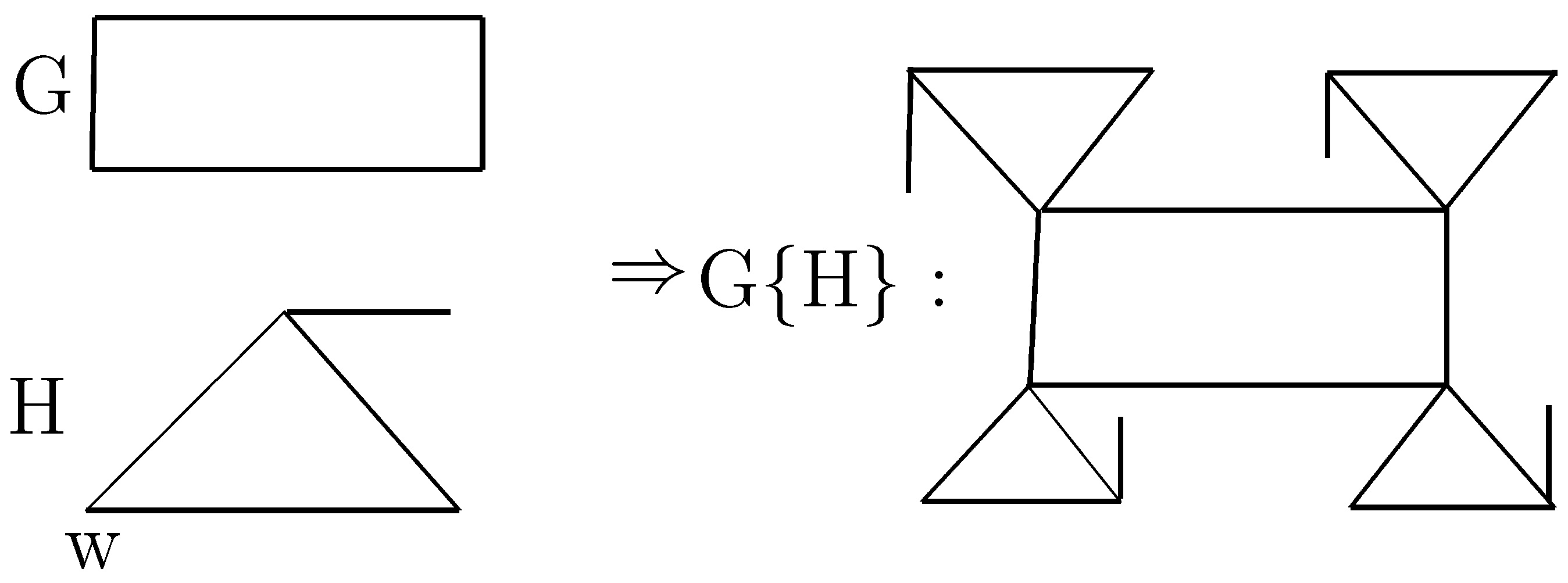
3.1. Rooted Product
Definition 1. The rooted product is obtained by taking one copy of G and copies of a rooted graph H, and by identifying the root of the i-th copy of H with the i-th vertex of G, .
For the rooted product
we have:
As an example for rooted product see
Figure 1.
Lemma 1. Let G be a simple graph and H be a rooted graph with w as its root. Then for a vertex u of such that , we have , and for a vertex v of such that we have , where is the corresponding vertex in H as v of . Also:- (1)
if , then
- (2)
if , where , then , where is the root of and is the corresponding vertex in H as v of ,
- (3)
if , where , then , where and are the corresponding vertices in H as u and v of ,
- (4)
if and , then , where is the root of and is the root of . Also, and are the corresponding vertices in H as u of and v of , respectively.
Proof. The proof is straightforward. ☐
Theorem 1. Let G be a simple graph and H be a rooted graph with w as its root. Then: Proof. From the definition we have:
By Lemma 1, we partition the sum into four sums
,
1, 2, 3, 4, where:
Thus we complete the proof of this theorem. ☐
Based on Theorem 1, we obtain the next corollary immediately.
Corollary 1. Let G be a r-regular graph and H be a k-regular rooted graph with w as its root. Then: We can determine a lower and an upper bound for , where G is a r-regular graph and H is a k-regular rooted graph.
We know that
, where
,
and
is the diameter of
G. Similarly, we have
, where
,
and
is the diameter of
H. Hence, we have:
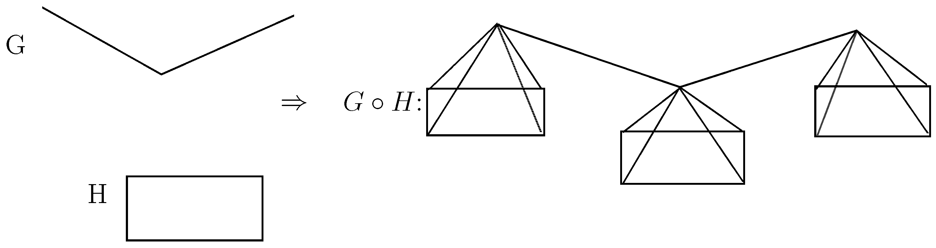
3.2. Corona
Definition 2. Let G and H be two graphs. The corona product is obtained by taking one copy of G and copies of H; and by joining each vertex of the i-th copy of H to the i-th vertex of G, 1, 2, ..., .
For the corona product
, we have:
As an example for the corona product see
Figure 2.
Lemma 2. Let G and H be two simple connected graphs. For a vertex u of such that , we have , and for a vertex v of such that , we have . Also:- (1)
if , then
- (2)
if , where , then , where is the i-th vertex in G,
- (3)
if , where , then: - (4)
if and , then , where is the i-th and is the j-th vertices in G.
Proof. The proof is obvious. ☐
Lemma 3. Let G be a simple graph and be the complete graph of order 2. Then: Proof. We partition the sum in the formula of
into three sums
such that
is over
for
1, 2, 3, where:
,
,
,
where
is the
i-th copy of
and
is the
j-th copy of
in
.
Theorem 2. Let G and H be simple graphs. Then: Proof. By Lemma 2, we partition the sum into four sums
,
. We consider four sums
as follows:
Now we consider the following relation:
Now we consider the following relation:
Note that the last equality holds in view of the fact that
. So:
Now we consider the following relation, where
By using Lemma 3 we have:
The result now follows by adding the four contributions and simplifying the expression. ☐
We note that and and the result is similar to Example 1.
Corollary 2. Let G be a r-regular graph and H be a simple graph. Then: 3.3. Splice
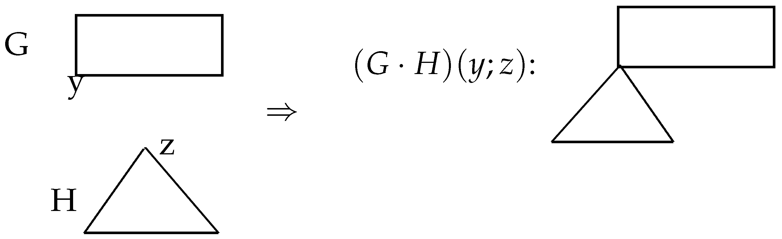
Definition 3. For given vertices and the splice of G and H by vertices y and z, which is denoted by , is defined by identifying the vertices y and z in the union of G and H.
As an example for the splice of
G and
H see
Figure 3.
Then for the splice of
G and
H by vertices
y and
z we have:
Lemma 4. Let G and H be simple graphs with disjoint vertex sets. For given vertices and suppose that the splice of G and H by vertices y and z is denoted by for convenience. Then for a vertex u of such that we have and for a vertex v of such that we have and Also:- (1)
if , then
- (2)
if , then
- (3)
if , then
Proof. The proof is obvious. ☐
Theorem 3. Let G and H be two simple graphs. For vertices and , consider . Then: Proof. For convenience we denote
by
. By definition we have:
We partition the sum into three sums such that is over for , where , ,
Similarly, we have
. Also:
The result now follows by adding the three sums , . ☐
Corollary 3. Let G be a r-regular graph and H be a k-regular graph. For vertices and , consider . Then: We can determine a lower and an upper bound for , where G and H are r-regular and k-regular graphs, respectively.
We know that
, where
and
is the diameter of
G. Similarly, we have
, where
and
is the diameter of
H. Hence, we have:
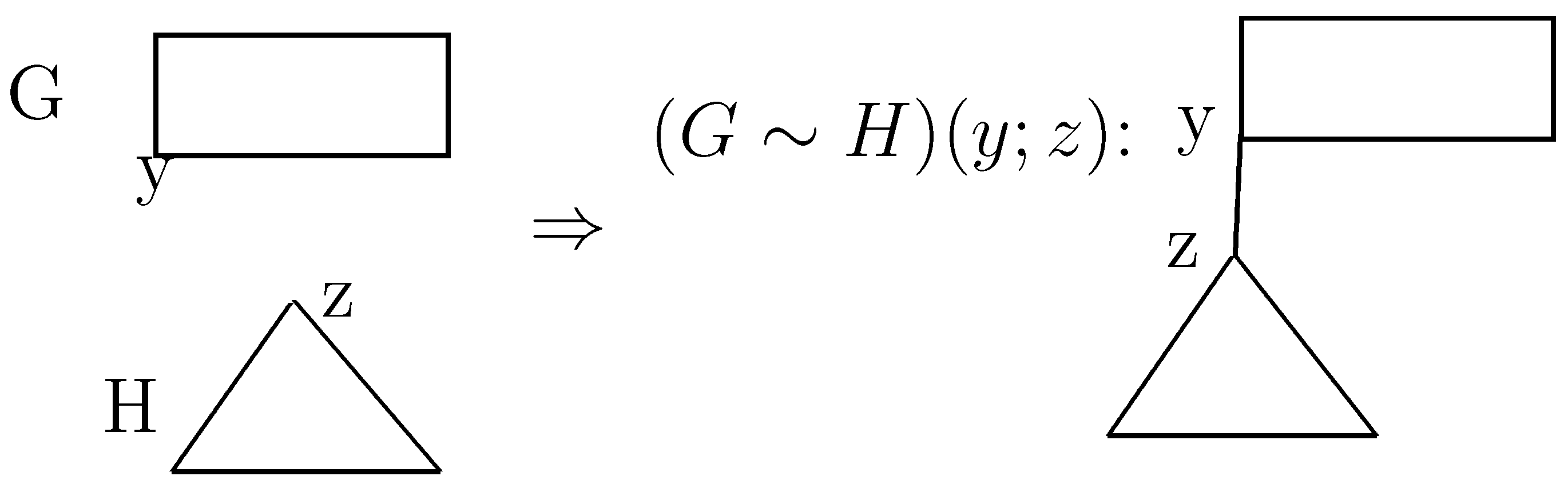
3.4. Link
Definition 4. A link of G and H by vertices y and z, which is denoted by , is defined as the graph obtained by joining y and z by an edge in the union of these graphs.
As an example of the link of two graphs see
Figure 4.
For a link of
G and
H by vertices
y and
z we have:
Lemma 5. Let G and H be two simple graphs with disjoint vertex sets. For given vertices and suppose a link of G and H by vertices y and z is denoted by for convenience. Then for a vertex u of such that we have and for a vertex v of such that we have and . Also:- (1)
if , then ,
- (2)
if , then ,
- (3)
if , then
Proof. The proof is straightforward. ☐
Theorem 4. Let G and H be two simple graphs. For vertices and , consider . Then: Proof. For convenience we denote
by
. By definition we have:
Similarly to the proof of Theorem 3, we partition the sum into three sums
such that
is over
for
, where:
,
,
We consider three sums
,
,
as follows:
Similarly, we have
. Also:
We obtain the result by adding the three sums , . ☐
Corollary 4. Let G be a r-regular graph and H be a k-regular graph. For vertices and , consider . Then: Similarly, we can determine a lower and an upper bound for , where G and H are r-regular and k-regular graphs, respectively.
We know that
, where
and
is the diameter of
G. Similarly, we have
, where
and
is the diameter of
H. So we have:
Remark 1. From the definition of and , it is obvious that the complete graph has the largest and among all graphs on the same number of vertices. So, for any graph G on n vertices we have and . Also, from the fact that adding an edge to G will increase its additively weighted Harary index, it immediately follows that the complete graph has the largest among all graph on the same number of vertices. Hence, for any graph G on n vertices we have .
From the above remark, we obtain the next corollaries immediately.
Corollary 5. Let G be a r-regular graph and H be a k-regular rooted graph. Then: Corollary 6. Let G be a r-regular graph and H be a k-regular graph. Then: 4. Conclusions
In this paper we have investigated the additively weighted Harary index for some graph products such as splice, link, corona and rooted product. Also we have determined lower and upper bounds for some of them.


