Article

Fourier Spectral Methods for Some Linear Stochastic Space-Fractional Partial Differential Equations

1
Department of Mathematics, LuLiang University, Lishi 033000, China
2
Department of Mathematics, University of Chester, Chester CH1 4BJ, UK
*
Author to whom correspondence should be addressed.
These authors contributed equally to this work.
Mathematics 2016, 4(3), 45; https://doi.org/10.3390/math4030045
Submission received: 13 March 2016 / Revised: 13 June 2016 / Accepted: 15 June 2016 / Published: 1 July 2016
(This article belongs to the Special Issue Fractional Differential and Difference Equations)

Abstract

:
Fourier spectral methods for solving some linear stochastic space-fractional partial differential equations perturbed by space-time white noises in the one-dimensional case are introduced and analysed. The space-fractional derivative is defined by using the eigenvalues and eigenfunctions of the Laplacian subject to some boundary conditions. We approximate the space-time white noise by using piecewise constant functions and obtain the approximated stochastic space-fractional partial differential equations. The approximated stochastic space-fractional partial differential equations are then solved by using Fourier spectral methods. Error estimates in the L 2 -norm are obtained, and numerical examples are given.

1. Introduction

In this paper, we will consider a Fourier spectral method for solving the following linear stochastic space fractional partial differential equation:
u ( t , x ) t + ( Δ ) α u ( t , x ) = 2 W ( t , x ) t x , 0 < t < T , 0 < x < 1
u ( t , 0 ) = u ( t , 1 ) = 0 , 0 < t < T
u ( 0 , x ) = u 0 ( x ) , 0 < x < 1
where ( Δ ) α , 1 / 2 < α 1 , is the fractional Laplacian and 2 W ( t , x ) t x is the mixed second order derivative of the Brownian sheet [1]. It is well known that the Laplacian Δ has eigenpairs ( λ j , e j ) with λ j = j 2 π 2 , e j = 2 sin j π x , j = 1 , 2 , 3 , subject to the homogeneous Dirichlet boundary conditions on ( 0 , 1 ) , i.e., e j ( 0 ) = e j ( 1 ) = 0 and:
Δ e j = λ j e j , j = 1 , 2 , 3 , .
Let H = L 2 ( 0 , 1 ) with inner product ( · , · ) and norm · . For any r R , we denote:
H 0 r : = v : v = j = 1 ( v , e j ) e j , where j = 1 λ j r ( v , e j ) 2 <
with norm:
| v | r = ( j = 1 λ j r ( v , e j ) 2 ) 1 / 2
Then, for any v H 0 2 α ( 0 , 1 ) , 1 / 2 < α 1 , we have:
( Δ ) α v = j = 1 ( v , e j ) λ j α e j
Space-fractional partial differential equations are widely used to model complex phenomena, for example quasi-geostrophic flows, fast rotating fluids, the dynamics of the frontogenesis in meteorology, diffusion in a fractal or disordered medium, pollution problems, mathematical finance and the transport problems; see, e.g., [2,3,4,5,6].
Let us here consider two examples, which apply the fractional Laplacian in the physical models. The first example is the surface quasi-geostrophic (SQG) equation,
t θ + u · θ + κ ( Δ ) α θ = 0
where κ 0 and α > 0 , θ = θ ( x 1 , x 2 , t ) denotes the potential temperature, u = ( u 1 , u 2 ) is the velocity field determined by θ . When κ > 0 , the SQG equation takes into account the dissipation generated by a fractional Laplacian. The SQG equation with κ > 0 and α = 1 / 2 arises in geophysical studies of strongly-rotating fluids. For the dissipative SQG equation, α = 1 / 2 appears to be a critical index. In the subcritical case when α > 1 / 2 , the dissipation is sufficient to control the nonlinearity, and the global regularity is a consequence of a global a priori bound. In the critical case when α = 1 / 2 , the global regularity issue is more delicate. There are few theoretical results for the supercritical case α < 1 / 2 in the literature [7].
The second example is about the wave propagation in complex solids, especially viscoelastic materials (for example, polymers) [8]. In this case, the relaxation function has the form k ( t ) = c t ν , 0 < ν < 1 , c R , instead of the exponential form known in the standard models. This polynomial relaxation is due to the non-uniformity of the material. The far field is then described by a Burgers equation with the leading operator ( Δ ) 1 + ν 2 instead of the Laplacian:
t u = ( Δ ) 1 + ν 2 u + x ( u 2 )
This equation also describes the far-field evolution of acoustic waves propagating in a gas-filled tube with a boundary layer.
Frequently, the initial value or the coefficients of the equation are random; therefore, it is natural to consider the stochastic space-fractional partial differential equations. The existence, uniqueness and regularities of the solutions of stochastic space-fractional partial differential equations have been extensively studied; see, for example, [3,4,9,10]. In this work, we will focus on the case 1 / 2 < α 1 , since the existence, uniqueness and regularity of the solution in this case is well understood in the literature; see [11] (Theorem 1.3). However, the numerical methods for solving space-fractional stochastic partial differential equations are quite restricted even for the case 1 / 2 < α 1 . Debbi and Dozzi [11] introduced a discretization of the fractional Laplacian and used it to obtain an approximation scheme for the fractional heat equation perturbed by a multiplicative cylindrical white noise. As far as we know, [11] is the only existing paper in the literature that deals with this kind of numerical approach for such a problem. In this work, we will use the ideas developed in [12] to consider the numerical methods for solving stochastic space-fractional partial differential equations; see also [13,14,15,16]. We first approximate the space-time white noise by using piecewise constant functions and then obtain the approximate solution u ^ ( t ) of the exact solution u ( t ) . Finally, we provide error estimates in the L 2 -norm for u ( t ) u ^ ( t ) .
For the deterministic space-fractional partial differential equations, many numerical methods are available in the literature. There are two ways to define the fractional Laplacian. One way of defining ( Δ ) α v ,   1 / 2 < α 1 is by using the eigenvalues and eigenfunctions of the Laplacian Δ subject to the boundary conditions as in (4). Another way of defining ( Δ ) α v ,   1 / 2 < α 1 is by using the integral for the function v ˜ , where v ˜ is defined on the whole real line R and is the extension function of v:
v ˜ ( x ) = v ( x ) , 0 < x < 1 0 , x ( 0 , 1 )
More precisely, for v ˜ ( x ) , x R , we define:
( Δ ) α v ˜ ( x ) = C α R { 0 } 2 v ˜ ( x ) + v ˜ ( x + y ) v ˜ ( x y ) | y | 1 + 2 α d y , x R
where C α is a positive constant depending on α . We then define [17],
( Δ ) α v ˜ ( x ) = F 1 | ξ | 2 α ( F ( v ˜ ) ) ( ξ ) , x R
where F and F 1 denote the Fourier and inverse Fourier transforms, respectively. For v ( x ) , x ( 0 , 1 ) , we define the fractional Laplacian by:
( Δ ) α v ( x ) = ( Δ ) α v ˜ ( x )
It is easy to show that for some suitable functions w ( x ) , x R [18],
( Δ ) α w ( x ) = F 1 | ξ | 2 α w ( ξ ) = 1 2 cos ( π α ) R D x 2 α w ( x ) + x R D 2 α w ( x )
where R D x β w ( x ) and x R D β w ( x ) , 1 < β < 2 are called Riemann–Liouville fractional derivatives defined by:
R D x β w ( x ) = 1 Γ ( 2 β ) d 2 d x 2 x ( x y ) 1 β w ( y ) d y x R D β w ( x ) = 1 Γ ( 2 β ) d 2 d x 2 x ( y x ) 1 β w ( y ) d y
Hence, for the function v ( x ) defined on the bounded interval ( 0 , 1 ) , we have:
( Δ ) α v ( x ) = 1 2 cos ( π α ) 0 R D x 2 α v ( x ) + x R D 1 2 α v ( x ) , x ( 0 , 1 )
which is also called the Riesz fractional derivative.
We note that Definitions (4) and (5) are not equivalent [17]. For the deterministic space-fractional partial differential equations where the space-fractional derivative is defined by (5), or the Riemann-Liouville space-fractional derivative, or the Caputo space-fractional derivative, many numerical methods are available, for example, finite difference methods [18,19,20,21,22,23,24,25,26,27,28,29,30], finite element methods [14,31,32,33,34,35,36,37,38,39,40] and spectral methods [41,42]. For the deterministic space-fractional partial differential equations where the space-fractional derivative is defined by (4), some numerical methods are also available, for example the matrix transfer method (MTT) [21,22,43] and the Fourier spectral method [44]. In this work, we will use Fourier spectral methods to solve the approximated stochastic space-fractional partial differential equations. The main advantage of this approach is that it gives a full diagonal representation of the fractional operator, being able to achieve spectral convergence regardless of the fractional power in the problem. Let 0 = x 0 < x 1 < x 2 < < x J = 1 be the space partition of ( 0 , 1 ) and h the space step size. Let 0 = t 0 < t 1 < t 2 < < t N = T be the time partition of ( 0 , T ) and k the time step size. To find the approximate solution of (1)–(3), we first approximate the space-time white noise 2 W ( t , x ) t x by using a piecewise constant function 2 W ^ ( t , x ) t x defined by, with n = 1 , 2 , 3 , . . . , N , j = 1 , 2 , . . . , J [12],
2 W ^ ( t , x ) t x : = η n j k h , t n 1 t t n , x j 1 x x j
where η n j N ( 0 , 1 ) is an independently and identically distributed random variable and:
η n j = 1 k h t n 1 t n x j 1 x j d W ( t , x )
Hence:
2 W ^ ( t , x ) t x = 1 k h t n 1 t n x j 1 x j d W ( t , x ) , on [ t n 1 , t n ] × [ x j 1 , x j ]
We also note that [12]:
t n 1 t n x j 1 x j d W ^ ( t , x ) = t n 1 t n x j 1 x j 2 W ^ ( t , x ) t x d x d t
The solution u ( t , x ) of (1)–(3) can then be approximated by u ^ ( t , x ) , which solves the following:
u ^ ( t , x ) t + ( Δ ) α u ^ ( t , x ) = 2 W ^ ( t , x ) t x , 0 < t < T , 0 < x < 1
u ^ ( t , 0 ) = u ^ ( t , 1 ) = 0 , 0 < t < T
u ^ ( 0 , x ) = u 0 ( x ) , 0 < x < 1
Note that 2 W ^ ( t , x ) t x is a function in L 2 ( ( 0 , T ) × ( 0 , 1 ) ) , and therefore, we can solve (8)–(10) by using any appropriate numerical method for deterministic space-fractional partial differential equations. In Theorem 2, we prove that, if 1 / 2 < α 1 , then:
E 0 T 0 1 u ( t , x ) u ^ ( t , x ) 2 d x d t C ( k 1 1 2 α + h 2 k 2 α 3 2 α )
Let us now introduce the Fourier spectral method for solving (8)–(10). Let J be a positive integer, and denote:
S J = span { e 1 , e 2 , , e J }
Define by P J : H S J the projection from H to S J ,
P J v : = j = 1 J ( v , e j ) e j
The Fourier spectral method for solving (8)–(10) is to find u ^ J ( t ) S J , such that:
u ^ J ( t , x ) t + ( Δ ) α u ^ J ( t , x ) = P J 2 W ^ ( t , x ) t x , 0 < t < T , 0 < x < 1
u ^ J ( t , 0 ) = u ^ J ( t , 1 ) = 0 , 0 < t < T
u ^ J ( 0 , x ) = P J u 0 ( x ) , 0 < x < 1
In Theorem 4, we prove that:
u ^ ( t ) u ^ J ( t ) C u 0 P J u 0 + C 1 ( J + 1 ) α 0 t f ^ ( s ) 2 d s 1 / 2 , for 1 / 2 < α 1
Combining Theorem 2 with Theorem 4, we have:
E 0 T 0 1 u ( t , x ) u ^ J ( t , x ) 2 d x d t C ( k 1 1 2 α + h 2 k 2 α 3 2 α ) + C u 0 P J u 0 2 + C 1 ( J + 1 ) 2 α k 1 1 2 α + k 1 h 1
The paper is organized as follows. In Section 2, we consider the approximation of space-time white noise. In Section 3, we consider a Fourier spectral method for deterministic space-fractional partial differential equations, and the error estimates are proven. In Section 4, we provider a numerical example.

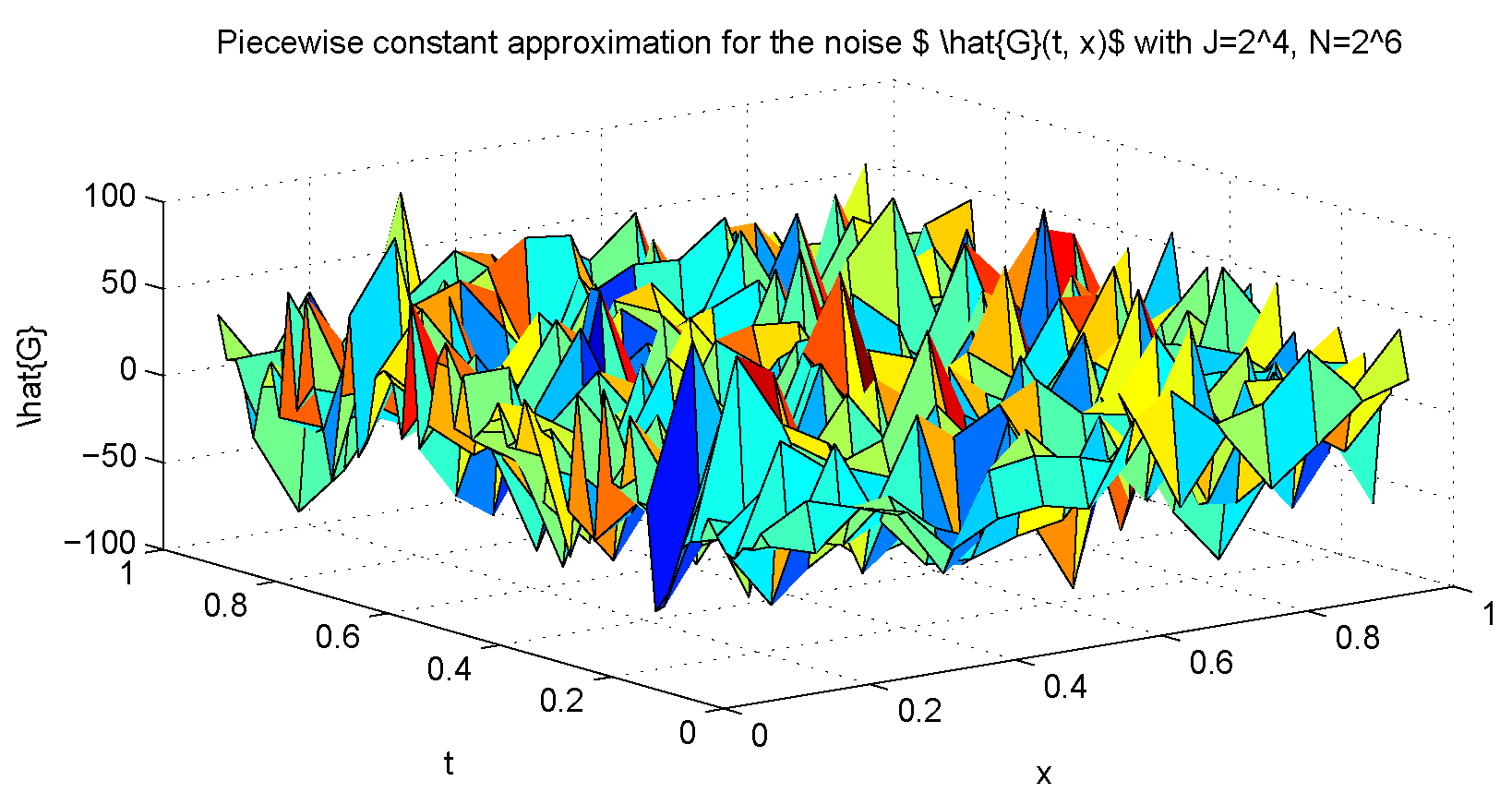
2. Approximate White Noise and Regularity

Consider the stochastic space-fractional partial differential equation:
u ( t , x ) t + ( Δ ) α u ( t , x ) = f ( t , x ) , 0 < t < T , 0 < x < 1
u ( t , 0 ) = u ( t , 1 ) = 0 , 0 < t < T
u ( 0 , x ) = u 0 ( x ) , 0 < x < 1
where f ( t , x ) = 2 W ( t , x ) t x denotes the mixed second order derivative of the Brownian sheet [12]. There is no strong solution of (17)–(19) since f ( t , x ) = 2 W ( t , x ) t x L 2 ( ( 0 , T ) × ( 0 , 1 ) ) .
The mild solution of (17)–(19) has the following form, for example [9,10],
u ( t , x ) = 0 1 G α ( t , x , y ) u 0 ( y ) d y + 0 t 0 1 G α ( t s , x , y ) d W ( s , y )
where:
G α ( t , x , y ) = j = 1 e λ j α t e j ( x ) e j ( y )
and the stochastic integral 0 t 0 1 G α ( t s , x , y ) d W ( s , y ) is well defined.
We have the following existence and uniqueness theorem, for example [9,10,11],
Theorem 1. 
[11] [Theorem 1.3] Let 1 / 2 < α 1 and β > 0 . Let u 0 be a H 0 β ( 0 , 1 ) -valued F 0 -measurable function, such that:
E u 0 H 0 β ( 0 , 1 ) p <
for some p > 4 α 2 α 1 . Then, (17)–(19) has a unique mild solution u, such that, for any 0 θ < min { 2 α 1 2 2 α p , β } ,
E sup 0 t T u ( t ) H 0 θ ( 0 , 1 ) p <
Our strategy is to approximate the solution u ( t , x ) of (17)–(19) by u ^ ( t , x ) , which satisfies the following problem:
u ^ ( t , x ) t + ( Δ ) α u ^ ( t , x ) = f ^ ( t , x ) , 0 < t < T , 0 < x < 1
u ^ ( t , 0 ) = u ^ ( t , 1 ) = 0 , 0 < t < T
u ^ ( 0 , x ) = u 0 ( x ) , 0 < x < 1
Here, f ^ ( t , x ) = 2 W ^ ( t , x ) t x is defined by (6). The solution of (21)–(23) has the form of; see, e.g., [12]:
u ^ ( t , x ) = 0 1 G α ( t , x , y ) u 0 ( y ) d y + 0 t 0 1 G α ( t s , x , y ) d W ^ ( s , y )
Theorem 2. 
Let u and u ^ be the solutions of (17)–(19) and (21)–(23), respectively. Assume that u 0 H and 1 / 2 < α 1 , then:
E 0 T 0 1 u ( t , x ) u ^ ( t , x ) 2 d x d t C ( k 1 1 2 α + h 2 k 2 α 3 2 α )
Proof. 
See the Appendix. ☐
Remark 1. 
When α = 1 , we obtain the same estimates as in [12,14], i.e.,
E 0 T 0 1 u ( t , x ) u ^ ( t , x ) 2 d x d t C ( k 1 2 + h 2 k 1 2 )
Theorem 3. 
Let u ^ be the solution of (21)–(23), then:
E t j t j + 1 0 1 u ^ t 2 ( t , x ) d x d t C ( k 1 2 α + h 1 ) , j 0
and:
E 0 1 | ( Δ ) α u ^ ( t , x ) | 2 d x C ( k 1 1 2 α + k 1 h 1 )
for any 1 / 2 < α 1 .
Proof. 
We only prove (26). The proof of (27) is similar. Note that:
u ^ ( t , x ) = 0 1 G α ( t , x , y ) u 0 ( y ) d y + 0 t 0 1 G α ( t s , x , y ) d W ^ ( s , y ) = 0 1 G α ( t , x , y ) u 0 ( y ) d y + 0 t 0 1 G α ( t s , x , y ) 2 W ^ ( s , y ) s y d y d s
and:
u ^ t ( t , x ) = 0 1 t G α ( t , x , y ) u 0 ( y ) d y + 0 t 0 1 t G α ( t s , x , y ) 2 W ^ ( s , y ) s y d y d s + 0 1 G α ( 0 , x , y ) 2 W ^ ( t , y ) t y d y
Since w ( t , x ) = 0 1 G α ( t , x , y ) w 0 ( y ) d y is the solution of the following equation:
w ( t , x ) t + ( Δ ) α w ( t , x ) = 0 , 0 < x < 1 , 0 < t < T w ( t , 0 ) = w ( t , 1 ) = 0 , 0 < t < T w ( 0 , x ) = w 0 ( x )
we therefore have:
w 0 ( x ) = 0 1 G α ( 0 , x , y ) w 0 ( y ) d y
Choose w 0 ( y ) = 2 W ^ ( t , y ) t y for fixed t; then, we have:
0 1 G α ( 0 , x , y ) 2 W ^ ( t , y ) t y d y = 2 W ^ ( t , x ) t x
Hence, by (28),
u ^ t ( t , x ) = 0 1 t G α ( t , x , y ) u 0 ( y ) d y + 0 t 0 1 t G α ( t s , x , y ) d W ^ ( s , y ) + 2 W ^ ( t , x ) t x
Using the inequality ( a + b + c ) 2 3 ( a 2 + b 2 + c 2 ) , a , b , c R , we have:
E t j t j + 1 0 1 u ^ t 2 ( t , x ) d x d t 3 E t j t j + 1 0 1 0 t 0 1 t G α ( t s , x , y ) d W ^ ( s , y ) 2 d x d t + 3 E t j t j + 1 0 1 W ^ ( t , x ) t x 2 d x d t + 3 E t j t j + 1 0 1 0 1 t G α ( t , x , y ) u 0 ( y ) d y 2 d x d t = 3 ( I + I I + I I I )
Now, I, by using ( a + b ) 2 2 ( a 2 + b 2 ) , a , b R , is written as:
I 2 E t j t j + 1 0 1 0 t j 1 0 1 t G α ( t s , x , y ) d W ^ ( s , y ) 2 d x d t + 2 E t j t j + 1 0 1 t j 1 t 0 1 t G α ( t s , x , y ) d W ^ ( s , y ) 2 d x d t = 2 ( I 1 + I 2 )
Furthermore I 1 , with η k l = N ( 0 , 1 ) , k = 0 , 1 , 2 , , J 1 , l = 0 , 1 , 2 , , j 2 , j 2 , is expressed as:
I 1 = E t j t j + 1 0 1 0 t j 1 0 1 t G α ( t s , x , y ) d W ^ ( s , y ) 2 d x d t = E t j t j + 1 0 1 1 k h l = 0 j 2 t l t l + 1 k = 0 J 1 x k x k + 1 t G α ( t s , x , y ) η k l d y d s 2 d x d t = E t j t j + 1 0 1 1 k h l = 0 j 2 k = 0 J 1 t l t l + 1 x k x k + 1 t G α ( t s , x , y ) d y d s η k l 2 d x d t = t j t j + 1 0 1 1 k h l = 0 j 2 k = 0 J 1 t l t l + 1 x k x k + 1 t G α ( t s , x , y ) d y d s 2 d x d t = t j t j + 1 0 1 1 k h l = 0 j 2 k = 0 J 1 t l t l + 1 x k x k + 1 n = 1 λ n α e λ n α ( t s ) e n ( x ) e n ( y ) d y d s 2 d x d t = C t j t j + 1 0 1 1 k h l = 0 j 2 k = 0 J 1 ( n = 1 λ n α cos n π x k + 1 cos n π x k n π e n ( x ) e λ n α ( t t l + 1 ) e λ n α ( t t l ) λ n α ) 2 d x d t
Note that ( e n , e m ) = δ n m , n , m = 1 , 2 , ; we have:
I 1 = C t j t j + 1 1 k h l = 0 j 2 k = 0 J 1 n = 1 cos n π x k + 1 cos n π x k n π 2 e λ n α ( t t l + 1 ) e λ n α ( t t l ) 1 2 d t = C t j t j + 1 1 k h l = 0 j 2 k = 0 J 1 n = 1 cos n π x k + 1 cos n π x k n π 2 e 2 λ n α ( t t l + 1 ) 1 e λ n α ( t l + 1 t l ) 2 d t = C 1 k h l = 0 j 2 k = 0 J 1 n = 1 cos n π x k + 1 cos n π x k n π 2 e 2 λ n α ( t j t l + 1 ) e 2 λ n α ( t j + 1 t l + 1 ) λ n α 1 e λ n α ( t l + 1 t l ) 2 = C 1 k h k = 0 J 1 n = 1 cos n π x k + 1 cos n π x k n π 2 ( 1 e λ n α k ) 2 λ n α l = 0 j 2 e 2 λ n α ( t j t l + 1 ) = C 1 k h n = 1 ( 1 e λ n α k ) 2 λ n α + 1 k = 0 J 1 ( cos n π x k + 1 cos n π x k ) 2 l = 0 j 2 e 2 λ n α ( t j t l + 1 )
Note that, since | cos ( n π x k + 1 ) cos ( n π x k ) | ( n π h ) 2 , then:
k = 0 J 1 ( cos n π x k + 1 cos n π x k ) 2 C k = 0 J 1 ( n π h ) 2 = C λ n h
We have, by (68) and (67):
I 1 = C 1 k h n = 1 ( 1 e λ n α k ) 2 λ n α + 1 ( λ n h ) l = 0 j 2 e 2 λ n α ( t j t l + 1 ) = C 1 k h n = 1 ( 1 e λ n α k ) 2 λ n α + 1 ( λ n h ) ( k 1 λ n α ) = C k 2 n = 1 ( 1 e λ n α k ) 2 λ n 2 α C k 2 k 4 α 1 2 α = C k 1 2 α
We remark that I 1 can also be estimated by using the following alternative way.
I 1 = E t j t j + 1 0 1 0 t j 1 0 1 t G α ( t s , x , y ) d W ^ ( s , y ) 2 d x d t = t j t j + 1 0 1 0 t j 1 0 1 t G α ( t s , x , y ) 2 d y d s d x d t = t j t j + 1 0 1 0 t j 1 0 1 n = 1 λ n α e λ n α ( t s ) e n ( x ) e n ( y ) 2 d y d s d x d t = t j t j + 1 0 t j 1 n = 1 λ n 2 α e 2 λ n α ( t s ) d s d t = t j t j + 1 n = 1 λ n 2 α e 2 λ n α ( t t j 1 ) e 2 λ n α t 2 λ n α d t
Note that t t j , we then have, by using (63),
I 1 C t j t j + 1 n = 1 λ n α e 2 λ n α k d t = C k n = 1 λ n α e 2 λ n α k C k 1 2 α
For I 2 , we have:
I 2 2 E t j t j + 1 0 1 t j 1 t j 0 1 t G α ( t s , x , y ) d W ^ ( s , y ) 2 d x d t + 2 E t j t j + 1 0 1 t j t 0 1 t G α ( t s , x , y ) d W ^ ( s , y ) 2 d x d t = 2 I 21 + 2 I 22
where I 21 can be estimated as follows:
I 21 = E t j t j + 1 0 1 1 k h k = 0 J 1 t j 1 t j x k x k + 1 t G α ( t s , x , y ) η k j d y d s 2 d x d t = t j t j + 1 0 1 1 k h k = 0 J 1 t j 1 t j x k x k + 1 t G α ( t s , x , y ) d y d s 2 d x d t = t j t j + 1 0 1 1 k h k = 0 J 1 t j 1 t j x k x k + 1 n = 1 λ n α e λ n α ( t s ) e n ( x ) e n ( y ) d y d s 2 d x d t = t j t j + 1 0 1 1 k h k = 0 J 1 [ n = 1 λ n α e λ n α ( t t j ) e λ n α ( t t j 1 ) λ n α e n ( x ) cos n π x k + 1 cos n π x k n π ] 2 d x d t = t j t j + 1 1 k h k = 0 J 1 n = 1 cos n π x k + 1 cos n π x k n π 2 e 2 λ n α ( t t j ) 1 e λ n α k 2 d t = 1 k h k = 0 J 1 n = 1 cos n π x k + 1 cos n π x k n π 2 e 2 λ n α ( t j t j ) e 2 λ n α ( t j + 1 t j ) λ n α 1 e λ n α k 2 = 1 k h n = 1 ( 1 e λ n α k ) 2 λ n α + 1 k = 0 J 1 ( cos n π x k + 1 cos n π x k ) 2 · 1 1 k h n = 1 ( 1 e λ n α k ) 2 λ n α + 1 λ n h = 1 k n = 1 ( 1 e λ n α k ) 2 λ n α 1 k n = 1 ( 1 e λ n α k ) λ n α
which implies, by (64):
I 21 1 k k 1 1 2 α = k 1 2 α
For I 22 , we have:
I 22 = E t j t j + 1 0 1 t j t 0 1 t G α ( t s , x , y ) d W ^ ( s , y ) 2 d x d t = t j t j + 1 0 1 1 k h k = 0 J 1 t j t x k x k + 1 n = 1 λ n α e λ n α ( t s ) e n ( x ) e n ( y ) d y d s 2 d x d t = t j t j + 1 0 1 1 k h k = 0 J 1 [ n = 1 λ n α e λ n α ( t t ) e λ n α ( t t j ) λ n α e n ( x ) cos n π x k + 1 cos n π x k n π d y d s ] 2 d x d t = t j t j + 1 1 k h k = 0 J 1 n = 1 cos n π x k + 1 cos n π x k n π 2 1 e λ n α k 2 d t = k 1 k h k = 0 J 1 n = 1 cos n π x k + 1 cos n π x k 2 ( 1 e λ n α k ) 2 λ n
Moreover, applying (66) and taking into account | cos ( n π x k + 1 ) cos n π x k | n π h , we derive:
I 22 1 h k = 0 J 1 n 2 π 2 h 2 n = 1 ( 1 e λ n α k ) 2 λ n n = 1 ( 1 e λ n α k ) 2 C k 1 2 α
For I I we have, with η k j = N ( 0 , 1 ) ,
I I = E t j t j + 1 0 1 W ^ ( t , x ) t x 2 d x d t = E t j t j + 1 k = 0 J 1 x k x k + 1 1 k h η k j 2 d x d t = 1 k h t j t j + 1 k = 0 J 1 x k x k + 1 d x d t = 1 k h k = h 1
Similarly, we can estimate I I I . Together, these estimates complete the proof of Theorem 3. ☐

3. Fourier Spectral Method

In this section, we will consider a Fourier spectral method for solving the deterministic space-fractional partial differential equation:
u ^ ( t , x ) t + ( Δ ) α u ^ ( t , x ) = f ^ ( t , x ) , 0 < t < T , 0 < x < 1
u ^ ( t , 0 ) = u ^ ( t , 1 ) = 0 , 0 < t < T
u ^ ( 0 , x ) = u 0 ( x ) , 0 < x < 1
where f ^ ( t , x ) = 2 W ^ ( t , x ) t x is defined by (6) and f ^ L 2 ( ( 0 , T ) × ( 0 , 1 ) ) .
Denote A = Δ with D ( A ) = H 0 1 ( 0 , 1 ) H 2 ( 0 , 1 ) . For any s > 0 and v H 0 2 s ( 0 , 1 ) , we have A s v = j = 1 λ j s ( v , e j ) e j . It is obvious that:
| v | r = A r / 2 v = j = 1 λ j r ( v , e j ) 2 1 / 2 , v H 0 r ( 0 , 1 ) , r > 0
Further, we denote E α ( t ) = e t A α , 1 / 2 < α 1 . Then, the solution of (30)–(32) can be written as the following operator form:
u ^ ( t ) = E α ( t ) u ^ 0 + 0 t E α ( t s ) f ^ ( s ) d s , u ^ J ( 0 ) = u 0
The spectral method of (30)–(32) consists of finding u ^ J ( t ) S J , such that:
u ^ J ( t , x ) t + ( Δ ) α u ^ J ( t , x ) = P J 2 W ^ ( t , x ) t x , 0 < t < T , 0 < x < 1
u ^ J ( t , 0 ) = u ^ J ( t , 1 ) = 0 , 0 < t < T
u ^ J ( 0 , x ) = P J u 0 ( x ) , 0 < x < 1
where P J : H S J is defined by (12).
Similarly, the solution of (34)–(36) has the form of:
u ^ J ( t ) = E α ( t ) P J u ^ 0 + 0 t E α ( t s ) P J f ^ ( s ) d s , u ^ J ( 0 ) = P J u 0
Theorem 4. 
Assume that u ^ and u ^ J are the solutions of (33) and (37), respectively. Let 0 r < 1 / 2 , and assume that u 0 H 0 r ( 0 , 1 ) . Then, there exists a positive constant C, such that:
| u ^ ( t ) u ^ J ( t ) | r C | u 0 P J u 0 | r + C 1 ( J + 1 ) α ( 1 r / α ) 0 t f ^ ( s ) 2 d s 1 / 2
In particular, we have, with r = 0 ,
u ^ ( t ) u ^ J ( t ) C u 0 P J u 0 + C 1 ( J + 1 ) α 0 t f ^ ( s ) 2 d s 1 / 2
To prove Theorem 4, we need the following smoothing property for the solution operator E α ( t ) .
Lemma 5. 
1.
Let s > 0 . We have:
A s E α ( t ) C t s α e δ t , t > 0 , w i t h 1 / 2 < α 1
for some constants C and δ which depend on s and α .
2.
Let P J : H S J be defined by (12), then:
E α ( t ) ( I P J ) e t λ J + 1 α v , t > 0 , w i t h 1 / 2 < α 1
Proof. 
Note that A is a positive definite operator with eigenvalues 0 < λ 1 < λ 2 < λ 3 < . For any function g ( · ) , we have:
g ( A ) = sup λ > λ 1 > 0 | g ( λ ) |
Hence, with δ = 1 2 λ 1 α ,
A s E α ( t ) = A s E α ( t / 2 ) E α ( t / 2 ) A s E α ( t / 2 ) E α ( t / 2 ) = sup λ > λ 1 λ s e t 2 λ α · sup λ > λ 1 e t 2 λ α = sup λ > λ 1 t 2 λ α s / α e t 2 λ α t 2 s / α e t 2 λ 1 α C ( t / 2 ) s / α e δ t C t s / α e δ t
which is (40). To show (41), we note that:
E α ( t ) ( I P J ) v = j = J + 1 e 2 t λ j α ( v , e j ) 2 1 / 2 e t λ N + 1 α v
The proof of Lemma 5 is complete. ☐
Proof of Theorem 4. 
Subtracting (37) from (33), we get:
u ^ ( t ) u ^ J ( t ) = E α ( t ) ( u 0 P J u 0 ) + 0 t E α ( t s ) f ( s ) P J f ( s ) d s = I + I I
For I, we have, with 0 r < 1 / 2 ,
| I | r = | E α ( t ) ( u 0 P J u 0 ) | r = A r 2 E α ( t ) u 0 P J u 0 = j = J + 1 e 2 t λ j α λ j r ( u 0 , e j ) 2 1 / 2 e t λ J + 1 α | u 0 P J u 0 | r
For I I , by virtue of Lemma 5, for some γ ( 0 , 1 ) , we get:
| I I | r = | 0 t E α ( t s ) f ^ ( s ) P J f ^ ( s ) d s | r = 0 t A r 2 E α ( t s ) I P J f ^ ( s ) d s 0 t A r 2 E α ( 1 γ ) ( t s ) E ( γ ( t s ) ) ( I P J ) f ^ ( s ) d s C 0 t ( t s ) r 2 α e κ α ( t s ) f ^ ( s ) d s
where κ α = δ ( 1 γ ) + λ J + 1 α γ .
By the Cauchy-Schwarz inequality:
| I I | r 0 ( ( t s ) r 2 α e κ ( t s ) ) 2 d s 1 / 2 · 0 t f ^ ( s ) 2 d s 1 / 2
Note that r < α and λ J + 1 = ( J + 1 ) 2 π imply:
0 e 2 κ α s s r / α d s 0 s r / α e 2 s d s κ α 1 r / α C 1 κ α 1 r / α C 1 ( λ J + 1 α ) 1 r / α C 1 ( J + 1 ) 2 α ( 1 r / α )
Thus:
| I I | r C 1 ( J + 1 ) 2 α ( 1 r / α ) 0 t f ^ ( s ) 2 d s 1 / 2
Together, these estimates complete the proof of Theorem 4. ☐
Combining Theorem 2 with Theorem 4, we obtain:
Theorem 6. 
Let u and u ^ J be the solutions of (17)–(19) and (34)–(36), respectively. Assume that u 0 H . We have:
E 0 T 0 1 u ( t , x ) u ^ J ( t , x ) 2 d x d t C ( k 1 1 2 α + h 2 k 2 α 3 2 α ) + C u 0 P J u 0 2 + C 1 ( J + 1 ) 2 α ( k 1 1 2 α + k 1 h 1 ) , f o r 1 / 2 < α 1
Proof. 
Note that:
E 0 T 0 1 u ( t , x ) u ^ J ( t , x ) 2 d x d t 2 E 0 T 0 1 u ( t , x ) u ^ ( t , x ) 2 d x d t + 2 E 0 T 0 1 u ^ ( t , x ) u ^ J ( t , x ) 2 d x d t = 2 I + 2 I I
For I, due to Theorem 2, we derive:
I C ( k 1 1 2 α + h 2 k 2 α 3 2 α )
For I I , we have:
I I = E 0 T u ^ ( t ) u ^ J ( t ) 2 d t C u 0 P J u 0 2 + C 1 ( J + 1 ) 2 α E 0 T 0 t f ^ ( s ) 2 d s d t
Note that f ^ ( s ) = u ^ s ( s ) ( Δ ) α u ^ ( s ) , and hence, by virtue of Theorem 3, we take:
E 0 T 0 t f ^ ( s ) 2 d s d t E 0 T 0 t u ^ s ( s ) ( Δ ) α u ^ ( s ) 2 d s d t C E 0 T 0 T 0 1 u ^ s 2 ( s , x ) + | ( Δ ) α u ^ ( s , x ) | 2 d x d s d t C j = 0 N k 1 2 α + h 1 C k 1 1 2 α + k 1 h 1
Together, these estimates complete the proof of Theorem 6. ☐

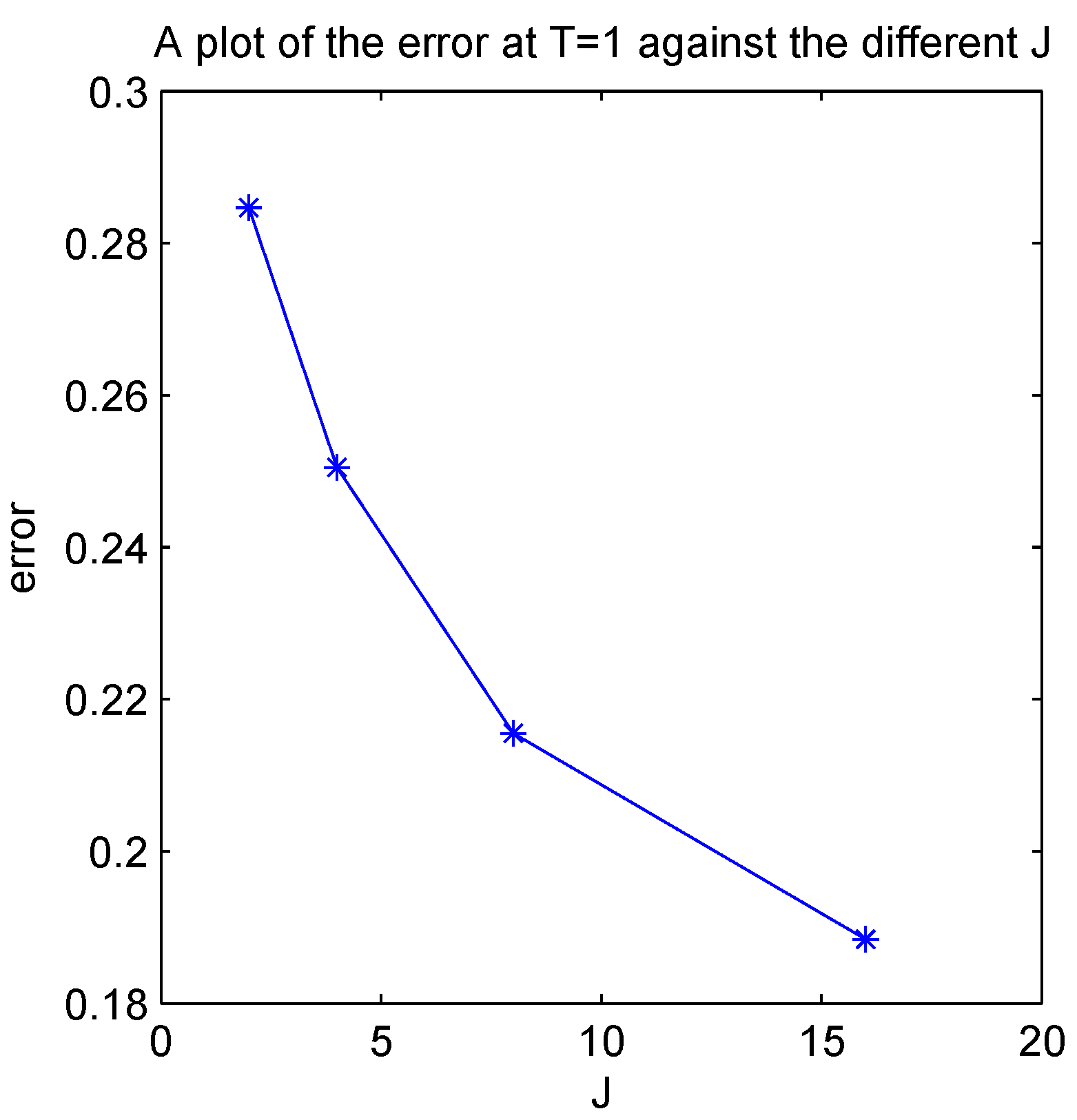
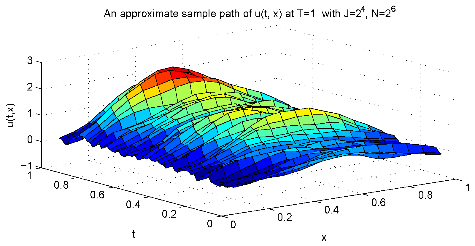
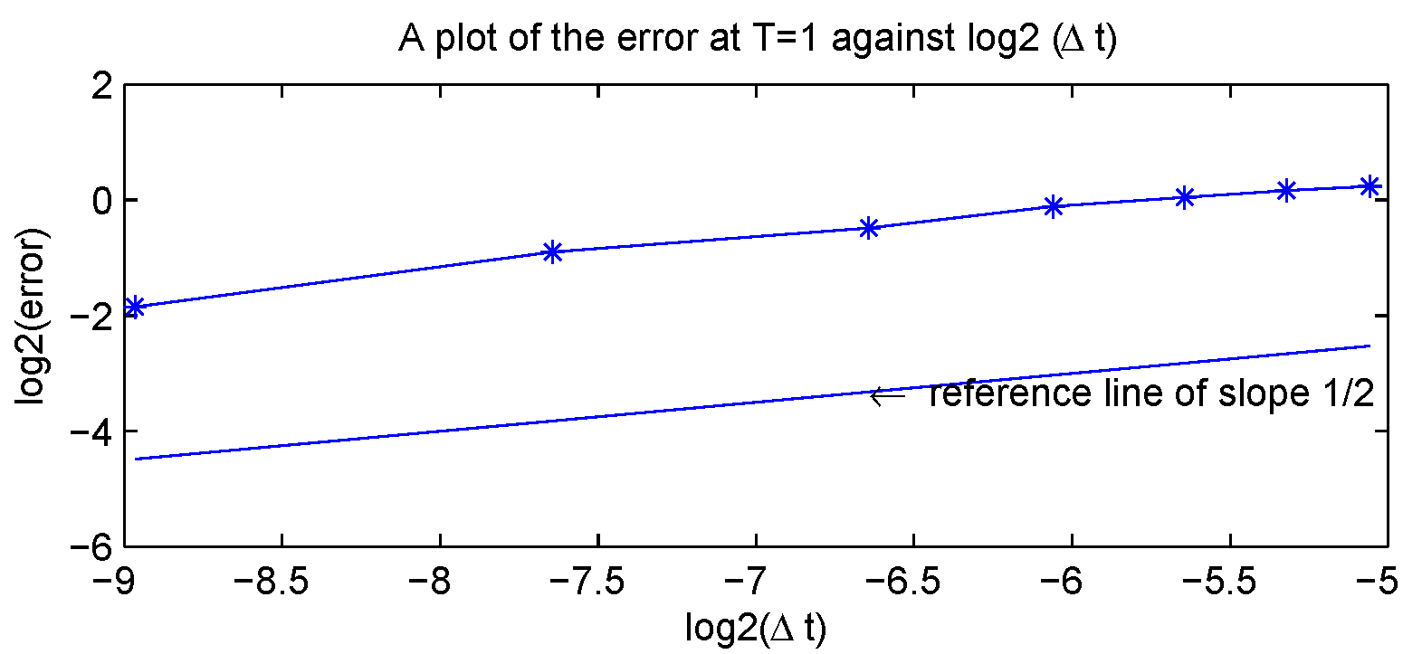
4. Numerical Simulations

In this section, we will present the computational issues for solving the following stochastic space-fractional parabolic partial differential equations by using the spectral method developed in the previous section, with 1 / 2 < α 1 ,
u ( t , x ) t + ϵ ( Δ ) α u ( t , x ) = f ( u ( t , x ) ) + 2 W ( t , x ) t x , 0 < x < 1 , 0 < t T
u ( t , 0 ) = u ( t , 1 ) = 0 , 0 < t T
u ( 0 , x ) = u 0 ( x ) , 0 < x < 1
where ( Δ ) α is the fractional Laplacian defined by using the eigenvalues and eigenfunctions of the Laplacian operator Δ subject to some boundary conditions. Here, f : R R is a smooth function, and ϵ > 0 denotes the diffusion coefficient. In our numerical example, we will use the discrete sine transform MATLAB functions dst and idst. We also include the nonlinear term f, although the error estimates in the previous sections are only proven for f = 0 . In our future work, we will consider the error estimates for solving the nonlinear stochastic space-fractional partial differential equations with multiplicative noise by using the spectral method.
Let x 0 < x 1 < < x J = 1 be a space partition of [ 0 , 1 ] and Δ x = h be the space step size. Let 0 = t 0 < t 1 < < t N = T be the time partition of [ 0 , T ] and Δ t = k the time step size. The space-time noise 2 W ( t , x ) t x is approximated by using piecewise constant function 2 W ^ ( t , x ) t x , where:
2 W ^ ( t , x ) t x = η n , j Δ t Δ x , t n 1 t t n , x j 1 x x j
For convenience, we will denote G ^ ( t , x ) = 2 W ^ ( t , x ) t x below.
Equations (43)–(45) can then be approximated by the following, with 1 / 2 < α 1 ,
u ^ ( t , x ) t + ϵ ( Δ ) α u ^ ( t , x ) = f ( u ^ ( t , x ) ) + G ^ ( t , x ) , 0 < x < 1 , 0 < t T
u ^ ( t , 0 ) = u ^ ( t , 1 ) = 0 , 0 < t T
u ^ ( 0 , x ) = u 0 ( x ) , 0 < x < 1
Denote A = 2 x 2 with D ( A ) = H 0 1 ( 0 , 1 ) H 2 ( 0 , 1 ) . Then, A has eigenvalues λ j and eigenfunctions e j where:
λ j = j 2 π 2 , e j = sin ( j π x ) , j Z +
That is:
A e j = λ j e j , j Z +
Equations (47)–(49) can further be written as the following abstract form: find u ^ ( t ) H 0 1 ( 0 , 1 ) H 2 ( 0 , 1 ) , such that:
d u ^ ( t ) d t + A u ^ ( t ) = f ( u ^ ( t ) ) + G ^ ( t ) , 0 < t T
u ^ ( 0 ) = u 0
Let S J 1 : = span { e 1 , e 2 , , e J 1 } . The spectral method for solving (47)–(49) is to find u J 1 ( t ) S J 1 , such that, with 0 < t T ,
d u ^ J 1 ( t ) d t + A J 1 u ^ J 1 ( t ) = P J 1 f ( u J 1 ( t ) ) + P J 1 G ^ ( t )
u ^ J 1 ( 0 ) = P J 1 u 0
where P J 1 : H S J 1 is the orthogonal projection operator defined by:
P J 1 v = j = 1 J 1 v ˜ j e j , v ˜ j = ( v , e j )
where A J 1 = P J 1 A : S J 1 S J 1 and ( · , · ) denotes the inner product in H = L 2 ( 0 , 1 ) . We remark that we use S J 1 (not S J ), since we will apply the MATLAB functions dst and idst in our numerical algorithms below.
The semi-implicit Euler method for solving (47)–(49) is to find u J 1 , n u J 1 ( t n ) , such that:
u ^ J 1 , n + 1 u ^ J 1 , n Δ t + A J 1 u ^ J 1 , n + 1 = P J 1 f ( u ^ J 1 , n ) + P J 1 G ^ ( t n )
u ^ J 1 , 0 = P J 1 u 0
Let:
u ^ J 1 , n = j = 1 J 1 u ˜ j , n e j S J 1
It is easy to see that the Fourier coefficients u ˜ j , n satisfy, with j = 1 , 2 , , J 1 ,
u ˜ j , n + 1 = ( 1 + Δ t λ j ) 1 u ˜ j , n + Δ t f ˜ j ( u ^ J 1 , n ) + Δ t G ˜ j , n
u ˜ j , 0 = ( P J 1 u 0 , e j )
where:
P J 1 G ^ ( t n ) = j = 1 J 1 G ˜ j , n e j S J 1 , P J 1 f ( u ^ J , n ) = j = 1 J 1 f ˜ j ( u ^ J , n ) e j
Here, u ˜ j , n , G ˜ j , n , f ˜ j ( u ^ J , n ) denote the Fourier coefficients of u ^ J 1 , n , G ^ ( t n ) and f ( u ^ J 1 , n ) , respectively.
We may use the following steps to describe how to solve (47)–(49) numerically by using the spectral method:
Step 1: Given initial value u ^ 0 ( x ) and f, we get the approximation u J 1 , 0 ( x ) = P J 1 u 0 u 0 and P J 1 f ( u ^ J 1 , 0 ) f ( u ^ 0 ( x ) ) .
Step 2: Find the Fourier coefficients u ˜ j , 0 and f ˜ j ( u ^ J 1 , 0 ) by:
u ˜ 1 , 0 u ^ 2 , 0 u ^ J 1 , 0 = ( 2 ) 1 J 2 1 · dst u 0 ( x 1 ) u 0 ( x 2 ) u 0 ( x J )
f ˜ 0 ( u J , 0 ) f ˜ 1 ( u J , 0 ) f ˜ J ( u J , 0 ) = ( 2 ) 1 J 2 1 · dst f ( u 0 ( x 1 ) ) f ( u 0 ( x 2 ) ) f ( u 0 ( x J ) )
and:
G ˜ 0 , 0 G ˜ 1 , 0 G ˜ J 1 , 0 = ( 2 ) 1 J 2 1 · dst G ^ ( t 0 , x 1 ) G ^ ( t 0 , x 2 ) G ^ ( t 0 , x J 1 )
Here, G ^ ( t 0 , x 1 ) G ^ ( t 0 , x 2 ) G ^ ( t 0 , x J 1 ) = W ^ ( 1 , : ) , and W ^ is generated by:
W ^ = 1 Δ t Δ x * randn ( N , J 1 )
Step 3: Find the Fourier coefficients u ˜ j , 1 , j = 1 , 2 , , J by:
u ˜ 1 , 1 u ˜ 2 , 1 u ^ J 1 , 1 = G G . / E E
where . / denotes the element-wise division and:
G G = ( 2 ) 1 J 2 1 · dst u 0 ( x 1 ) u 0 ( x 2 ) u 0 ( x J ) + Δ t ( 2 ) 1 J 2 1 · dst f ( u 0 ( x 1 ) ) f ( u 0 ( x 2 ) ) f ( u 0 ( x J ) ) + Δ t ( 2 ) 1 J 2 1 · dst G ^ ( t 0 , x 1 ) G ^ ( t 0 , x 2 ) G ^ ( t 0 , x J 1 )
with λ j = π j ,
E E = 1 + Δ t * λ 1 2 1 + Δ t * λ 2 2 1 + Δ t * λ J 1 2
Step 4: Find the Fourier coefficients u ˜ j , 2 , j = 1 , 2 , , J 1 by:
u ^ j , 2 = ( 1 + Δ t λ j ) 1 u ˜ j , 1 + Δ t f ˜ j ( u ^ J 1 , 1 ) + Δ t G ˜ j , 1
where:
f ˜ 1 ( u ^ J 1 , 1 ) f ˜ 2 ( u ^ J 1 , 1 ) f ˜ J 1 ( u ^ J 1 , 1 ) = ( 2 ) 1 J 2 1 · dst f ( u ^ J 1 , 1 ( x 1 ) ) f ( u ^ J 1 , 1 ( x 2 ) ) f ( u ^ J 1 , 1 ( x J 1 ) )
and:
G ˜ 1 , 1 G ˜ 2 , 1 G ˜ J 1 , 1 = ( 2 ) 1 J 2 1 · dst G ^ ( t 1 , x 1 ) G ^ ( t 1 , x 2 ) G ^ ( t 1 , x J 1 )
Here, G ^ ( t 1 , x 1 ) G ^ ( t 1 , x 2 ) G ^ ( t 1 , x J 1 ) = W ^ ( 2 , : ) , and W ^ is defined in (59).
Step 5: Find u ^ J , 2 ( x k ) , k = 1 , 2 , , J 1 by:
u ^ J 1 , 2 ( x 1 ) u ^ J 1 , 2 ( x 2 ) u ^ J 1 , 2 ( x J 1 ) = 2 J 2 · idst u ˜ 1 , 2 u ˜ 2 , 2 u ˜ J 1 , 2
Step 6: Repeating Steps 3–5, we obtain all u ^ J 1 , n ( x k ) , k = 1 , 2 , , J 1 .
Let us now introduce the MATLAB functions to solve our problem. Let u 0 denote the initial value vector, that is u 0 = [ u 0 ( x 1 ) , u 0 ( x 2 ) , , u 0 ( x J 1 ) ] . Let u denote the approximate solution vector at time T, that is u = [ u ( x 1 , T ) , u ( x 2 , T ) , , u ( x J 1 , T ) ] . We may use the following MATLAB function to get the approximate solution u at T for any function f. Here, we choose f ( u ) = u u 3 .
Let x = [ x 1 , x 2 , , x J 1 ] , e p s i l o n = 1 , k a p p a = 1 . We can obtain the approximate solution u at time T at the different x k , k = 1 , 2 , , J 1 by the following MATLAB function.
        function [u]=spde_oned_Gal(u0,x,T,N,kappa,W1,J, epsilon)
       dt=T/N; Dt=kappa*dt; % kappa for the different time steps
       N=T/Dt;
       lambda= pi*[1:(J-1)]’; M= epsilon*lambda.^2; EE=1./(1+Dt*M);
        for n=1:N
        u0_hat=(sqrt(2)*J/2)^(-1)*dst(u0);
        f_u0 = u0-u0.^3; % f(u) = u-u^3
        f_u0_hat=(sqrt(2)*J/2)^(-1)*dst(f_u0);
        W=W1(kappa*(n-1)+1,:); W=W’; % kappa for the different tim steps
        G_hat=(sqrt(2)*J/2)^(-1)*dst(W);
        u1_hat=(u0_hat + Dt*f_u0_hat + Dt*G_hat).*EE;
        u1=(sqrt(2)*J/2)*idst(u1_hat);
        u0=u1;
       end
       u=u1;
      
where W1 denotes the Brownian sheet generated by:
W 1 = 1 Δ t * Δ x * randn ( N , J 1 )
Example 1. 
Consider, with 0 < x < 1 , 0 < t T , [12,14],
u ( t , x ) t + ϵ ( Δ ) α u ( t , x ) = f ( u ( t , x ) ) + h ( t , x ) + 2 W ( t , x ) t x
u ( t , 0 ) = u ( t , 1 ) = 0
u ( 0 , x ) = u 0 ( x )
where ϵ = 1 , f ( u ) = b u , b = 0.5 and u 0 ( x ) = 10 x 2 ( 1 x ) 2 and:
h ( t , x ) = 10 ( 1 + b ) x 2 ( 1 x ) 2 e t 10 ( 2 12 x + 12 x 2 ) e t
Allen, Novosel and Zhang [12] and Du and Zhang [14] provide the numerical approximation of E ( u ( t , x ) ) and E ( u ( t , x ) 2 ) with α = 1 at time t = 1 and x = 0.5 by using the finite element method and the finite difference method. In Table 1, we obtain similar approximation values as in their papers for different pair ( Δ t , Δ x ) by using the spectral method. In our experiment, for each pair ( Δ t , Δ x ) , 1000 runs are performed. In Table 1, u ( 1 , 0.5 ) denotes the approximation of u ( t , x ) at t = 1 and x = 0.5 . The computational results converge as Δ t and Δ x approach zero.
In Figure 1, we plot a piecewise constant approximation of the noise G ^ ( t , x ) with J = 2 4 and N = 2 6 on 0 t 1 and 0 x 1 .
In Figure 2, we plot an approximation sample path of u ( t , x ) with J = 2 4 and N = 2 6 on 0 t 1 and 0 x 1 .
In Figure 3, we consider the convergence rate against the different time steps. Choose the fixed J = 64 ; we then consider the different time steps. The reference solution is obtained by using the time step Δ t r e f = T / N r e f with N r e f = 10 4 . Let k a p p a = [ 20 , 50 , 100 , 150 , 200 , 250 , 300 ] ; we will consider the approximate solutions with the different time steps Δ t i = Δ t r e f * k a p p a ( i ) , i = 1 , 2 , , 7 .
In our experiment, for saving the computation time, we will consider the error estimates u ^ N ( t n ) u ( t n ) L 2 ( Ω , H ) at time t n . We hope to observe the same convergence order as in Theorem 6.
To do this, we consider M = 100 simulations. For each simulation ω m , m = 1 , 2 , , M , we compute u ^ N ( t n ) u ^ ( t n ) at time t n = 1 by using the different time steps. We then compute the following L 2 norm of the error at t n = 1 for the simulations ω m , m = 1 , 2 , , M ,
ϵ ( Δ t i , ω m ) = ϵ ( Δ t i , ω m , t n ) = u ^ N ( t n , ω m ) uref ( t n , ω m ) 2
where the reference (or “true ”) solution uref ( t n , ω m ) is approximated by the time step Δ t r e f = T / N r e f . We then average ϵ ( Δ t i , ω m ) with respect to ω m to obtain the following approximation of u ^ N ( t n ) ) uref ( t n ) L 2 ( Ω , H r ) with respect to the different time step Δ t i ,
S ( Δ t i ) = 1 M m = 1 M ϵ ( Δ t i , ω m ) 1 / 2 = 1 M m = 1 M u ^ ( t n , ω m ) uref ( t n , ω m ) 2 1 / 2
Since the convergence rate with respect to the time step is O ( Δ t 1 / 2 ) , i.e.,
S ( Δ t i ) Δ t i 1 / 2
this implies that:
log ( S ( Δ t i ) ) 1 / 2 log ( Δ t i ) , i = 1 , 2 , , 7
In Figure 3, we plot the points log ( Δ t i ) , log ( S ( Δ t i ) ) , i = 1 , 2 , , 7 , and we see that the points are parallel to the reference line, which has the slope 1 / 2 , as we expected in our theoretical results.
In Table 2, we list the error S ( Δ t i ) against the different time steps Δ t i .
In Figure 4, we plot the L 2 error S ( Δ t ) against the different J where the L 2 errors are approximated by using M = 100 simulations. We indeed observe the convergence with respect to the different J.

5. Conclusions

In this work, we present a Fourier spectral method for solving space-fractional partial differential equations. The space-time white noise is approximated by using piecewise constant functions. For the linear problem, we obtain the exact error estimates in the L 2 -norm and find the relations between the convergence order and the fractional power α , 1 / 2 < α 1 . For the nonlinear problem, we introduce the numerical algorithm and the MATLAB code for solving it based on the discrete sine transform and inverse discrete sine transform MATLAB functions dst.m and idst.m. The MATLAB code in this paper can be easily modified to solve other nonlinear stochastic fractional partial differential equations with Dirichlet boundary conditions.

Acknowledgments

We thank Neville J. Ford for his consistent support and encouragement for this research. We would also like to thank Dimitra Antonopoulou and Nikos Kavallaris for their fruitful discussions about this research topic. The first author would also like to thank Shanxi Natural Science Foundation in China (Grant 11101143), which supports this research, and it will cover the costs to publish this work in open access.

Author Contributions

We have equal contributions to this work. Y.L. considered the theoretical analysis and wrote one section of the work. M.K. performed the numerical simulation and wrote one section of the work. Y.Y. introduced this research topic and wrote two sections of the paper.

Conflicts of Interest

The authors declare no conflict of interest.

Appendix A

In this Appendix, we shall provide the proof of Theorem 2. To do this, we need the following lemmas.
Lemma 7. 
Let 1 < β 2 . We have:
n = 1 e n β k n β C k 1 1 β
n = 1 1 e n β k n β C k 1 1 β
n = 1 e n β k n β 2 C k β 3 β
n = 1 ( 1 e n β k ) 2 C k 1 β
n = 1 ( 1 e n β k ) 2 n 2 β C k 2 β 1 β
l = 0 j 2 e n β ( t j t l + 1 ) C k 1 n β f o r j 2
Proof. 
For (63), we have, with the variable change x β k = y β ,
n = 1 e n β k n β C 1 e x β k x β d x = C k 1 β e y β ( k 1 y β ) k 1 β d y C 0 e y β k 1 1 β y β d y C k 1 1 β
Similarly we can show (64)–(67). For (68), noting that 1 + x < e x , x > 0 , we derive:
l = 0 j 2 e n β ( t j t l + 1 ) e n β k + ( e n β k ) 2 + e n β k 1 + e n β k + e n β k 1 1 e n β k = 1 e n β k 1 C ( n β k ) 1 C k 1 n β
The proof of the Lemma 7 is now complete. ☐
We also need the following isometry property for space-time white noise W ( s , y ) ; see, e.g., [1].
Lemma 8. 
We have:
E | 0 T 0 1 f ( s , y ) d W ( s , y ) | 2 = E 0 T 0 1 f 2 ( s , y ) d s d y
Similarly, we have the following isometry property for the approximated space-time white noise W ^ ( s , y ) ; see [12].
Lemma 9. 
We have:
E | 0 T 0 1 f ( s , y ) d W ^ ( s , y ) | 2 = E 0 T 0 1 f 2 ( s , y ) d s d y
Proof. 
We have, by (7), Lemma 8 and the Cauchy-Schwarz inequality,
E | 0 T 0 1 f ( s , y ) d W ^ ( s , y ) | 2 = E | 0 T 0 1 f ( s , y ) 2 W ^ ( s , y ) s y d y d s | 2 = E | j = 0 N 1 i = 0 J 1 t j t j + 1 x i x i + 1 f ( s , y ) t j t j + 1 x i x i + 1 d W ( r , z ) k h d y d s | 2 = E | j = 0 N 1 i = 0 J 1 t j t j + 1 x i x i + 1 1 k h t j t j + 1 x i x i + 1 f ( s , y ) d y d s d W ( r , z ) | 2 = E j = 0 N 1 i = 0 J 1 t j t j + 1 x i x i + 1 1 k h t j t j + 1 x i x i + 1 f ( s , y ) d y d s 2 d z d r E j = 0 N 1 i = 0 J 1 t j t j + 1 x i x i + 1 1 k h t j t j + 1 x i x i + 1 f 2 ( s , y ) d y d s d z d r = E j = 0 N 1 i = 0 J 1 t j t j + 1 x i x i + 1 f 2 ( s , y ) d y d s = E 0 T 0 1 f 2 ( s , y ) d y d s
Proof of Theorem 2. 
By (20) and (24), noting that ( a + b + c ) 2 2 ( a 2 + b 2 + c 2 ) , a , b , c R , we take:
E 0 T 0 1 u ( t , x ) u ^ ( t , x ) 2 d x d t = E 0 T 0 1 0 t 0 1 G α ( t s , x , y ) d W ( s , y ) 0 t 0 1 G α ( t s , x , y ) d W ^ ( s , y ) 2 d x d t 3 E j = 0 N 1 t j t j + 1 0 1 { 0 t 0 1 G α ( t s , x , y ) d W ( s , y ) 0 t j 0 1 G α ( t j s , x , y ) d W ( s , y ) 2 + 0 t j 0 1 G α ( t j s , x , y ) d W ( s , y ) 0 t j 0 1 G α ( t j s , x , y ) d W ^ ( s , y ) 2 + 0 t j 0 1 G α ( t j s , x , y ) d W ^ ( s , y ) 0 t 0 1 G α ( t j s , x , y ) d W ^ ( s , y ) 2 } d x d t = 3 ( I + I I + I I I )
We first estimate I I . Using the approximation of the space-time white noise (6), we have, taking also account (7),
I I = E j = 0 N 1 t j t j + 1 0 1 [ 0 t j 0 1 G α ( t j s , x , y ) d W ( s , y ) 0 t j 0 1 G α ( t j s , x , y ) d W ^ ( s , y ) ] 2 d x d t = E j = 0 N 1 t j t j + 1 0 1 [ l = 0 j 1 i = 0 J 1 t l t l + 1 x i x i + 1 G α ( t j r , x , z ) d W ( r , z ) l = 0 j 1 i = 0 J 1 t l t l + 1 x i x i + 1 G α ( t j s , x , y ) 1 k h t l t l + 1 x i x i + 1 d W ( r , z ) d y d s ] 2 d x d t = E j = 0 N 1 t j t j + 1 0 1 [ l = 0 j 1 i = 0 J 1 t l t l + 1 x i x i + 1 ( G α ( t j r , x , z ) 1 k h t l t l + 1 x i x i + 1 G α ( t j s , x , y ) d y d s ) d W ( r , z ) ] 2 d x d t = E j = 0 N 1 t j t j + 1 0 1 [ l = 0 j 1 i = 0 J 1 t l t l + 1 x i x i + 1 ( 1 k h t l t l + 1 x i x i + 1 G α ( t j r , x , z ) G α ( t j s , x , y ) d y d s ) d W ( r , z ) ] 2 d x d t
By the isometry property and the Cauchy–Schwarz inequality, we get:
I I = j = 0 N 1 t j t j + 1 0 1 l = 0 j 1 i = 0 J 1 t l t l + 1 x i x i + 1 ( 1 k h t l t l + 1 x i x i + 1 G α ( t j r , x , z ) G α ( t j s , x , y ) d y d s ) 2 d z d r d x d t = j = 0 N 1 t j t j + 1 0 1 l = 0 j 1 i = 0 J 1 t l t l + 1 x i x i + 1 1 k h t l t l + 1 x i x i + 1 G α ( t j r , x , z ) G α ( t j s , x , y ) 2 d y d s d z d r d x d t
Further, we have:
I I = j = 0 N 1 t j t j + 1 l = 0 j 1 i = 0 J 1 t l t l + 1 x i x i + 1 1 k h t l t l + 1 x i x i + 1 n = 1 e λ n α ( t j r ) e n ( z ) e λ n α ( t j s ) e n ( y ) 2 d y d s d z d r d t = j = 0 N 1 t j t j + 1 l = 0 j 1 i = 0 J 1 t l t l + 1 x i x i + 1 1 k h t l t l + 1 x i x i + 1 n = 1 e 2 λ n α t j e λ n α r e n ( z ) e λ n α s e n ( y ) 2 d y d s d z d r d t 2 j = 0 N 1 t j t j + 1 l = 0 j 1 i = 0 J 1 t l t l + 1 x i x i + 1 1 k h t l t l + 1 x i x i + 1 n = 1 e 2 λ n α t j ( e n ( z ) e n ( y ) ) 2 e 2 λ n α r d y d s d z d r d t + 2 j = 0 N 1 t j t j + 1 l = 0 j 1 i = 0 J 1 t l t l + 1 x i x i + 1 1 k h t l t l + 1 x i x i + 1 n = 1 e 2 λ n α t j e n 2 ( y ) ( e λ n α r e λ n α s ) 2 d y d s d z d r d t = 2 I I 1 + 2 I I 2
Note that I I 2 , since e n 2 ( y ) 1 and i = 0 J 1 x i x i + 1 d x = 1 , is estimated as follows:
I I 2 j = 0 N 1 t j t j + 1 l = 0 j 1 i = 0 J 1 t l t l + 1 x i x i + 1 1 k h t l t l + 1 x i x i + 1 n = 1 e 2 λ n α t j ( e λ n α r e λ n α s ) 2 d y d s d z d r d t = j = 0 N 1 t j t j + 1 l = 0 j 1 t l t l + 1 1 k t l t l + 1 n = 1 e 2 λ n α t j e λ n α r e λ n α s 2 d s d r d t = j = 0 N 1 t j t j + 1 l = 0 j 1 t l t l + 1 1 k t l r n = 1 e 2 λ n α t j e λ n α r e λ n α s 2 d s d r d t + j = 0 N 1 t j t j + 1 l = 0 j 1 t l t l + 1 1 k r t l + 1 n = 1 e 2 λ n α t j e λ n α r e λ n α s 2 d s d r d t = I I 21 + I I 22
For I I 21 , we have:
I I 21 = j = 0 N 1 t j t j + 1 l = 0 j 1 t l t l + 1 1 k t l r n = 1 e 2 λ n α ( t j r ) 1 e λ n α ( r s ) 2 d s d r d t j = 0 N 1 t j t j + 1 l = 0 j 1 t l t l + 1 1 k t l r n = 1 e 2 λ n α ( t j r ) 1 e λ n α k 2 d s d r d t j = 0 N 1 t j t j + 1 l = 0 j 1 t l t l + 1 1 k t l t l + 1 n = 1 e 2 λ n α ( t j r ) 1 e λ n α k 2 d s d r d t = j = 0 N 1 t j t j + 1 0 t j n = 1 e 2 λ n α ( t j r ) 1 e λ n α k 2 d r d t
We will show that:
j = 0 N 1 t j t j + 1 0 t j n = 1 e 2 λ n α ( t j r ) 1 e λ n α k 2 d r d t C k 1 1 2 α
Assume (69) holds at the moment; we then have:
I I 21 C k 1 1 2 α
We now show (69). Note that 1 e x C x for x > 0 and 1 e x 1 for x > 0 ; we obtain:
j = 0 N 1 t j t j + 1 0 t j n = 1 e 2 λ n α ( t j r ) 1 e λ n α k 2 d r d t = j = 0 N 1 t j t j + 1 0 t j 1 n = 1 e 2 λ n α ( t j r ) 1 e λ n α k 2 d r d t + j = 0 N 1 t j t j + 1 t j 1 t j n = 1 e 2 λ n α ( t j r ) 1 e λ n α k 2 d r d t C j = 0 N 1 t j t j + 1 0 t j 1 n = 1 e 2 λ n α ( t j r ) ( λ n α k ) 2 d r d t + j = 0 N 1 t j t j + 1 t j 1 t j n = 1 e 2 λ n α ( t j r ) · 1 2 d r d t C j = 0 N 1 t j t j + 1 n = 1 e 2 λ n α k e 2 λ n α t j 2 λ n α ( λ n α k ) 2 d t + j = 0 N 1 t j t j + 1 n = 1 1 e 2 λ n α k 2 λ n α d t C j = 0 N 1 t j t j + 1 n = 1 e 2 λ n α k 2 λ n α ( λ n α k ) 2 d t + j = 0 N 1 t j t j + 1 n = 1 1 e 2 λ n α k 2 λ n α d t
Applying (63) and (64), we get:
j = 0 N 1 t j t j + 1 0 t j n = 1 e 2 λ n α ( t j r ) 1 e λ n α k 2 d r d t C k 1 1 2 α
which is (69).
For I I 22 , we have:
I I 22 = j = 0 N 1 t j t j + 1 l = 0 j 1 t l t l + 1 1 k r t l + 1 n = 1 e 2 λ n α t j ( e λ n α r e λ n α s ) 2 d s d r d t = j = 0 N 1 t j t j + 1 l = 0 j 1 t l t l + 1 1 k r t l + 1 n = 1 e 2 λ n α ( t j s ) 1 e λ n α ( s r ) 2 d s d r d t j = 0 N 1 t j t j + 1 l = 0 j 1 t l t l + 1 1 k r t l + 1 n = 1 e 2 λ n α ( t j s ) 1 e λ n α k 2 d s d r d t j = 0 N 1 t j t j + 1 l = 0 j 1 t l t l + 1 1 k t l t l + 1 n = 1 e 2 λ n α ( t j s ) 1 e λ n α k 2 d s d r d t = j = 0 N 1 t j t j + 1 l = 0 j 1 t l t l + 1 n = 1 e 2 λ n α ( t j s ) 1 e λ n α k 2 d s d t = j = 0 N 1 t j t j + 1 0 t j n = 1 e 2 λ n α ( t j s ) 1 e λ n α k 2 d s d t
and hence, by (69), we derive:
I I 22 C k 1 1 2 α
For I I 1 , we have:
I I 1 = j = 0 N 1 t j t j + 1 l = 0 j 1 i = 0 J 1 t l t l + 1 x i x i + 1 1 k h t l t l + 1 x i x i + 1 n = 1 e 2 λ n α t j e n ( z ) e n ( y ) 2 e 2 λ n α r d y d s d z d r d t j = 0 N 1 t j t j + 1 0 t j 1 i = 0 J 1 x i x i + 1 1 h x i x i + 1 n = 1 e 2 λ n α t j e n ( z ) e n ( y ) 2 e 2 λ n α r d y d z d r d t + j = 0 N 1 t j t j + 1 t j 1 t j i = 0 J 1 x i x i + 1 1 h x i x i + 1 n = 1 e 2 λ n α t j e n ( z ) e n ( y ) 2 e 2 λ n α r d y d z d r d t
Noting that e n ( z ) = 2 sin ( n π z ) , | sin x sin y | | x y | and | sin x sin y | 2 , we have:
I I 1 = j = 0 N 1 t j t j + 1 0 t j 1 i = 0 J 1 x i x i + 1 1 h x i x i + 1 n = 1 e 2 λ n α t j 2 ( n π h ) 2 e 2 λ n α r d y d z d r d t + j = 0 N 1 t j t j + 1 t j 1 t j i = 0 J 1 x i x i + 1 1 h x i x i + 1 n = 1 e 2 λ n α t j 8 e 2 λ n α r d y d z d r d t C j = 0 N 1 t j t j + 1 0 t j 1 n = 1 e 2 λ n α ( t j r ) ( n π h ) 2 d r d t + C j = 0 N 1 t j t j + 1 t j 1 t j n = 1 e 2 λ n α ( t j r ) d r d t = C j = 0 N 1 t j t j + 1 n = 1 e 2 λ n α k e 2 λ n α t j λ n α ( n π h ) 2 d t + C j = 0 N 1 t j t j + 1 n = 1 1 e 2 λ n α k λ n α d t C n = 1 e 2 λ n α k λ n α 1 h 2 + C n = 1 1 e 2 λ n α k λ n α
and applying (65) and (64), we finally get:
I I 1 C ( k 1 1 2 α + h 2 k 2 α 3 2 α )
Now, we consider I. We have,
I = E j = 0 N 1 t j t j + 1 0 1 0 t 0 1 G α ( t s , x , y ) d W ( s , y ) 0 t j 0 1 G α ( t j s , x , y ) d W ( s , y ) 2 d x d t 2 E j = 0 N 1 t j t j + 1 0 1 0 t j 0 1 G α ( t s , x , y ) G α ( t j s , x , y ) d W ( s , y ) 2 d x d t + 2 E j = 0 N 1 t j t j + 1 0 1 t j t 0 1 G α ( t s , x , y ) d W ( s , y ) 2 d x d t 2 E j = 0 N 1 t j t j + 1 0 1 0 t j 0 1 G α ( t s , x , y ) G α ( t j s , x , y ) 2 d y d s d x d t + 2 E j = 0 N 1 t j t j + 1 0 1 t j t 0 1 G α ( t s , x , y ) 2 d y d s d x d t = 2 I 1 + 2 I 2
For I 1 , we have, by using isometry equality and noting that ( e n , e m ) = δ n m , n , m = 1 , 2 , ,
I 1 = j = 0 N 1 t j t j + 1 0 1 0 t j 0 1 n = 1 e λ n α ( t s ) e λ n α ( t j s ) e n ( x ) e n ( y ) 2 d y d s d x d t = j = 0 N 1 t j t j + 1 0 t j n = 1 ( e λ n α ( t s ) e λ n α ( t j s ) ) 2 d s d t = j = 0 N 1 t j t j + 1 0 t j n = 1 e 2 λ n α ( t s ) 1 e λ n α ( t j t ) 2 d s d t = j = 0 N 1 t j t j + 1 n = 1 e 2 λ n α ( t t j ) e 2 λ n α t 2 λ n α 1 e λ n α ( t j t ) 2 d t = j = 0 N 1 t j t j + 1 n = 1 e 2 λ n α ( t t j ) e 2 λ n α t 2 λ n α e 2 λ n α ( t j t ) e λ n α ( t t j ) 1 2 d t = j = 0 N 1 t j t j + 1 n = 1 1 e 2 λ n α t j 2 λ n α e λ n α ( t t j ) 1 2 d t
Applying (64) and noting that 1 e 2 λ n α t j 1 and 1 e λ n α k 1 , we get:
I 1 j = 0 N 1 t j t j + 1 n = 1 1 2 λ n α 1 e λ n α k 2 d t j = 0 N 1 t j t j + 1 n = 1 1 2 λ n α 1 e λ n α k d t C k 1 1 2 α
Moreover, for I 2 , by (64) and noting that ( e n , e m ) = δ n m , n , m = 1 , 2 , , we take:
I 2 = j = 0 N 1 t j t j + 1 0 1 t j t 0 1 n = 1 e λ n α ( t s ) e n ( x ) e n ( y ) 2 d y d s d x d t = j = 0 N 1 t j t j + 1 t j t n = 1 e 2 λ n α ( t s ) d s d t = j = 0 N 1 t j t j + 1 n = 1 1 e 2 λ n α ( t t j ) 2 λ n α d t = j = 0 N 1 t j t j + 1 n = 1 1 e 2 λ n α k 2 λ n α d t n = 1 1 e 2 λ n α k 2 λ n α C k 1 1 2 α
Finally, we consider I I I .
I I I = E j = 0 N 1 t j t j + 1 0 1 [ 0 t j 0 1 G α ( t j s , x , y ) G α ( t s , x , y ) d W ^ ( s , y ) + t j t 0 1 G α ( t s , x , y ) d W ^ ( s , y ) ] 2 d x d t 2 E j = 0 N 1 t j t j + 1 0 1 0 t j 0 1 ( G α ( t j s , x , y ) G α ( t s , x , y ) ) d W ^ ( s , y ) 2 + 2 E j = 0 N 1 t j t j + 1 0 1 t j t 0 1 G α ( t s , x , y ) d W ^ ( s , y ) 2 d x d t = 2 I I I 1 + 2 I I I 2
Now, I I I 1 , due to the isometry property and the estimates for I 1 , gives:
I I I 1 = j = 0 N 1 t j t j + 1 0 1 0 t j 0 1 G α ( t j s , x , y ) G α ( t s , x , y ) 2 d y d s d x d t C k 1 1 2 α
Further, I I I 2 , again by isometry property and the estimates for I 2 , implies:
I I I 2 = j = 0 N 1 t j t j + 1 0 1 t j t 0 1 ( G α ( t s , x , y ) ) 2 d s d y d x d t C k 1 1 2 α .
Together, these estimates complete the proof of Theorem 2. ☐

References

  1. Walsh, J.B. An introduction to stochastic partial differential equations. In École d’été de probabilités de Saint-Flour, XI-1984, volume 1180 of Lecture Notes in Math; Springer: Berlin, Germany, 1986; pp. 265–439. [Google Scholar]
  2. Benson, D.A.; Wheatcraft, S.W.; Meerschaert, M.M. The fractional order governing equations of Lévy motion. Water Resour. Res. 2000, 36, 1413–1423. [Google Scholar] [CrossRef]
  3. Biler, P.; Funaki, T.; Woyczynski, W.A. Fractal Burgers’ equations. J. Differ. Equ. 1998, 148, 9–46. [Google Scholar] [CrossRef]
  4. Caffarelli, L.A.; Vasseur, A. Drift diffusion equations with fractional diffusion and the quasi-geostrophic equation. Ann. Math. 2010, 171, 1903–1930. [Google Scholar] [CrossRef]
  5. Leoncini, X.; Zaslavsky, G.M. Jets, stickiness and anomalous transport. Phys. Rev. E 2002, 65, 046216. [Google Scholar] [CrossRef] [PubMed]
  6. Zaslavsky, G.M.; Abdullaev, S.S. Scaling property and anomalous transport of particals inside the stochastic layer. Phys. Rev. E 1995, 3901–3910. [Google Scholar] [CrossRef]
  7. Constantin, P.; Lai, M.C.; Sharma, R.; Tseng, Y.H.; Wu, J. New numerical results for the surface quasi-geostrophic equation. J. Sci. Comput. 2012, 50, 1–28. [Google Scholar] [CrossRef]
  8. Brzeźniak, Z.; Debbi, L.; Goldys, B. Ergodic properties of fractional stochastic Burgers Equations. Glob. Stoch. Anal. 2011, 1, 149–174. [Google Scholar]
  9. Debbi, L.; Dozzi, M. On the solutions of nonlinear stochastic fractional partial differential equations in one spatial dimension. Stoc. Proc. Appl. 2005, 115, 1764–1781. [Google Scholar] [CrossRef]
  10. Röckner, M.; Zhu, R.C.; Zhu, X.C. Local existence and non-explosion of solutions for stochastic fractional partial differential equations driven by multiplicative noise. Stoch. Process. Appl. 2014, 124, 1974–2002. [Google Scholar] [CrossRef]
  11. Debbi, L.; Dozzi, M. On a space discretization scheme for the fractional stochastic heat equations. 2011. arXiv:1102.4689v1. arXiv.org e-Print archive. http://arxiv.org/abs/1102.4689 (accessed on 23 February 2011).
  12. Allen, E.J.; Novosel, S.J.; Zhang, Z. Finite element and difference approximation of some linear stochastic partial differential equations. Stoch. Stoch. Rep. 1998, 64, 117–142. [Google Scholar] [CrossRef]
  13. Cao, Y.; Yang, H.; Yin, H. Finite element methods for semilinear elliptic stochastic partial differential equations. Numer. Math. 2007, 106, 181–198. [Google Scholar] [CrossRef]
  14. Du, Q.; Zhang, T. Numerical approximation of some linear stochastic partial differential equations driven by special additive noises. SIAM J. Numer. Anal. 2002, 40, 1421–1445. [Google Scholar] [CrossRef]
  15. Katsoulakis, M.A.; Kossioris, G.T.; Lakkis, O. Noise regularization and computations for the 1-dimensional stochastic Allen-Cahn problem. Interfaces Free Bound. 2007, 9, 1–30. [Google Scholar] [CrossRef]
  16. Kossioris, G.T.; Zouraris, G.E. Fully-discrete finite element approximations for a fourth-order linear stochastic parabolic equation with additive space-time white noise. M2AN Math. Model. Numer. Anal. 2010, 44, 289–322. [Google Scholar] [CrossRef]
  17. Servadei, R.; Valdinoci, E. On the spectrum of two different fractional operators. Proc. R. Soc. Edinb. Sect. A 2014, 144, 831–855. [Google Scholar] [CrossRef]
  18. Yang, Q.; Liu, F.; Turner, I. Numerical methods for fractional partial differential equations with Riesz space fractional derivatives. Appl. Math. Model. 2010, 34, 200–218. [Google Scholar] [CrossRef] [Green Version]
  19. Baeumer, B.; Kovács, M.; Meerschaert, M.M. Fractional reproduction-dispersal equations and heavy tail dispersal kernels. Bull. Math. Biol. 2007, 69, 2281–2297. [Google Scholar] [CrossRef] [PubMed]
  20. Baeumer, B.; Kovács, M.; Meerschaert, M.M. Numerical solutions for fractional reaction-diffusion equations. Comput. Math. Appl. 2008, 55, 2212–2226. [Google Scholar] [CrossRef]
  21. Ilic, M.; liu, F.; Turner, I.; Anh, V. Numerical approximation of a fractional-in-space diffusion equation I. Frac. Calc. Appl. Anal. 2005, 8, 323–341. [Google Scholar]
  22. Ilic, M.; liu, F.; Turner, I.; Anh, V. Numerical approximation of a fractional-in-space diffusion equation II: With nonhomogeneous boundary conditions. Frac. Calc. Appl. Anal. 2006, 9, 333–349. [Google Scholar]
  23. Meerschaert, M.M.; Benson, D.A.; Baeumer, B. Multidimensional advection and fractional dispersion. Phys. Rev. E 1999, 59, 5026–5028. [Google Scholar] [CrossRef]
  24. Meerschaert, M.M.; Tadjeran, C. Finite difference approximations for fractional advection-dispersion flow equations. J. Comput. Appl. Math. 2004, 172, 65–77. [Google Scholar] [CrossRef]
  25. Meerschaert, M.M.; Scheffler, H.; Tadjeran, C. Finite difference methods for two-dimensional fractional dispersion equation. J. Comput. Phys. 2006, 211, 249–261. [Google Scholar] [CrossRef]
  26. Shen, S.; Liu, F.; Anh, V. Numerical approximations and solution techniques for the space-time Riesz-Caputo fractional advection-diffusion equation. Numer. Algorithm. 2011, 56, 383–403. [Google Scholar] [CrossRef]
  27. Shen, S.; Liu, F.; Anh, V.; Turner, I. The fundamental solution and numerical solution of the Riesz fractional advection-dispersion equation. IMA J. Appl. Math. 2008, 73, 850–872. [Google Scholar] [CrossRef]
  28. Simpson, D.P.; Turner, I.W.; Ilic, M. A generalised matrix transfer technique for the numerical solution of fractional-in-space partial differential equations. SIAM J. Numer. Anal. 2007. submitted for publication. [Google Scholar]
  29. Tadjeran, C.; Meerschaert, M.M.; Scheffler, H. A second-order accurate numerical approximation for the fractional diffusion equation. J. Comput. Phys. 2006, 213, 205–213. [Google Scholar] [CrossRef]
  30. Tadjeran, C.; Meerschaert, M.M. A second-order accurate numerical method for the two-dimensional fractional diffusion equation. J. Comput. Phys. 2007, 220, 813–823. [Google Scholar] [CrossRef]
  31. Deng, W. Finite element method for the space and time fractional Fokker-Planck equation. SIAM J. Numer. Anal. 2008, 47, 204–226. [Google Scholar] [CrossRef]
  32. Deng, W.; Hesthaven, J.S. Discontinuous Galerkin methods for fractional diffusion equations. ESAIM M2AN 2013, 47, 1845–1864. [Google Scholar] [CrossRef]
  33. Ervin, V.J.; Roop, J.P. Variational formulation for the stationary fractional advection dispersion equation. Numer. Methods Partial Differ. Equ. 2006, 22, 558–576. [Google Scholar] [CrossRef]
  34. Ervin, V.J.; Roop, J.P. Variational solution of fractional advection dispersion equations on bounded domains in ℝd. Numer. Methods Partial Differ. Equ. 2007, 23, 256–281. [Google Scholar] [CrossRef]
  35. Ervin, V.J.; Heuer, N.; Roop, J.P. Numerical approximation of a time dependent nonlinear, space-fractional diffusion equation. SIAM J. Numer. Anal. 2007, 45, 572–591. [Google Scholar] [CrossRef]
  36. Fix, G.J.; Roop, J.P. Least squares finite-element solution of a fractional order two-point boundary value problem. Comput. Math. Appl. 2004, 48, 1017–1033. [Google Scholar] [CrossRef]
  37. Ford, N.J.; Xiao, J.; Yan, Y. A finite element method for time fractional partial differential equations. Fract. Calc. Appl. Anal. 2011, 14, 454–474. [Google Scholar] [CrossRef] [Green Version]
  38. Roop, J.P. Computational aspects of FEM approximation of fractional advection dispersion equations on bounded domains in ℝ2. J. Comput. Appl. Math. 2006, 193, 243–268. [Google Scholar] [CrossRef]
  39. Zhang, H.; Liu, F.; Anh, V. Galerkin finite element approximations of symmetric space-fractional partial differential equations. Appl. Math. Comput. 2010, 217, 2534–2545. [Google Scholar] [CrossRef]
  40. Zhao, J.; Xiao, J.; Xu, Y. A finite element method for the multiterm time-space Riesz fractional advection-diffusion equations in finite domain. Abstr. Appl. Anal. 2013. [Google Scholar] [CrossRef]
  41. Li, X.J.; Xu, C.J. A space-time spectral method for the time fractional diffusion equation. SIAM J. Numer. Anal. 2009, 47, 2108–2131. [Google Scholar] [CrossRef]
  42. Li, X.J.; Xu, C.J. Existence and uniqueness of the weak solution of the space-time fractional diffusion equation and a spectral method approximation. Commun. Comput. Phys. 2010, 8, 1016–1051. [Google Scholar] [CrossRef]
  43. Burrage, K.; Hale, N.; Kay, D. An efficient implicit FEM scheme for fractional-in-space reaction-diffusion equations. SIAM J. Sci. Comput. 2012, 34, A2145–A2172. [Google Scholar] [CrossRef]
  44. Bueno-Orovio, A.; Kay, D.; Burrage, K. Fourier spectral methods for fractional-in-space reaction-diffusion equations. BIT Numer. Math. 2014. [Google Scholar] [CrossRef]
Figure 1. Piecewise constant approximation of the noise G ^ ( t , x ) with J = 2 4 and N = 2 6 .
Mathematics 04 00045 g001
Figure 2. An approximation sample path of u ( t , x ) with J = 2 4 and N = 2 6 .
Mathematics 04 00045 g002
Figure 3. A plot of the error at T = 1 against l o g 2 ( Δ t ) .
Mathematics 04 00045 g003
Figure 4. A plot of the error at T = 1 against the J.
Mathematics 04 00045 g004
Table 1. The approximation of E u ( 1 , 0.5 ) and E ( u ( 1 , 0.5 ) ) 2 .
Δ x Δ t 𝔼 u ( 1 , 0.5 ) 𝔼 ( u ( 1 , 0.5 ) ) 2
1/41/41.61082.6386
1/41/81.70032.9883
1/41/161.90513.6534
1/41/321.90513.6534
1/81/41.48382.5923
1/81/81.65742.7709
1/81/161.73232.7585
1/81/321.66762.8153
1/161/41.46812.3333
1/161/81.60972.6420
1/161/161.61102.5681
1/161/321.61332.8737
1/321/41.36052.4143
1/321/81.60992.6095
1/321/161.68392.7930
1/321/321.70612.8747
Table 2. The L 2 norm error at T = 1 against Δ t .
Δ t i 2 × 10 3 5 × 10 3 1 × 10 2 1.5 × 10 2 2 × 10 2 2.5 × 10 2 3 × 10 2
L 2 -error0.27750.53550.71160.92491.03061.11591.1742

