1. Introduction
Ever since Heisenberg proposed uncertainty principle under consideration of
γ-ray microscope in [
1], the uncertainty principle has become one of the most central concepts in quantum physics. Till now, there have been concatenated debates to find uncertainty relations quantitatively well-formulated to reflect underlying meanings of the uncertainty principle [
2]. Among the uncertainty relations, one of the most widely known forms of uncertainty relations may be Robertsons’s relation formulated in terms of statistical variances [
3]. This relation was discovered by generalizing Kennard’s relation [
4] for a pair of arbitrary observables, which indicates limitations on one’s ability to prepare system being well-localized in position and momentum spaces simultaneously, so-called
preparation relation. However, underlying meaning of it is not equivalent to Heisenberg’s first insight that there should be a trade-off between imprecision of an instrument measuring a particle’s position and disturbance of its momentum, which is so-called
error-disturbance relation. From the Heisenberg’s perspective, various forms of error-disturbance relation were derived based on state-dependent and state-independent quantifications of error and disturbance in [
5,
6,
7,
8], respectively. Here, the point to note in the course of the quantifications is that successive measurement scheme has played major roles in clarifying meaning of error and disturbance, and with increasing experimental ability to control quantum systems these relations were proved [
9,
10] by applying this scheme. Nevertheless, uncertainty relations for successive measurements have received less attentions than they deserve, as discussed in [
11,
12].
In the field of quantum information theory, uncertainty relations have been formulated in terms of information-theoretic quantities such as entropy, since they are well-defined as a measure of uncertainty in the sense that they are invariant under relabeling of outcomes and concave functions (refer to [
13] for further discussions). This information-theoretic approach has been conducted in both preparation and error-disturbance relations. From the point of preparation relation, entropic uncertainty relations were suggested in [
14] and then improved by Massen-Uffink [
15]. A generalized version of it is written in the form of [
16]
where we measure observables
A and
B described by positive-operator-valued measures (POVM)
and
on a quantum system
, respectively. In the relation, the Shannon entropy is denoted by
, where
is the probability to obtain
i-th outcome of a measurement of
A. The lower bound representing incompatibility between
A and
B is given by
where the operator norm is denoted by
meaning the maximal singular value of
. Here and in the following, we will take logarithm in base 2 according to the information-theoretic convention. From the point of error-disturbance relation, there have been recent works to formulate the relation in terms of entropy in order to obtain operationally meaningful formulation, based on state-dependent [
17] and state-independent quantifications [
18]. (see [
19,
20] for more details.)
Inspired by the Heisenberg’s first insight, entropic uncertainty relations for successive projective measurements were considered in an information-theoretic approach [
12,
21]. Subsequently, this approach was developed based on Rényi’s entropies [
22] and Tsallis’ entropies [
23] for a pair of qubit observables. However, the concept of generalized measurements have not been considered in successive measurement scenario. Therefore, the main purpose of the present work is to generalize the entropic uncertainty relations for the case of POVMs. More specifically, we will focus on deriving entropic uncertainty relations for successive generalized measurements with respect to two scenarios. In the first scenario, we consider a statistical distribution of probabilities
to obtain sequentially measurement outcomes
i and
j of the first and the second measurements
A,
B, respectively. In the second scenario, we analyze the marginal distributions
and
associated with jointly measurable observables
A and
, respectively. In particular, it was argued that the second scenario can be considered as a general method to measure any pair of jointly measurable quantum observables [
24], and further it has special usefulness due to so-called universality of successive measurement [
25]. In this regard, the range of its applications becomes broader (see the references in [
25]). Additionally, in both scenarios, the effect of unsharpness of observables on entropic uncertainty relations will be discussed by using the quantification of unsharpness previously defined in [
26].
This paper is organized in the following way. In
Section 2 we will introduce a quantity defined as a measure of unsharpness and clarify explicit mathematical expressions of measuring process. Subsequently, based on these mathematical descriptions, entropic uncertainty relations in the first scenario of successive measurement scheme will be derived in
Section 3 with specific examples. In
Section 4, the second scenario will be considered to derive entropic uncertainty relations. Finally, we will highlight important points of the results, in
Section 5.
3. Generalized Version of Entropic Uncertainty Relation for Successive Measurements
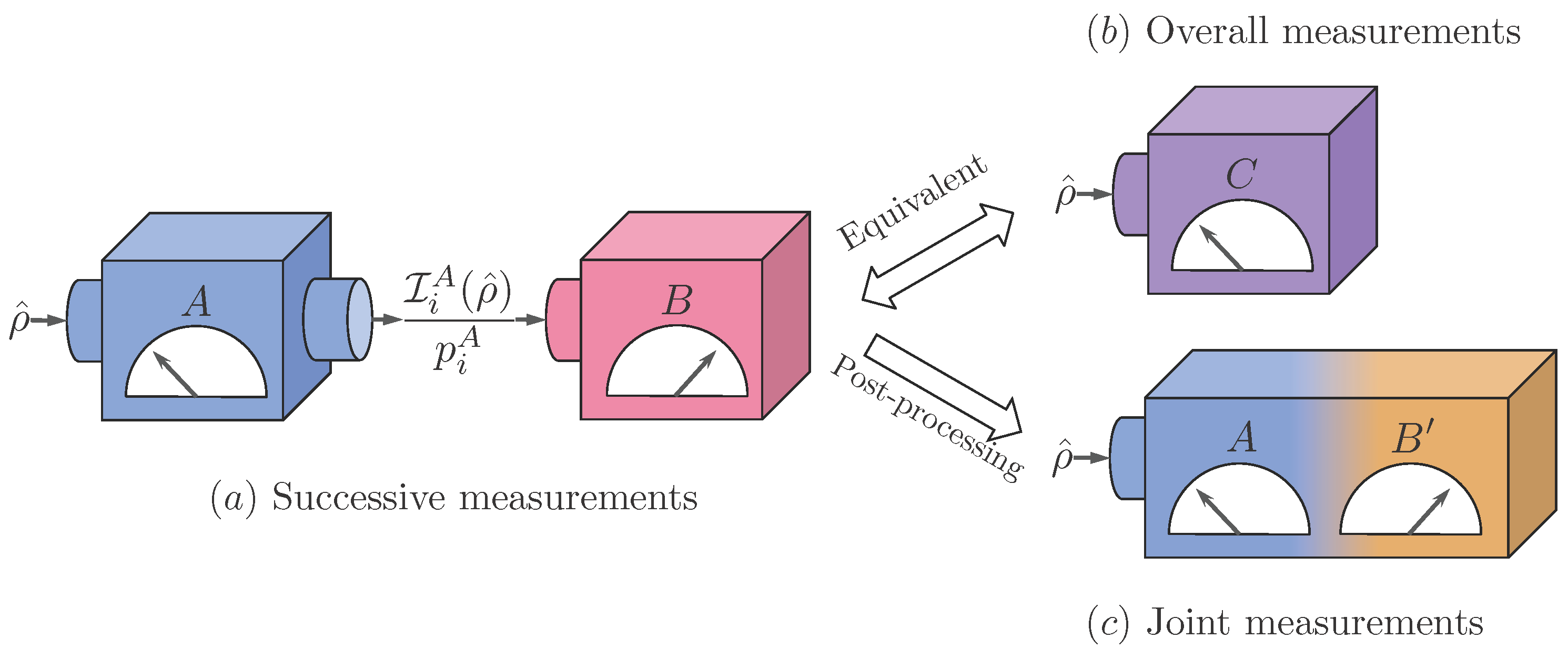
In the previous section, the mathematical methods have been presented, which are necessary to describe successive measurement in general. Based on the methods, we derive entropic uncertainty relations within the first scenario. As mentioned in
Section 2.2, we can consider performing successive measurement of
A and
B as a method to implement the corresponding overall measurement of
C. This fact implies that uncertainty existing in this scenario can be equivalently characterized as entropy of
C,
since
for all
i,
j. In other words, our goal to analyze uncertainty existing in the first scenario can be achieved under consideration of the overall observable
C. From this point of view, one can identify that the reason why we cannot avoid uncertainty in this scheme originates from intrinsic unsharpness of the overall observable
C. By quantitatively formulating this fact, as described in Equation (
5), we obtain entropic form of uncertainty relation lower bounded by device uncertainty characterizing unsharpness of
C such that
where state-independent bound
is obtained by minimizing device uncertainty of
C over all states. An important point here is that sequentially measuring incompatible observables may give rise to unavoidable unsharpness as the second measurement is disturbed by performing the first one. We can clearly observe the phenomena in the following cases.
3.1. Projective Measurement Model
In order to examine how much unsharpness emerges due to the incompatibility in the first scenario, let us consider successive projective measurements of observables
A and
B described by orthonormal bases
and
in
, respectively. Then, according to the state transformation
, this successive measurement can be considered as the overall measurement of
C, which is described by
for all
i,
j. In this case, by calculating the minimal value of device uncertainty defined in Equation (
5) we obtain
where the lower bound was proposed in [
12]. Here, it is notable that this bound is stronger than
, which is widely known as a measure of incompatibility [
15]. Thus, successively performing projective measurements of incompatible sharp observables induces unavoidable unsharpness which gives limits on one’s ability to measure with arbitrarily low uncertainty.
3.2. Lüders Instrument
As a generalized version of projective measurement model, let us assume that we implement the Lüders instrument for an unsharp observable
A at first and later a measurement of
B in the first scenario. In this case, each map
is fully determined by POVM element
as defined in Equation (
7), so that by applying adjoint map of
to each POVM element of
B such as Equation (
11), we obtain the explicit form of the overall observable
C described by
for all
i,
j. Then, it is straightforward to formulate relations among the concepts of uncertainty, unsharpness and incompatibility by directly using the relations in Equation (
5)
Here, the last inequality in Equation (
18) means that the minimal value of device uncertainty gives rise to a stronger bound than the incompatibility
c defined in Equation (
2). Therefore, as observed in the case of projective measurement model, one can identify that measuring incompatible observables by means of the Lüders instrument imposes the unavoidable unsharpness. In the following examples, we will analyze the relationships in Equation (
18).
3.3. Examples in Spin System
In order to clarify the relationship between
and
c and verify the validity of
for lower bound of uncertainty relation (18), let us consider an example of successively measuring two spin observables
Z at first and
later in
described by
respectively, where
and
are the Pauli spin matrices and unsharp parameters are denoted by
. Then the incompatibility of the observables is determined by
which is angle between directions of measurement components. Additionally, we assume that a
Z-compatible instrument is induced by a measuring process
, where an initial state of the probe system is
and a unitary operator
gives rise to a CNOT gate controlled by eigenstates of
,
and
. Namely, this measuring process leads to the Lüders instrument for
Z. In this case, the successive measurement scheme is equivalent to perform the overall measurement of
S defined in terms of four POVM elements
Calculating the device uncertainty for the overall observable
S, we obtain state-independent lower bounds
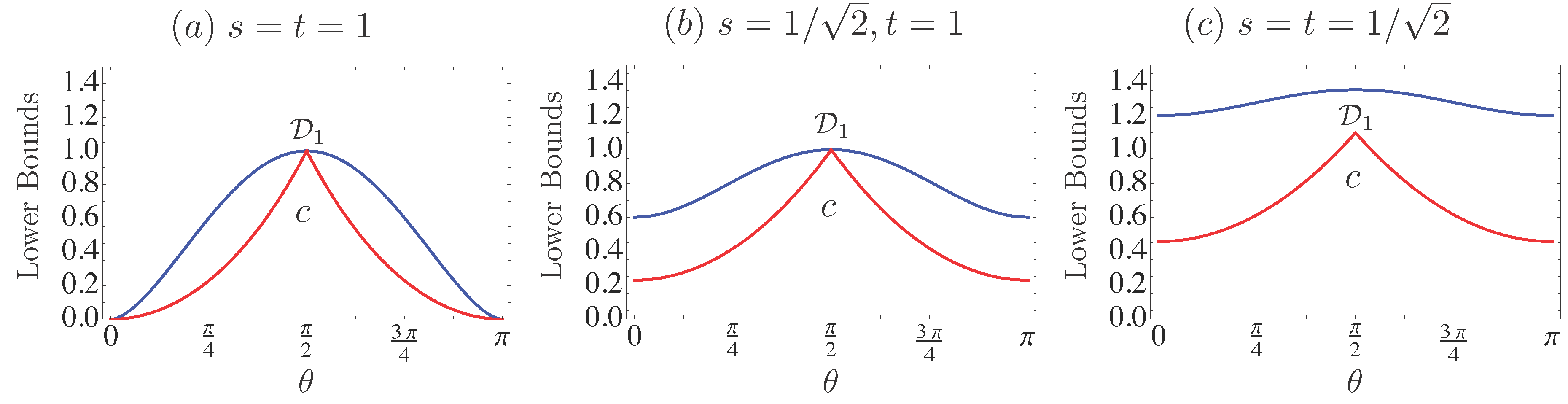
We plot the lower bounds
and
presented in Equation (
14) versus the angle
. As a result, we can check that
gives rise to strictly stronger bound than
c except when the spin components are mutually parallel or perpendicular in
Figure 2a. With increasing unsharpness of the observables, it becomes evident that
is well-formulated to reflect the effect of unsharpness as observed in
Figure 2b,c. In the examples, we analytically confirm the validity of
for a lower bound by comparing with
c, and, as a result, observe that measuring incompatible observables gives rise to unavoidable unsharpness originating from the incompatibility on the assumption that we implement the Lüders instrument in the first scenario.
4. Entropic Uncertainty Relations for a Jointly Measurable Pair of Observables Obtained via Successive Measurement Scheme
In this section, we consider entropic uncertainty relations for a pair of jointly measurable observables obtained via successive measurement scheme within the second scenario. As a first step, let us clarify the concept of a joint measurement. Given observables
A and
B, they are
jointly measurable if and only if there exists a
joint observable M composed of
-elements of POVM satisfying [
33]
Specifically, in the second scenario, the overall observable
C can be seen as a joint observable of
A and
by the definitions (12). Moreover, as mentioned in
Section 2.2, this scheme generally provides a method to implement joint measurements of any jointly measurable observables [
24]. Hence, entropic uncertainty relations obtained within this scenario is applicable to any pair of them.
Both observables
A and
obtained via the second scenario may have their own unsharpness, so that an amount of uncertainties about
A and
may not vanish due to the unsharpness of them. As formulating this fact, we obtain entropic uncertainty relations within the second scenario in the form of
where the sum of device uncertainties is written as
and thus minimizing it over all states can be accomplished by diagonalizing
and taking the lowest eigenvalue. An important point, here, is that the second measurement
B may be perturbed to be
because of disturbance caused by the first measurement
A, while
A is preserved. This fact implies that even when both observables
A and
B applied in this scheme are sharp, it is possible for the perturbed one
to become unsharp. In particular, this behavior is apparently observed when applying a pair of incompatible observables to this scenario, since measuring one of a pair of incompatible observables disturbs the other, according to the Heisenberg’s insight. From the point of view that the incompatibility imposes unavoidable unsharpness on the observables
A and
, we will discuss more details in the following specific measurement models.
4.1. Projective Measurement Model
In the same way in
Section 3.1, let us consider projective measurements of
A and
B described in
by orthonormal bases
and
, respectively. Then, in the second scenario, the first one
A remains itself, while the second one
B is disturbed to be
described by
for all
j. According to the Lüders theorem [
34],
B is not disturbed if and only if all elements of
A and
B commute each other. In this case, thus, even though we perform two sharp observables sequentially, the second one involves the unavoidable unsharpness originating from the incompatibility between them. This behavior can be quantitatively formulated in the form of
where its lower bound was proposed in [
12]. A generalized version of it for POVMs will be taken into account in the following.
4.2. Lüders Instruments
As a next step, in the same manner as
Section 3.2, let us assume we sequentially implement the Lüders instrument of an observable
A at first and later another one of
B, in the second scenario. Then, according to Equation (
7), it is equivalent to implement joint measurement of a pair of observables
A and
described by
for all
i,
j, respectively. In this case, likewise as discussed above, performing the Lüders instrument of
A gives rise to disturbance to
B, in a way for
B to become
. Then, by applying the relations in Equation (
5) directly, we obtain
where the last inequality follows from applying the third inequality in Equation (
5) solely to the observable
and its bound is a new form of incompatibility larger than
, which was conjectured in [
35] and proved later in [
36]. A distinct point from projective measurement model is that there is a possibility for
A to be unsharp, and loosing sharpness of
A may decrease disturbance to
B caused by
A. Namely, a trade-off between the unsharpness of
A and
B can be observed. In the following examples, this phenomenon will be examined.
4.3. Examples in Spin System
As an example in the second scenario, we assume to implement the Lüders instrument of
Z induced by the measuring process
and a measurement of
X successively in
described by
respectively. Here we restrict ourselves for
X to be sharp, in order to observe more clearly unsharpness appearing due to the first measurement. In this case, we can consider it as a method to measure a pair of jointly measurable observables
Z and
, where the perturbed observable
is given as [
37]
with the unsharp parameter
. Consequently, this scheme provides an optimized method to jointly measure incompatible observables
and
, in the sense that the unsharp parameters
s and
t saturate the inequality
, which is a necessary and sufficient condition for
Z and
to be jointly measurable [
38]. However, even in the optimized method, we can not avoid unsharpness, and there is the trade-off between the unsharpness of
Z and
such that the more sharpness of
Z, the more unsharpness of
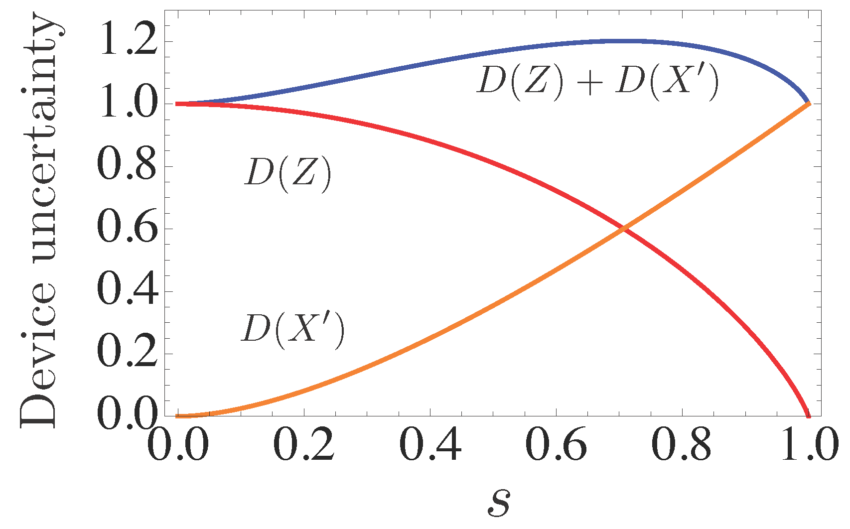
. This behavior can be examined quantitatively by considering entropic uncertainty relations (4) given in the form of
where binary entropy is denoted by
. The trade-off between the unsharpness of them is illustrated in
Figure 3, and the total unsharpness characterized by
is maximized when unsharpness equally distributed
, while minimized at extreme points
or
.
5. Conclusions
The main purpose of present work is to suggest entropic uncertainty relations for successive generalized measurement within two distinctive scenarios. Before deriving the relations, in
Section 2, we have introduced device uncertainty as a measure of unsharpness and its mathematical properties in order to investigate the effect of unsharpness on entropic uncertainty relations in successive measurement scheme. Subsequently, we have explicitly explained general description of successive measurement scheme with respect to two scenarios. In the first scenario, we have considered this scheme as a method to implement an overall measurement, and, as a result, observed that unsharpness of the overall observable gives limits on one’s ability to measure it with arbitrarily low uncertainty as formulated in Equation (
14). Assuming to perform the Lüders instrument as the first measurement in this scenario, it is clearly shown that this unsharpness comes from disturbance caused by the first measurement to the second one. The amount of unsharpness appears at least as much as the incompatibility of a pair of observables composing successive measurement, as formulated in Equation (
18). In the second scenario, on the other hand, this scheme has been considered as a method to measure a pair of jointly measurable observables. Consequently, we have figured out that total unsharpness in both observables is a major factor that gives rise to unavoidable uncertainty as observed in Equation (
24). Also, under the assumption for the first measurement to be described by the Lüders instrument, it becomes clear that the first measurement leads to unsharpness of the second one by disturbing it at least as much as incompatibility as shown in Equation (
29). It is notable that this form of uncertainty relations is applicable to any pair of jointly observables, since Heinosaari
et al. have proved that we can obtain any pair of jointly measurable observables via successive measurement scheme in [
24].


