1. Introduction
According to [
1], the main scope of mathematical modeling in epidemiology is “to develop models that will assist the decision-making process by helping to evaluate the consequences of choosing one of the alternative strategies available. Thus, mathematical models of the dynamics of a communicable disease can have a direct bearing on the choice of an immunization program, the optimal allocation of scarce resources, or the best combination of control or eradication techniques”. Starting from the seminal paper by Kermack and McKendrick [
2], a huge literature on dynamic models for infectious diseases has been produced as evidenced by the numerous books on the subject (see, e.g., [
3,
4,
5,
6,
7]). Mathematical models of epidemics usually consist of a system of differential equations governing the dynamics of the relevant state variables (susceptible, infective, recovered,
etc.). The differential equations can be ordinary, delay, partial or stochastic, according to the particular model or disease investigated. Equilibria and their stability, as well as the asymptotic behavior of the solutions are usually investigated.
A very interesting issue in the study of epidemic models is to identify therapeutic strategies that minimize the relevant negative features of the disease at the minimum cost. This naturally leads to the formulation and investigation of optimal control problems.
Confining ourselves to the epidemic compartment models, a typical optimal control problem consists of the minimization of the infected part of a population by the administration of a therapy to a part of the infected population. However, therapy is usually costly, and this poses a dilemma to the social planner.
The main tools to solve optimal control problems are a number of necessary and sufficient conditions characterizing the optimal solutions. Among the classical books on the optimal control theory, we cite [
8,
9]. More recently, optimal control monographs specifically oriented to the solution of biological and epidemic problems appeared (see, e.g., [
10,
11]).
The representation of the cost of a therapy is a key element in the formulation of the optimal control problem for the treatment of infectious diseases. For example, in the administration of a drug for a certain number of patients, the most natural way to introduce the cost would be
(monetary cost). However, in epidemic models, as well as in other economic applications, the cost is usually modeled by a function representing the cost as subjectively perceived by the decision-maker. This approach stems from the so-called utility theory, firstly introduced in a systematic way in the fundamental book [
12].
On the other hand, the choice of the cost function is often simply done to make the problem more tractable.
If we denote by the fraction of a population treated by some drug and by p the unitary cost of the therapy, then the (monetary) cost of the treatment should be . However, in many papers, that cost is simply represented by u or by without any reference to the price or to the number of people treated. This seems a little bit surprising and needs at least further investigation.
A specific problem is also given by extremely expensive therapies in the presence of a very high number of patients to be healed. To treat all infected patients would mean sometimes spending all or a very large part of the national budget allocated to health. this is the case, for example, of the treatment of hepatitis C virus (HCV) by a costly drug, such as sofosbuvir. Such a choice is impractical or, in other words, has a cost (in terms of utility) that is infinite. A cost function incorporating such characteristics may be appropriate in this case.
The rest of the paper is organized as follows. In
Section 2, we investigate the optimal treatment of an infected population in the simplest case of a two-class population (susceptible and infectious people), comparing the results coming from five different kinds of cost functions.
In
Section 3, we discuss a model for the treatment of the HCV virus using the
blowing-up cost function and illustrate the result by some numerical simulations.
All of the proofs of the theorems are placed in
Appendix B.
2. Comparing Different Cost Functions
In this section, we wish to highlight the role played by different cost expressions on the solutions of the optimal control problem. For this purpose, it seems appropriate to test various cost functions on the simplest epidemic model proposed in the literature: the Susceptible-Infective-Susceptible (SIS) model. This model is appropriate for certain types of bacterial diseases, such as gonorrhea and meningitis (see [
13]).
Let us consider a population of
N individuals, divided into two classes: the class
S of those who are healthy, but susceptible to contracting the infection, and the class
I of those who have contracted the infection and can transmit it to the susceptible individuals through interpersonal contacts. It is
. In order to make the problem simple and meaningful at the same time, we neglect the demographic processes and assume that the transmission coefficient is normalized to one, so that the dynamics of
S and
I is governed by the system of differential equations:
Adding the two equation in Equation (
1), we have
, so that
N is constant.
In the rest of this section, we are interested in the “worst” case in which the total population is infected. Hence, let us assume that:
Then
for any
It follows that:
System (
1) reduces to the scalar equation:
Equation (
2) has only one stable feasible equilibrium
.
Assume that a fraction
of the infected population is treated, at the time
t, by some drug. Then, some of the healed infectives become susceptibles again. System (
1) becomes:
where
measures the effectiveness of the treatment. Again, in Equation (
3), it is
, so that:
A social planner wishes to minimize the number of infectives at the minimum cost. Let us assume that, during any period of length
τ, the budget of the social planner for the total health expenses is given by
. The monetary cost of the treatment borne by the social planner is
, where
p is the cost of treating the entire population. Nevertheless, this cost is perceived through a cost function:
which is not decreasing in its arguments.
We solve the following optimal control problem:
The constants
,
and
could be considered as values that will balance the units of measurements and also indicate the importance of one type of aim over the others (see also [
14]). For the sake of simplicity, in this section, we assume
.
Equation (
4) turns into the following maximization problem:
subject to the constraints:
and:
In the rest of the section, we assume that:
so that Equation (
7) is always satisfied and can be left out.
We apply, in the subsequent analysis, the maximum Pontryagin principle (see Theorem 12 in the
Appendix).
Theorem 1 (Necessary conditions)
. Let be an admissible pair which solves Problems (5) and (6). Then, a continuous and piecewise continuously differentiable function exists, such that for all :for all , where H is defined by: Except at the points of discontinuities of , it is:where: Furthermore, the following transversality condition is satisfied: Note that:
and that Equation (
9) is equivalent to:
We consider five cost functions as listed below:
, linear state independent cost (LSI);
, linear state dependent cost (LSD);
, quadratic state independent cost (QSI);
, quadratic state dependent cost (QSD);
, blowing-up state dependent cost (BSD).
The LSI and especially QSI cost functions are very frequently used in the literature (see, e.g., [
15] LSI and [
16,
17,
18,
19,
20] QSI). They do not depend on the number of people treated, and this in some cases may sound rather strange. LSD and QSD cost represent linear and quadratic monetary costs, respectively. LSD costs are used, e.g., in [
21,
22].
A specific problem is given by extremely costly therapies in the presence of a very high number of patients to be treated. To treat all infected patients would mean sometimes spending all or a very large part of the national budget allocated to health. Such a choice is impractical or, in other words, has a cost (in terms of utility) that is infinite. The BSD cost function incorporates such characteristics. It approximates monetary costs when they are small and tends to infinity as the monetary costs approach the available budget.
We prove the following result:
Theorem 2. Let .If , then satisfies the maximum principle for Problems (5) and (6) if and only if: If , then it is never optimal to set , and then, .
Theorem 2 establishes that if the cost function is LSI, or LSD, or BSD, then it could be optimal to not treat any infected people provided that the ratio price/effectiveness is too high. By contrast, if the cost function is quadratic, then it is convenient to treat a positive fraction of the infected population at any time, no matter the price of the drugs nor their effectiveness.
Now, we characterize the optimal solutions by means of the maximum principle for the five different cost functions proposed above. In particular, we will establish conditions on the parameter, such that the treatment of the total infected populations is optimal at any time.
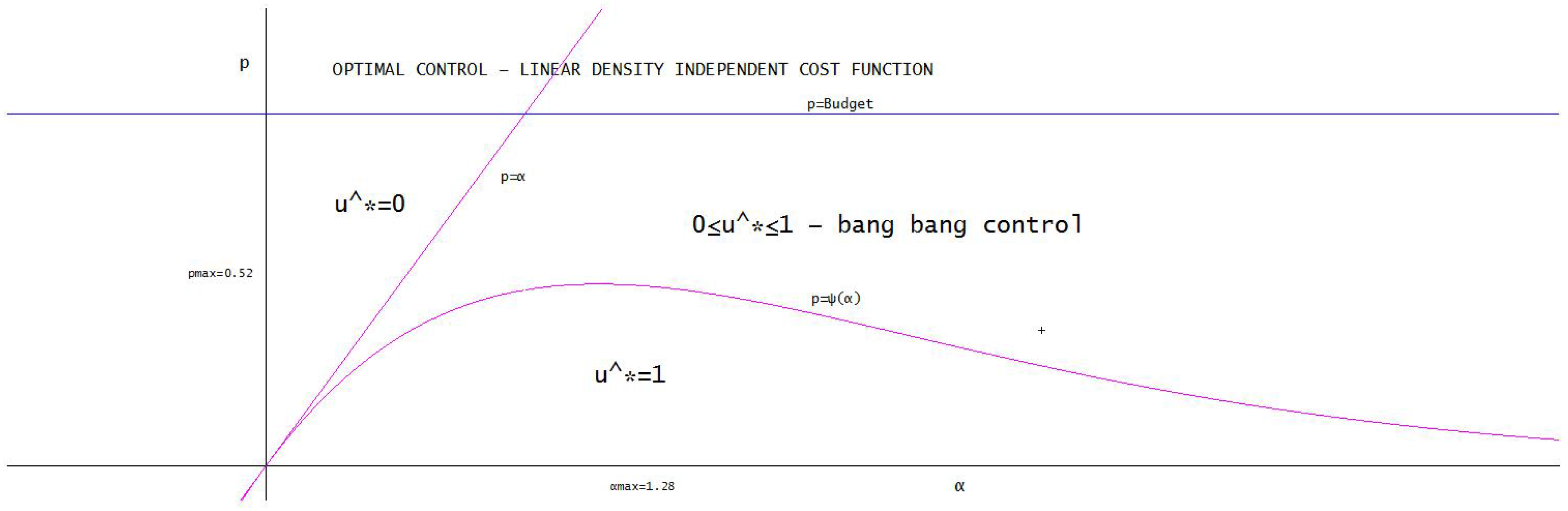
2.1. Linear Density Independent Costs
In this section, we assume that:
It follows from the maximum principle that:
The adjoint equation is:
with
Theorem 3. satisfies the maximum principle if and only if:where: A unique solution of the equation exists. Moreover: Figure 1 illustrates the different optimal policies with respect to the price
p and to the effectiveness
α.
2.2. Linear Density Dependent Costs
In this section, we assume that:
The adjoint equation is:
with
Theorem 5. satisfies the maximum principle if and only if , for any .
If , we know from Theorem 2 that satisfies the maximum principle. Nevertheless, there is a value , such that for , there is also a bang-bang control, which satisfies the maximum principle and which turns out to be the optimal solution. For the sake of simplicity, we illustrate this point confining ourselves to the case .
The linear density independent LDI and linear density dependent LDD cost function cases exhibit interesting differences. In both cases, it is optimal to not treat at all the infective population provided that p is large enough, that is treatment is too costly. If , then in the LDD case, it is optimal to treat the total infective population, while in the LDI case, this is true only if . The reason lies in the fact that the cost of the treatment (in terms of utility function) is taken as in the LDI case and in the LDD case. Since , it follows that .
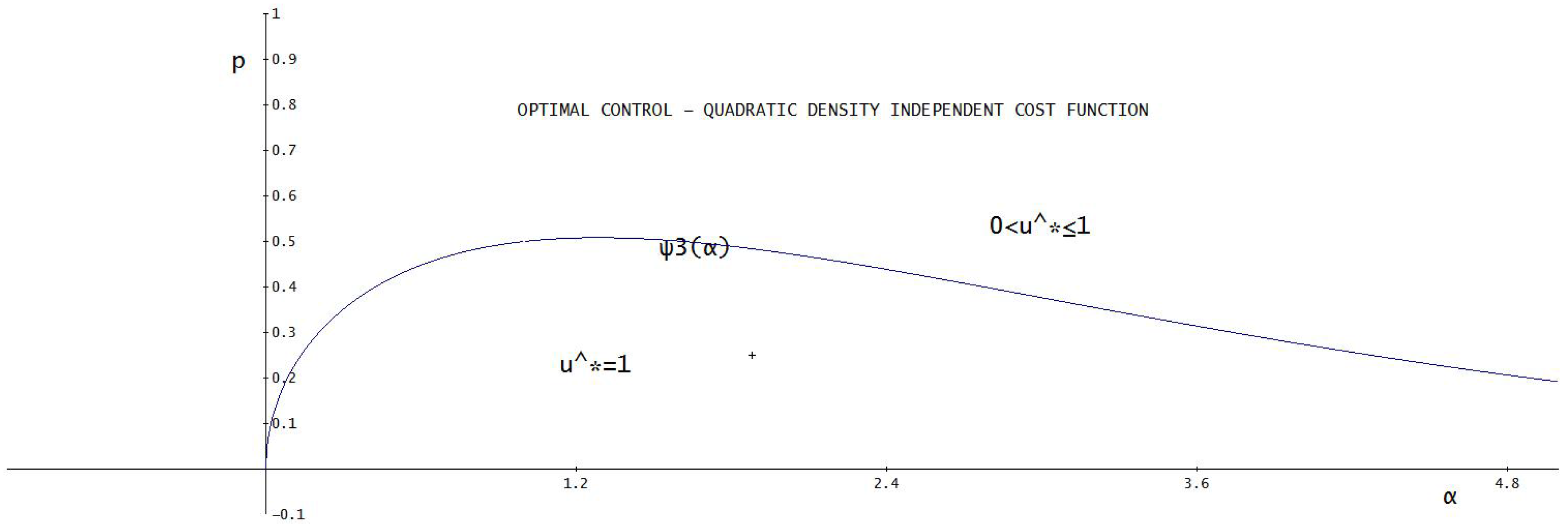
2.3. Quadratic Density Independent Costs
In this section, we assume that:
The adjoint equation is:
with
Since from Equation (
18), it can be proven that
for any
, it follows that
for any
. Therefore, it is never optimum to set
. It follows that:
where:
Theorem 7. satisfies the maximum principle if and only if for any , where: Note that if and , where . For these values of α, the set of prices for which it is optimal to treat the whole infected population is larger in the case of QDI compared to the LDI case. The opposite happens when .
We conclude this section with the following:
Then, a unique solution of the equation exists. Moreover: Figure 2 illustrates the different optimal policies with respect to the price
p and to the effectiveness
α.
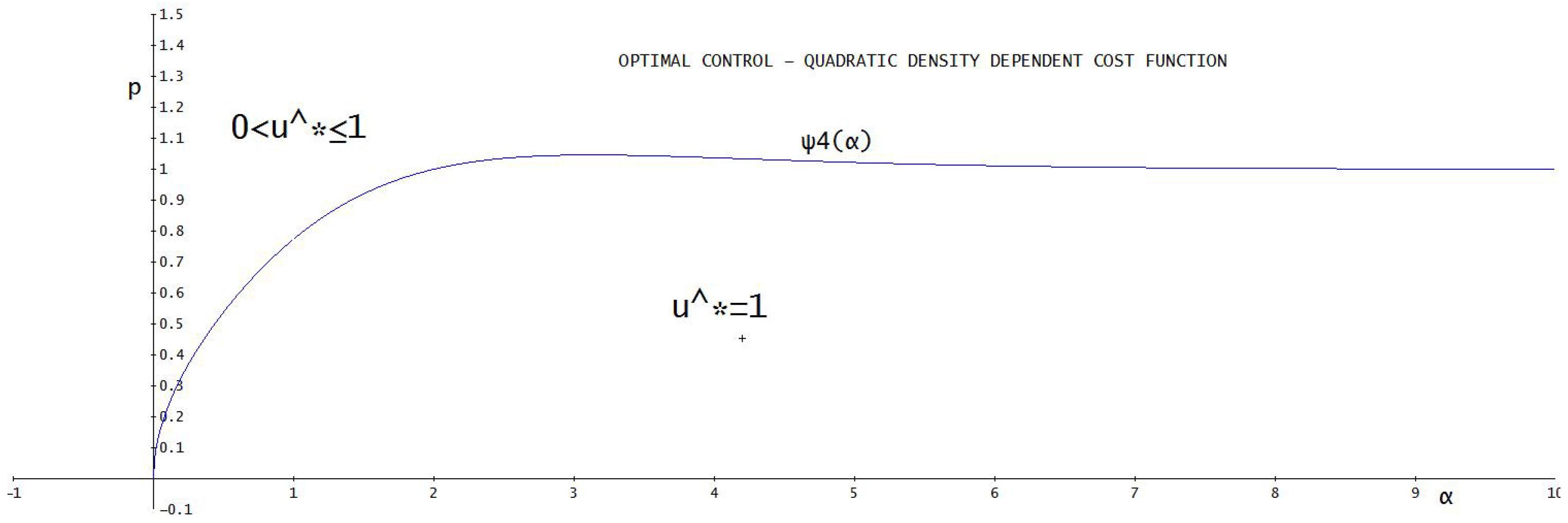
2.4. Quadratic Density Dependent Costs
In this section, we assume that:
The adjoint equation is:
with
Since from Equation (
19), it can be proven that
for any
, it follows that
for any
. Therefore, it is never optimum to set
. It follows that:
where:
Theorem 9. satisfies the maximum principle if and only if for any , where: Figure 3 illustrates the different optimal policies with respect to the price
p and to the effectiveness
α.
2.5. Blowing up Costs
As said above, to treat all infected patients would mean sometimes spending all or a very large part of the national budget allocated to health. Such a choice would have a cost (in terms of utility) that is infinite. A cost function incorporating such characteristics is the following one (note that if the monetary cost
is small, then:
):
The characterization of the case in which full treatment is optimal is, in principle, possible also in this case. However, due to the presence of one more parameter in the functional
J, the computations are really cumbersome. To make the results readable, we restrict our further analysis to the case:
Then satisfies the maximum principle if and only if: Note that is increasing and .
As an immediate consequence of the previous theorem, we have:
Remark 1. Assumption (
8) is necessary to obtain some of the results illustrated in the subsections above. If the price exceeds the budget, that is if
, then Theorem 2 still holds.
Moreover, it is never optimal to treat the entire population at any time. In fact at time , it is , so that the budget constraint requires . Hence, .
Let be characterized by and . It could be guessed that, if , then an optimal policy should be to use the entire budget for and then to switch to .
This is possible for all of the cost structure introduced above, except for blowing up costs. In such a case, in fact, to use the entire budget leads the cost function to infinity. Nevertheless, it can be easily proven that in the BSD case, if , then satisfies the maximum principle.
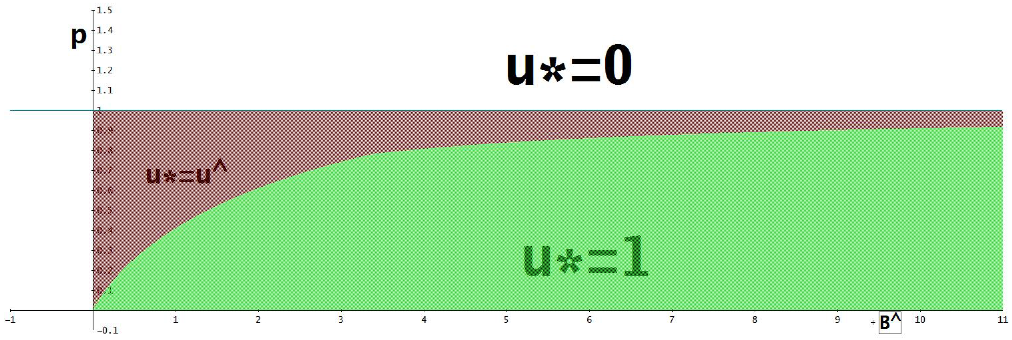
Remark 2. Note that Inequality (
20) does not provide an explicit dependence of
p with respect to the budget. Since
, it seems more meaningful to write Equation (
20) as:
Finally, Theorems 9 and 10 and Remark 1 are illustrated in
Figure 4.
3. The Hepatitis C Control
Let us consider a four-dimensional model with acute and chronic stages presented in [
23]. The epidemic is transmitted through people’s direct contacts. We suppose that the disease has an exposed period, and then, the patients enter into the acute stage, and finally, they undergo the chronic stage. The patients have no immunity after recovering and become susceptible again. We divide the population into four classes:
S-susceptible,
E-exposed,
I-infected with acute hepatitis C and
V-infected with chronic hepatitis C. The total number at time
t is
.
The basic assumptions are:
The birth rate of the population is , and the death rate is .
The disease cannot be transmitted during the exposure period.
Only the acute and chronic stages are differentiated. Patients with either acute or chronic infections are capable of transmitting the disease. Once a person contacts a susceptible individual, he or she must be infected.
Each acutely infective and each chronically infective makes and contacts per unit time, and then, the numbers of contacting susceptible individuals per unit time are, respectively, and . Hence, the incidences caused by acutely infective and by chronically-infective people are, respectively, and .
and are, respectively, the rate of progression to the acute stage from the exposed and the rate of progression to the chronic stage.
is the recovery rate for the chronic state.
The acute stage of infection is short and often asymptomatic, and there is no possibility for treatment during this state.
Since the disease-induced death rate is relatively low, it is ignored.
Under the assumptions above, we deal with the following model:
Summing the equations of System (
21), we obtain
. To simplify the subsequent analysis, we assume that:
Then,
N is constant in time, and we set
for each
. System (
21) becomes:
with initial conditions:
and:
Assume that a fraction
of the chronic infected individuals
V is treated at time
t. Then, a further progression from the class
V to the class
S occurs at a rate
, where
measures the effectiveness of the treatment. System (
22) becomes:
Let be the cost of treating the entire population, so that the monetary cost at time t for the treatment of the fraction of the chronic infected individuals V is given by .
The social planner wishes to minimize the infected population at the minimum cost. Let
be defined as in
Section 2. Obviously, it must be:
In the following, we assume that:
Hence, Equation (
23) is fulfilled for any
u and
V and can be dropped out. Let:
where
is the cost function in terms of the utility function. We assume that
is a non-negative smooth function and that it is increasing in its arguments.
A, B, C and D are the (non-negative) weights that the optimizer assigns to the different objects he or she wishes to maximize. It is . are the non-negative coefficients of the scrap values.
The government solves the following optimal control problem:
subject to Equation (
23) and with initial conditions:
An optimal control problem for the treatment of HCV virus is also investigated in [
24].
We characterize the optimal solution by using the maximum principle. The Hamiltonian
H is given by:
Since the treatment of the HCV-infected population is really expensive for the health social system, it seems appropriate to model the cost function as a blowing-up function. Let:
The adjoint equations are given by:
with terminal conditions:
If
, then
; otherwise, the equation
has a solution:
Therefore, the maximum principle gives:
Numerical Experiments
In this section, we illustrate some numerical simulations of the solution of the optimal HCV treatment problem. We use a fourth-order Runge–Kutta solver for the system of differential equations.
In this scenario, we assume that initially, the total population is infected and is at the chronic stage. In order to emphasize the role of the treatment on the population dynamics, we neglect births and deaths setting .
The cost functional assigns the same weight to the objective of minimizing the number of exposed, acute and chronic individuals. The scrap values are equally weighted.
As we mentioned above, the treatment of some infectious diseases is extremely costly, and this is the case of hepatitis C, for example. Therefore, in our simulations, we assume that the treatment of the total infected population at the initial time would require the entire budget and a consequent infinite disutility for the social planner. Precisely, we assume:
If , then it is optimal to not treat any person, that is . The population remains at the equilibrium .
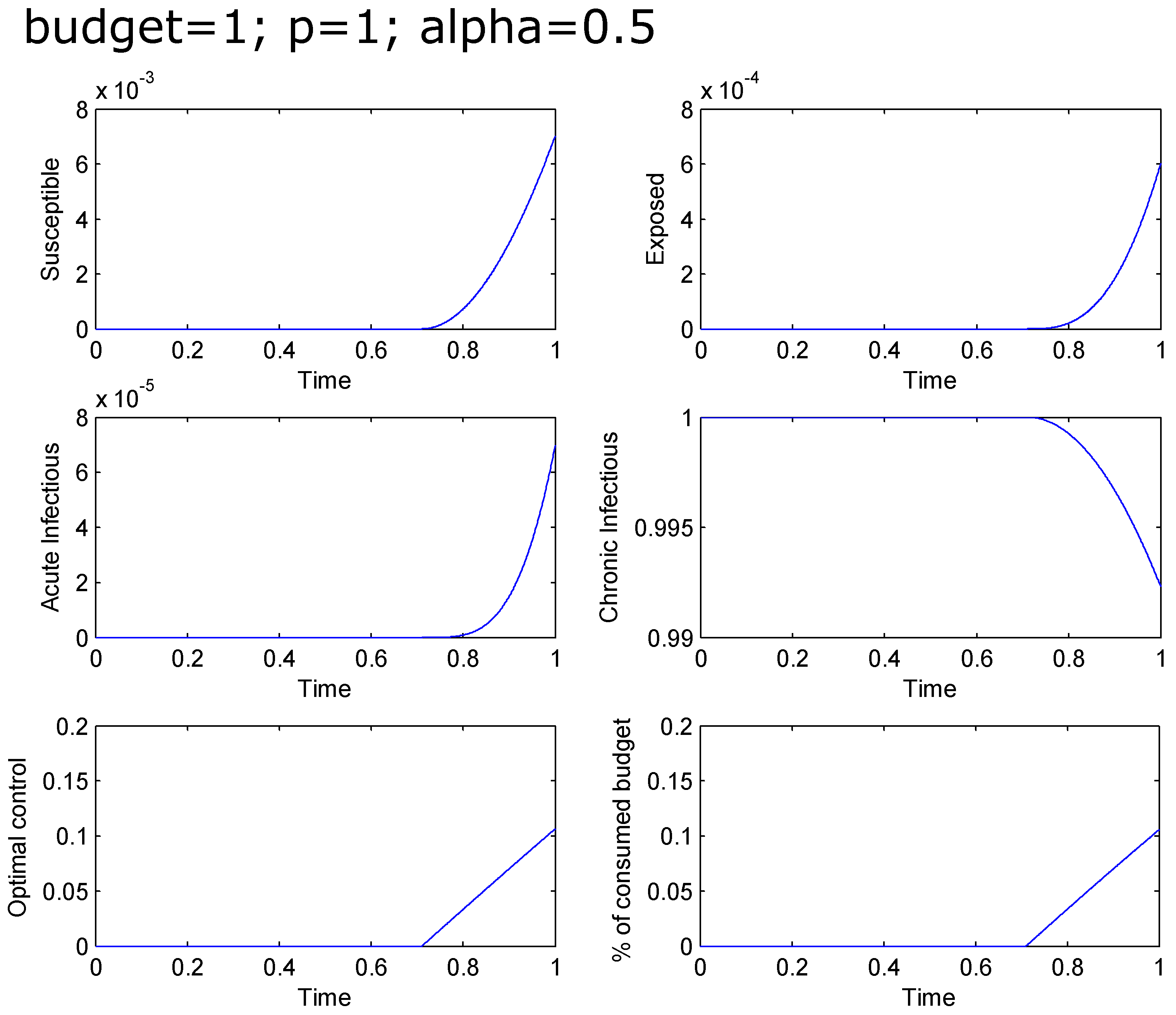
If
, then it is optimal to not treat any individual at the beginning and to start the treatment (and to increase it in time) at a time
, reaching at the final time
the
of the chronic population treated. The total infected population at the final time is greater than
. The percentage of the total budget used for the treatment goes from zero to
(see
Figure 5).
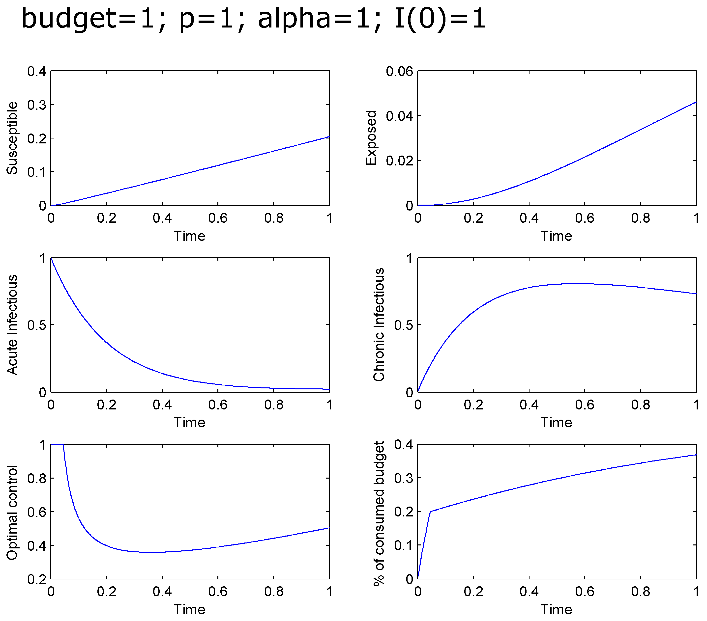
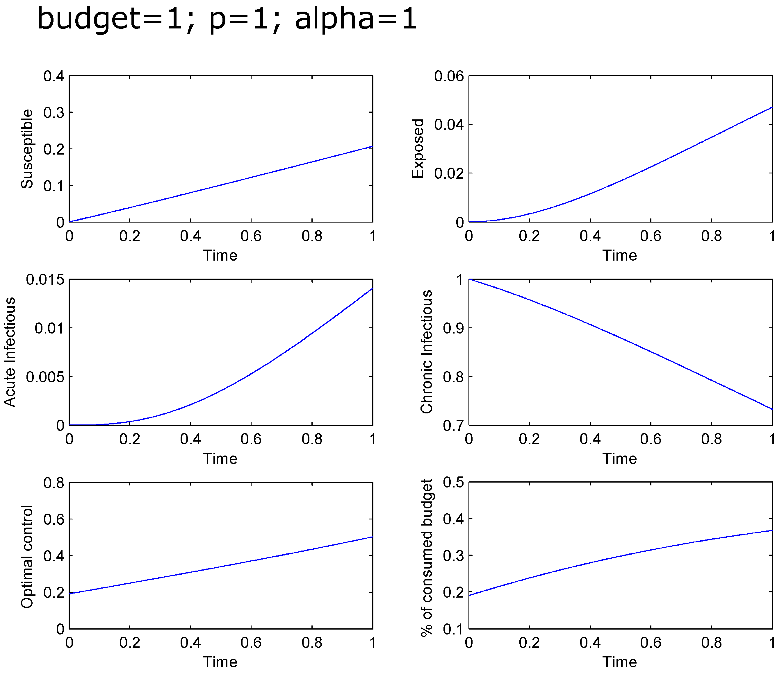
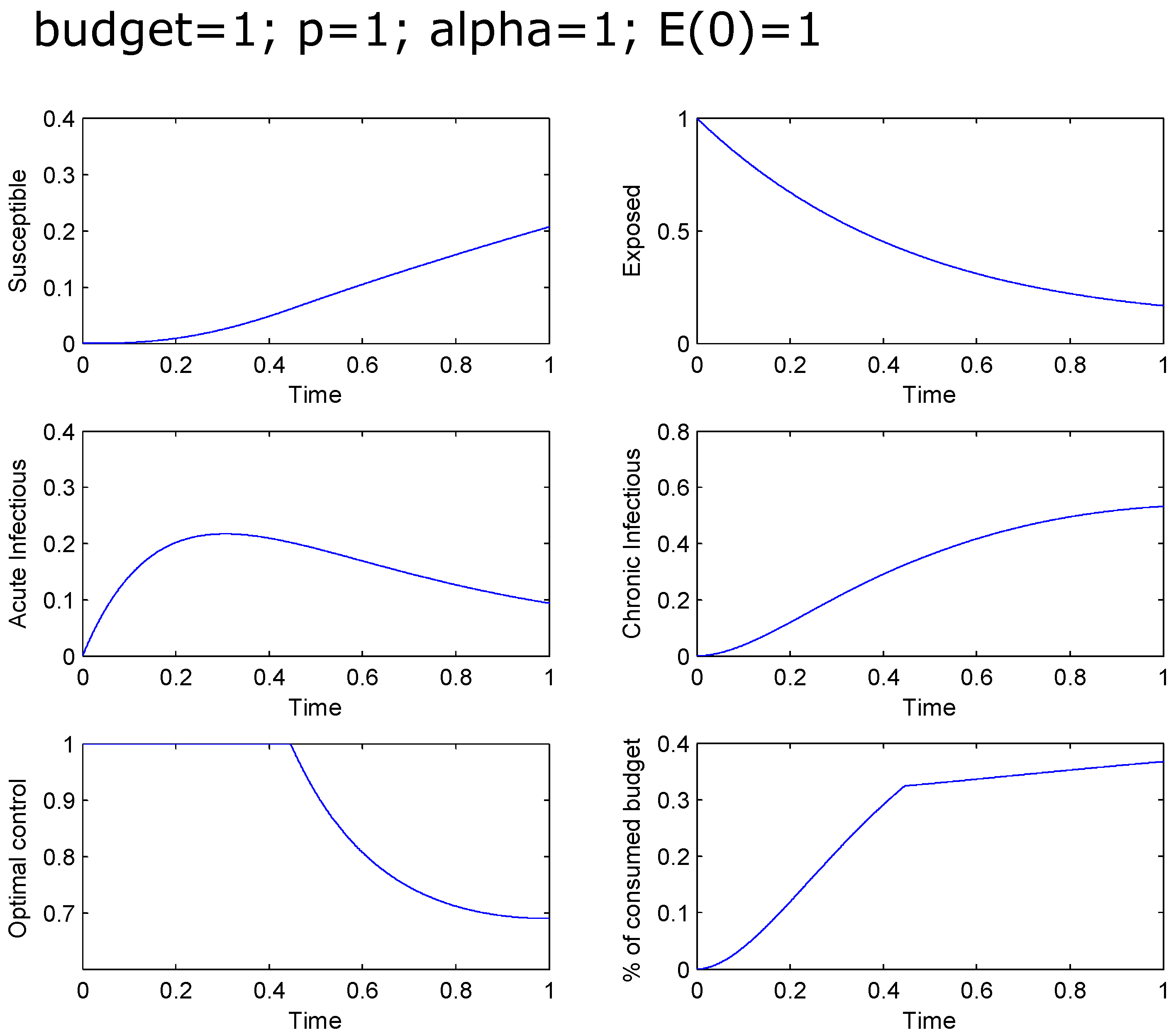
If the effectiveness
α is equal to one, then it is optimal to treat an increasing percentage of the chronic population, starting with
and terminating with
. The total infected population at the final time is around
. The percentage of the total budget used for the treatment goes from
to
(see
Figure 6).
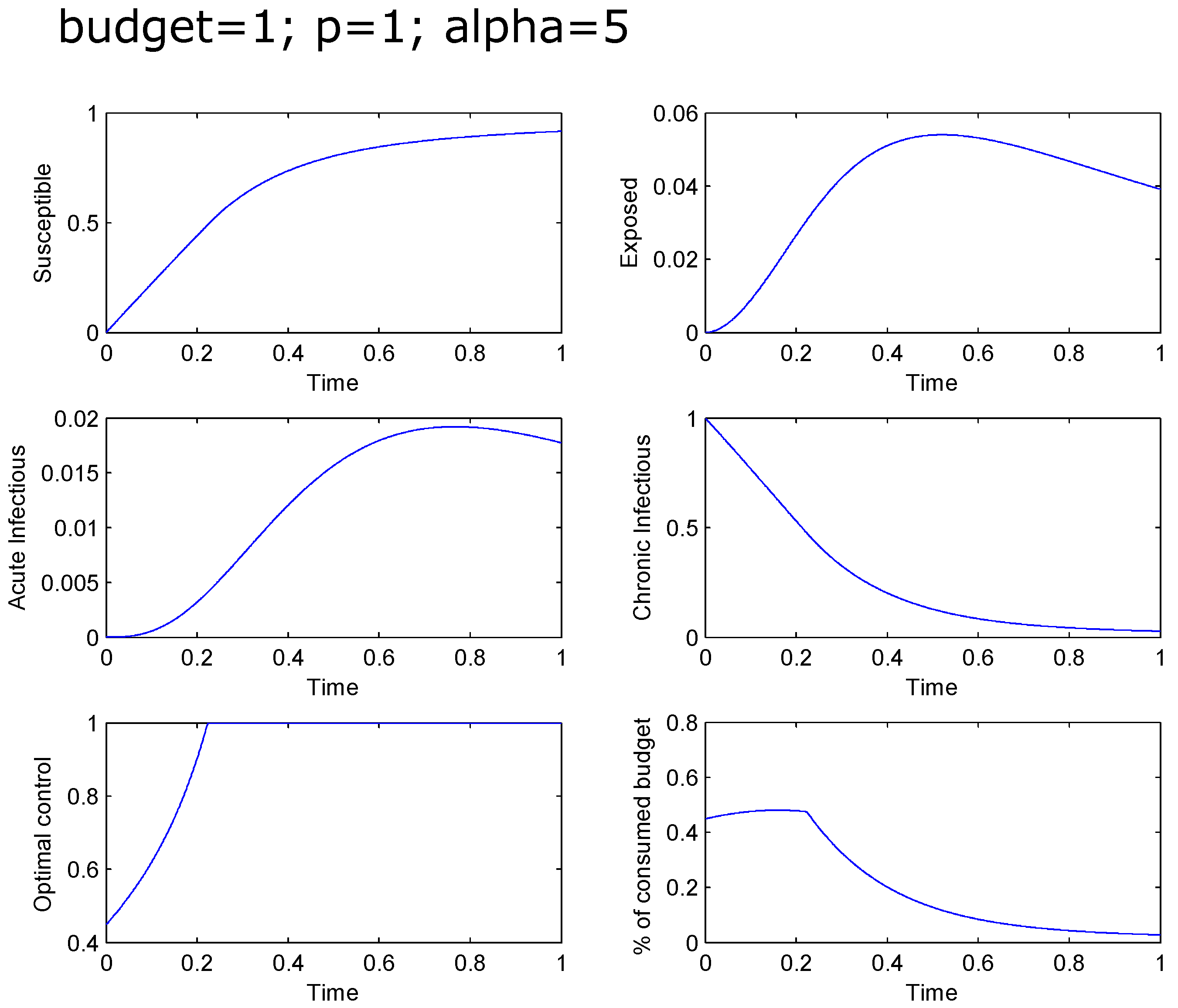
If
, then it is optimal to treat an increasing percentage of the chronic population, starting with
and treating the total chronic population after a short time (
). The total infected population at the final time is around
. The percentage of the total budget used for the treatment starts at
and approximates
at the end, reaching a maximum of around
at
(see
Figure 7).
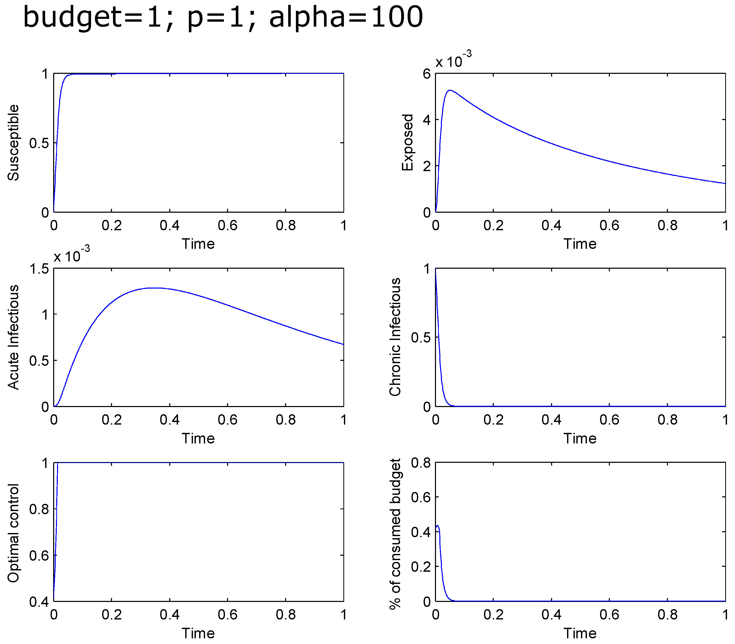
If
(that is extremely effective drugs), then the treatment of the total chronic population is still not immediate and starts after a very short time. The total infected population rapidly tends to zero while the percentage of the total budget used for the treatment starts at
and approximates zero at the end, reaching a maximum of around
(see
Figure 8).
Figure 9 and
Figure 10 illustrate again the case
, but with
and
, respectively.


