New Method of Randomized Forecasting Using Entropy-Robust Estimation: Application to the World Population Prediction

Abstract

We propose a new method of randomized forecasting (RF-method), which operates with models described by systems of linear ordinary differential equations with random parameters. The RF-method is based on entropy-robust estimation of the probability density functions (PDFs) of model parameters and measurement noises. The entropy-optimal estimator uses a limited amount of data. The method of randomized forecasting is applied to World population prediction. Ensembles of entropy-optimal prognostic trajectories of World population and their probability characteristics are generated. We show potential preferences of the proposed method in comparison with existing methods.

1. Introduction

For a studied process, forecasting as a procedure consists of four consecutive stages: modeling (model design), learning (estimation of model characteristics), testing (of the “learned” model) and prediction of future development.

Forecasting is based on retrospective data analysis with its subsequent extrapolation to future periods. Consider the state of a studied process at moment $t_0$, and suppose that the problem is to forecast further evolution of the process on a time interval ${\mathcal{T}}_{frc}=[t_0,T]$. Then, it is necessary to operate existing data on its past dynamics on a time interval ${\mathcal{T}}_{rts}=[T^{-},t_0]$, where $T^{-}<t_0$ (the so-called retrospective data). Generally, retrospective data and the time interval ${\mathcal{T}}_{rts}$ are divided into two groups, namely data serving for the estimation of the model’s characteristics (on a time interval ${\mathcal{T}}_{est}=[T^{-},t_e]$) and model testing (on a time interval ${\mathcal{T}}_{tst}=[t_e,t_0]$).

There exist at least three forecasting techniques differing in the objectification degree of constructed forecasts. The first technique, referred to as scenario forecasting [1], proceeds from the scenario approach whose objectification is replaced by the opinion of an expert group. Actually, it implements only the stages of modeling and prediction: learning and testing are eliminated owing to the opinion of experts, who choose an appropriate mathematical model of a studied process and form value sets (scenarios) of the model parameters. Then, the model with the scenario parameter values generates forecasting trajectories. As a matter of fact, such a forecasting technique is most widespread in demographic prediction [2,3,4]. Note that real retrospective data about a studied process are not utilized. They are indirectly reflected by the knowledge and experience of invited experts.

The second technique of forecasting explicitly involves real data for model learning and testing. The framework of mathematical statistics provides numerous estimation methods for model parameters; see [5,6,7,8]. Here, a major assumption is that the model possesses deterministic parameters, the values of which are defined using sets of real retrospective data. The latter are treated as a stochastic object with certain properties (a sample from a universe, normal distribution, etc.). In this case, one may assign different probabilistic characteristics (variances, confidence intervals, and so on) to the derived estimates of model parameters.

Sometimes, these characteristics assist in constructing the probabilistic characteristics of forecasting trajectories. The described technique will be termed probabilistic forecasting (PF) [9,10,11,12,13,14]. We emphasize that the above hypotheses regarding the stochastic properties of real datasets are almost impossible to verify, especially under small data arrays. It follows for the low efficiency of forecasts [15,16].

Finally, the third technique of forecasting proposed in this paper stems from the randomized model (RM) of a studied process, where model parameters are supposed random. Hence, we characterize RMs using the probability density functions (PDFs) of their parameters. At the learning stage, the PDFs of the model parameters are estimated on the basis of real retrospective data.

A randomized model generates an ensemble of forecasting trajectories, where each trajectory corresponds to a set of random realizations of parameters with the derived estimates of the PDFs. Computer simulation of such models employs the Monte Carlo method. Below, this technique will be called randomized forecasting (RF).

As opposed to existing methods [17,18,19], the proposed method of randomized forecasting is based on entropy-optimal estimations of PDFs for real datasets. The structure of the randomized dynamic model, used in this method, is based on ordinary differential equations.

The developed method serves for obtaining randomized predictions of the World population dynamics. Modeling the World population variations in time and space forms a major problem of demographic analysis [20,21,22].

Throughout the paper, we describe the above mentioned dynamics by the exponential model incorporating several parameters associated with fertility and mortality rates, as well as its change in time. In the randomized setting, they are assumed random, whereas World population is measured with random errors. To find the corresponding PDFs, the method involves the retrospective population data provided by the UN (see UNdata service at https://data.un.org/). In addition, we perform the comparative analysis of the PF- and RF-based approaches.

2. Randomized Model: Linear Differential Form

Consider a dynamic object having an input $\mathbf{f}(t)=\{f_1(t),\cdots ,f_m(t)\}$ and an output $\mathbf{x}(t)=\{x_1(t),\cdots ,x_n(t)\}$. The components of the input and output vectors can be observed (measured) on a time interval ${\mathcal{T}}_{rts}=[T^{-},t_0]$.

The relationship between the input and output of the object is described by the linear nonautonomous system of ordinary differential equations:

$$\begin{array}{c}\hfill \frac{d\mathbf{x}(t)}{dt}=A\mathbf{x}(t)+B\mathbf{f}(t),\mathbf{x}(T^{-})={\mathbf{x}}^0\end{array}$$

(1)

where $\mathbf{x}\in R^n$; $\mathbf{f}\in R^m,m\le n$; $A=[a_{ij}|(i,j)=\overline{1,n}]$ and $B=[b_{ik}|i=\overline{1,n},k=\overline{1,m}]$ denote matrices of appropriate dimensions.

The object’s output is observed with inevitable disturbances modeled by a vector noise $\overline{\xi }(t)=\{{\xi }_1(t),\cdots ,{\xi }_n(t)\}$. Therefore, the observed output of the model acquires the form:

$$\begin{array}{c}\hfill \mathbf{v}(t)=\mathbf{x}(t)+\overline{\xi }(t)\end{array}$$

(2)

where $\mathbf{v}(t)\in R^n$.

Equations (1) and (2) define a linear dynamical randomized model (LDRM) if:

• the matrix A is a random matrix (with independent random elements or elements with independent random components) of the interval type:

  $$\begin{array}{c}\hfill \mathcal{A}=[A:A^{-}\le A\le A^{+}]\end{array}$$

  (3)

  where $A^{-},A^{+}$ mean given matrices;
• there exists a probability density function (PDF) $P(A),A\in \mathcal{A}$;
• the vector $\overline{\xi }$ is a random vector (i.e., contains independent random components) of the interval type:

  $$\begin{array}{c}\hfill \Xi =[{\overline{\xi }}^{-}\le \overline{\xi }\le {\overline{\xi }}^{+}]\end{array}$$

  (4)
• there exists a probability density function (PDF) $Q(\overline{\xi }),\overline{\xi }\in \Xi$;
• the matrix B possesses fixed known elements.

Under the stated conditions, the LDRM generates an ensemble of random trajectories on the time interval $\mathcal{T}=[T^{-},T]$.

Let us rewrite the LDRM (2) in the input-output representation using the notion of matrix exponent [23]:

$$\begin{array}{c}\hfill W(A|t-\tau )=exp[A(t-\tau )]\end{array}$$

(5)

The input and output are measured at discrete moments with step h. Hence, on the time interval ${\mathcal{T}}_{est}$, we have:

$$\begin{array}{ccc}\hfill \mathbf{x}[T^{-}+ih]& =& W(A|ih){\mathbf{x}}^0+\hfill \\ & +& {\int }_{T^{-}}^{T^{-}+ih}W(A|T^{-}+ih,\tau )B\mathbf{f}(\tau )d\tau ,\hfill \\ & & i\in \overline{0,N_{est}}\hfill \end{array}$$

(6)

here $N_{est}=[(t_e-T^{-})/h]$ and $[•]$ indicates the integer part of •.

The LDRM output Equation (3) observed at discrete moments has the following form:

$$\begin{array}{c}\hfill \mathbf{v}[T^{-}+ih]=\mathbf{x}[T^{-}+ih]+\overline{\xi }[T^{-}+ih],i=\overline{0,N_{est}}\end{array}$$

(7)

Let us denote ${\overline{\xi }}^{(i)}=\overline{\xi }[T^{-}+ih],i=\overline{0,N_{est}}$. They are random vectors with independent and interval components. Now, we introduce the block-vector $\widehat{\xi }=\{{\overline{\xi }}^{(0)},\cdots ,{\overline{\xi }}^{(N_{est})}\}$. As we assume that these vectors and their components are independent, then the joint PDF is:

$$\begin{array}{c}\hfill Q(\widehat{\xi })=\prod _{i=0}^{N_{est}}{Q}_i({\overline{\xi }}^{(i)})=\prod _{i=0}^{N_{est}}\prod _{j=1}^n{q}_{ij}({\xi }_j^{(i)})\end{array}$$

(8)

The domain of this function is:

$$\begin{array}{c}\hfill \widehat{\Xi }=\underset{(N_{est}+1)\mathrm{multipliers}}{\underbrace{\Xi \times \Xi \cdots \times \Xi }}\end{array}$$

(9)

Here, $\overline{\xi }(T^{-}),\overline{\xi }(T^{-}+h),\cdots ,\overline{\xi }(T^{-}+N_{est}h)$ gives a sequence of n-dimensional independent random vectors of the interval type, associated with corresponding PDFs.

As soon as the matrix A and the noise vector $\widehat{\xi }$ are random and characterized by the PDFs $P(A)$ and $Q(\overline{\xi })$, respectively, so the observed output of the LDRM represents an ensemble $\mathcal{V}$ of random trajectories $\mathbf{v}[T^{-}+ih],i=\overline{0,N_{est}}$.

3. ${\mathcal{S}}_{\mathit{PQ}}^{\mathbf{1}}$ Entropy-Robust Estimation

The first stage of the randomized forecasting (RF) is an estimation of the PDFs of the RMs’ parameters and of the measurement noises. It is a classical problem of the Bayesian approach, and there exists the classical maximum likelihood method (or maximum relation of likelihood; see [6]) for its solving.

Let us recall the definition of the function of the relation of likelihood (FRL) in the terms of Section 2. The a priori PDFs $P^0(A),Q^0(\widehat{\xi })$ and the a posteriori PDFs $P(A),Q(\widehat{\xi })$ are the basic notations of the FRL. The FRL takes the form:

$$\begin{array}{c}\hfill L(A)=ln\frac{P(A)}{P^0(A)},L(\widehat{\xi })=ln\frac{Q(\widehat{\xi })}{Q^0(\widehat{\xi })}\end{array}$$

(10)

If the PDFs in these expressions are restored as functions of the parameters, then maximization of these functions gives “optimal” estimations. The principle of maximization of the FRL takes the form:

$$\begin{array}{c}\hfill \widehat{A}=arg\underset{A}{max}L(A)\end{array}$$

(11)

As a declaration, this principle is fine. However, how is it possible to restore the PDFs $P(A)$ and $P^0(A)$ (also $Q(\widehat{\xi })$ and $Q^0(\widehat{\xi })$)? The problem of the restoration of the PDFs remains outside of the FRL.

Let us consider the functional of the likelihood relation (FuRL) in the following form:

$$\begin{array}{c}\hfill \mathcal{L}[P(A)]={\int }_{\mathcal{A}}P(A)ln\frac{P(A)}{P^0(A)}dA,\mathcal{L}[Q(\widehat{\xi })]={\int }_{\widehat{\Xi }}Q(\widehat{\xi })ln\frac{Q(\widehat{\xi })}{Q^0(\widehat{\xi })}d\widehat{\xi }\end{array}$$

(12)

From Equation (12), we can see that the FuRL is the mathematical expectation of the FRL. On the other side, the FuRL is the opposite generalized information Boltzmann entropy (Kullback–Leibler distance) [24,25], that is:

$$\begin{array}{c}\hfill {\mathcal{H}}_A[P(A)]=-\mathcal{L}[P(A)],\mathcal{H}[Q(\widehat{\xi })]=-\mathcal{L}[Q(\widehat{\xi })]\end{array}$$

(13)

According to [26], maximization of entropy functions gives the best robust solution under high uncertainty. This idea with the addition of real data balance conditions forms the basis of the ${\mathcal{S}}_{PQ}^1$ entropy-robust estimation method [27].

The ${\mathcal{S}}_{PQ}^1$ entropy-robust estimation can be reformulated as a problem of functional nonlinear programming [28,29]:

$$\begin{array}{ccc}\hfill -\mathcal{H}[P(A),Q(\overline{\xi })]& =& {\int }_{\mathcal{A}}P(A)lnP(A)dA+\hfill \\ & +& {\int }_{\overline{\Xi }}Q(\widehat{\xi })lnQ(\widehat{\xi })d\widehat{\xi }\Rightarrow min\hfill \end{array}$$

(14)

subject to the constraints imposed on:

-

the class of (normalized) PDFs:

$$\begin{array}{ccc}\hfill & & {\int }_{\mathcal{A}}P(A)dA=1\hfill \\ & & {\int }_{\widehat{\Xi }}Q(\widehat{\xi })d\widehat{\xi }=1\hfill \end{array}$$

(15)

-

the balance between the first moment vector of the observed output $\mathbf{v}[T^{-}+ih]={\mathbf{v}}^{(i)}$ in the LDRM Equation (7) and the real data vector $\mathbf{y}[T^{-}+ih]={\mathbf{y}}^{(i)}$:

$$\begin{array}{ccc}\hfill \mathcal{M}\{{\mathbf{v}}^{(i)}\}& =& {\overline{\mathbf{v}}}^{(i)}[P(A),Q(\widehat{\xi })]={\int }_{\mathcal{A}}{\mathbf{u}}^{(i)}(A)P(A)dA+\hfill \\ & +& {\int }_{\widehat{\Xi }}{\overline{\xi }}^{(i)}Q(\widehat{\xi })d\widehat{\xi }={\mathbf{y}}^{(i)},i\in \overline{0,N_{est}}\hfill \end{array}$$

(16)

where:

$$\begin{array}{c}\hfill {\mathbf{u}}^{(i)}(A)=W(A|ih){\mathbf{x}}^0+{\int }_{T^{-}}^{T^{-}+ih}W(A|T^{-}+ih-\tau )B\mathbf{f}(\tau )d\tau \end{array}$$

(17)

${\mathcal{S}}_{PQ}^1$ entropy-robust estimation uses the first moment vector of the output LDRM. It is possible to use moments of higher order. This depends on measurable real data. If they represent the k-moment, then the balance condition can be formulated in the following form:

$$\begin{array}{c}\hfill {\left(\mathcal{M}\{{\mathbf{v}}^k\}\right)}^{1/k}=\mathbf{y}\end{array}$$

(18)

where ${\mathbf{v}}^{(k)}$ is a vector of k-moment components. In this case, we will have ${\mathcal{S}}_{PQ}^k$ entropy-robust estimation.

The problem Equations (14)–(17) are related to the Lyapunov problem [28,29] where the goal functional and constraints are of an integral type. Here, we will use the necessary condition of equality to zero of the integral equation:

$$\begin{array}{c}\hfill {\int }_{X}h(\mathbf{x})g(\mathbf{x})d\mathbf{x}=0\end{array}$$

(19)

where the function $h(\mathbf{x})$ is continuous and is equal to zero on the boundary of the set X (the class $\tilde{\mathcal{C}}$); the function $g(\mathbf{x})$ is differentiable (the class $\mathcal{D}$). Then, this equality will be valid for any function $h(\mathbf{x})$ with the mentioned properties if:

$$\begin{array}{c}\hfill g(\mathbf{x})=0,\forall \mathbf{x}\in X\end{array}$$

(20)

Now, we return to the problem Equations (14)–(17) and introduce the Lagrange functional:

$$\begin{array}{ccc}\hfill L[P(A),Q(\widehat{\xi })]& =& -\mathcal{H}[P(A),Q(\widehat{\xi })]+\lambda \left({\int }_{\mathcal{A}}P(A)dA-1\right)+\mu \left({\int }_{\widehat{\Xi }}Q(\widehat{\xi })d\widehat{\xi }-1\right)+\hfill \\ & +& \sum _{i=0}^{N_{est}}\langle {\overline{\theta }}^{(i)},{\mathbf{m}}^{(i)}[P(A),Q(\widehat{\xi })]\rangle \hfill \end{array}$$

(21)

where:

$$\begin{array}{c}\hfill {\mathbf{m}}^{(i)}[P(A),Q(\widehat{\xi })]={\overline{\mathbf{v}}}^{(i)}[P(A),Q(\widehat{\xi })]-{\mathbf{y}}^{(i)}\end{array}$$

(22)

Sign $\langle •,•\rangle$ denotes a scalar product.

As the solution of the problem Equations (14)–(17) is searched in the class of differentiable functions, then the Gato derivation can be used for determination of the variation of Lagrange functional Equation (21).

Let us denote the solution of the problem Equations (14)–(17) as $P^{*}(A)$ and $Q^{*}(\widehat{\xi })$. Furthermore, introduce the functions $\varphi (A)\in \tilde{\mathcal{C}},\psi (\widehat{\xi })\in \mathcal{D}$ and two scalar variables $\alpha ,\beta$ to present the functions $P(A),Q(\widehat{\xi })$ in the following form:

$$\begin{array}{c}\hfill P(A)=P^{*}(A)+\alpha \varphi (A),Q(\widehat{\xi })=Q^{*}(\widehat{\xi })+\beta \psi (\widehat{\xi })\end{array}$$

(23)

Functions $P^{*}(A),Q^{*}(\widehat{\xi })$, as a solutions of the problem Equations (14)–(17), are fixed. The optimality conditions for the problem Equations (14)–(17) take the form:

$$\begin{array}{c}\hfill {\left.\frac{dL}{d\alpha }\right|}_{\alpha =\beta =0}=0,{\left.\frac{dL}{d\beta }\right|}_{\alpha =\beta =0}=0\end{array}$$

(24)

The application of these conditions leads to the following systems of integral equations:

$$\begin{array}{ccc}\hfill {\int }_{\mathcal{A}}\varphi (A)\left(lnP(A)+1+\lambda +\sum _{i=0}^{N_{est}}\langle {\widehat{\theta }}^{(i)},{\mathbf{u}}^{(i)}(A)\rangle \right)dA& =& 0\hfill \\ \hfill {\int }_{\widehat{\Xi }}\psi (\widehat{\xi })\left(lnQ(\widehat{\xi })+1+\mu +\sum _{i=0}^{N_{est}}\langle {\overline{\theta }}^{(i)},{\overline{\xi }}^{(i)}\rangle \right)d\widehat{\xi }& =& 0\hfill \end{array}$$

(25)

According to Equations (19) and (20), we obtain the following equations, which are necessary optimality conditions (necessary conditions of Lagrangian-stationarity) for the problem Equations (14)–(17):

$$\begin{array}{ccc}\hfill lnP(A)+1+\lambda +\sum _{i=0}^{N_{est}}\langle {\widehat{\theta }}^{(i)},{\mathbf{u}}^{(i)}(A)\rangle & =& 0\hfill \\ \hfill lnQ(\widehat{\xi })+1+\mu +\sum _{i=0}^{N_{est}}\langle {\overline{\theta }}^{(i)},{\overline{\xi }}^{(i)}\rangle =0\end{array}$$

(26)

The solution of the problem Equations (14)–(17) takes the form:

$$\begin{array}{ccc}\hfill P^{*}(A)& =& \frac{exp\left(-{\sum }_{i=0}^{N_{est}}\langle {\overline{\theta }}^{(i)},{\mathbf{u}}^{(i)}(A)\rangle \right)}{\mathcal{R}\left({\overline{\theta }}^{(0)},\cdots ,{\overline{\theta }}^{(N_{est})}\right)}\hfill \\ \hfill Q^{*}(\widehat{\xi })& =& \frac{exp\left(-{\sum }_{i=0}^{N_{est}}\langle {\overline{\theta }}^{(i)},{\overline{\xi }}^{(i)}\rangle \right)}{\mathcal{Q}\left({\overline{\theta }}^{(0)},\cdots ,{\overline{\theta }}^{(N_{est})}\right)}\hfill \end{array}$$

(27)

where:

$$\begin{array}{ccc}\hfill \mathcal{R}\left({\overline{\theta }}^{(0)},\cdots ,{\overline{\theta }}^{(N_{est})}\right)& =& {\int }_{\mathcal{A}}exp\left(-\sum _{i=0}^{N_{est}}\langle {\overline{\theta }}^{(i)},{\mathbf{u}}^{(i)}(A)\rangle \right)dA\hfill \\ \hfill \mathcal{Q}\left({\overline{\theta }}^{(0)},\cdots ,{\overline{\theta }}^{(N_{est})}\right)& =& {\int }_{\widehat{\Xi }}exp\left(-\sum _{i=0}^{N_{est}}\langle {\overline{\theta }}^{(i)},{\overline{\xi }}^{(i)}\rangle \right)d{\overline{\xi }}^{(0)}\cdots d{\overline{\xi }}^{(N_{est})}\hfill \end{array}$$

(28)

The vectors of Lagrange multipliers are determined from the following equations:

$$\begin{array}{ccc}\hfill & & \mathbf{U}({\overline{\theta }}^{(0)},\cdots ,{\overline{\theta }}^{(N_{est})})={\int }_{\mathcal{A}}{\mathbf{u}}^{(i)}(A)\frac{exp\left(-{\sum }_{i=0}^{N_{est}}\langle {\overline{\theta }}^{(i)},{\mathbf{u}}^{(i)}(A)\rangle \right)}{\mathcal{R}\left({\overline{\theta }}^{(0)},\cdots ,{\overline{\theta }}^{(N_{est})}\right)}dA+\hfill \\ & +& {\int }_{\widehat{\Xi }}{\overline{\xi }}^{(i)}\frac{exp\left(-{\sum }_{i=0}^{N_{est}}\langle {\overline{\theta }}^{(i)},{\overline{\xi }}^{(i)}\rangle \right)}{\mathcal{Q}\left({\overline{\theta }}^{(0)},\cdots ,{\overline{\theta }}^{(N_{est})}\right)}d{\overline{\xi }}^{(0)}\cdots d{\overline{\xi }}^{(N_{est})}-{\mathbf{y}}^{(i)}=\mathbf{0},i\in [0,N_{est}]\hfill \end{array}$$

(29)

Calculation of the vectors ${\widehat{\theta }}^{*}=\{{\overline{\theta }}_{*}^{(0)},\cdots ,{\overline{\theta }}_{*}^{(N_{est})}\}$ is turned into a search for the global minimum of the residual function:

$$J(\widehat{\theta })={\parallel \mathbf{U}(\widehat{\theta })\parallel }_{L_2}$$

(30)

A global optimization algorithm is based on the simple Monte Carlo trials proposed in [30]. However, as soon as the $L_2$ metric is a convex function, one of the traditional gradient-based local optimization methods can be used for its solving.

4. Randomized Forecast Implementation

We comprehend a randomized forecast as an ensemble of trajectories on a forecasting interval ${\mathcal{T}}_{frc}=[t_0,T]$, which has to be generated using the model Equations (6) and (7) with the random matrix A and noise $\overline{\xi }$ described by the PDFs $P^{*}(A)$ and $Q^{*}(\overline{\xi })$, respectively; see formulas Equations (27) and (28). The matrices A and the vector noise $\overline{\xi }$ belong to the parallelepipeds $\mathcal{A}$ from Equation (3) and Ξ from Equation (4), respectively.

Let us study the generation problem of random matrices with the PDF Equation (27). First, we transform a matrix into a vector through concatenation of its rows. This procedure yields a vector $\mathbf{a}$ of length $m=n^2$. Additionally, the domain of random matrices becomes an m-dimensional parallelepiped:

$$\begin{array}{c}\hfill \mathbb{A}=[{\mathbf{a}}^{-}\le \mathbf{a}\le {\mathbf{a}}^{+}]\end{array}$$

(31)

where the vectors ${\mathbf{a}}^{-}$ and ${\mathbf{a}}^{+}$ result from the row concatenation of the matrices $A^{-}$ and $A^{+}$, respectively.

Lets consider a transformation of a vector $\mathbf{a}$ into a vector $\mathbf{q}$ belonging to the m-dimensional unit nonnegative cube $\mathbb{Q}$:

$$\begin{array}{c}\hfill \mathbf{a}=({\mathbf{a}}^{+}-{\mathbf{a}}^{-})\mathbf{q}+{\mathbf{a}}^{-},\mathbb{Q}=\{\mathbf{q}:\mathbf{0}\le \mathbf{q}\le \mathbf{1}\}\end{array}$$

(32)

Therefore, the entropy-optimal PDF undergoes the following chain of transformations:

$$P^{*}(A)\Rightarrow \mathbf{P}(\mathbf{a})\Rightarrow \mathbb{P}(\mathbf{q})$$

(33)

Therefore, it is necessary to generate random vectors $\mathbf{q}\in \mathbb{Q}$ with PDFs $\mathbb{P}(\mathbf{q})$. The generation was implemented by the acceptance-rejection algorithm [24].

5. Application of the RF Method for World Population Prediction

5.1. The World Population Prediction Problem

The state of an isolated population is characterized by its size $E(t)$ on a calendar time interval $\mathcal{T}=[T^{-},t_0]$. Population size varies under the impact of fertility and mortality processes, since World population is an isolated system. Within the framework of the linear population dynamics model, fertility and mortality are described by corresponding rates, whereas the flows of newborns and decedents appear proportional to population size, while fertility (b) and mortality (m) rates are considered as linear time-dependent parameters [22].

5.1.1. Randomized population model

World population evolves according to the following differential equation that has an analytical solution:

$$\begin{array}{ccc}\hfill \frac{dE(t)}{dt}& =& (b(t)-m(t))E(t),b(t)=b_0+u_{b}t,m(t)=m_0+u_{m}t\hfill \\ \hfill E(t)& =& E_{0}exp\left(\left((b_0-m_0)+\frac{1}{2}(u_b-u_m)t\right)t\right),\text{where}\hfill \\ \hfill E_0& =& E(T^{-}),b_0=b(T^{-}),m_0=m(T^{-})\hfill \end{array}$$

(34)

Real measurements of the population size dynamics modeled by Equation (34) take place at discrete moments. Hence, the population size at discrete moments $ih$ (where h specifies a given increment) is defined by the expression:

$$\begin{array}{ccc}\hfill {\Phi }_i(r,u_r|E_0)& =& E_{0}exp\left[(r+u_{r}i)ih\right],i\in I\hfill \\ \hfill r& =& b_0-m_0,u_r=\frac{1}{2}\left(u_b-u_m\right)h\hfill \end{array}$$

(35)

with parameters r and $u_r$, which describe the result of the difference between fertility and mortality flows.

World population is measured in billions of people. Fertility and mortality processes aggregate many factors, including measurement errors, whose quantitative analysis is impossible or complicated. On the other hand, the mass nature of fertility and mortality processes admits their modeling based on the probabilistic approach.

Thus, the resultant flow rate and its changing in time are supposed to be random variables with a joint probability density function $P(r,u_r)$ defined on the rectangle:

$$\begin{array}{c}\hfill \mathcal{J}={\mathcal{I}}_r\bigcup {\mathcal{I}}_{u_r},{\mathcal{I}}_r=[r^{-},r^{+}],{\mathcal{I}}_{u_r}=[u_r^{-},u_r^{+}]\end{array}$$

(36)

Generally, measurement errors are modeled by an additive noise $\xi [ih]$ of the interval type:

$$\begin{array}{c}\hfill \xi [ih]\in {\Xi }_i=[{\xi }_i^{-},{\xi }_i^{+}],i\in I\end{array}$$

(37)

where I indicates a time interval of such measurements. By assumption, the PDFs $q_i(\xi [ih]),i\in I$ are specified on the intervals ${\Xi }_i$ from Equation (37). Due to the independence of the set of random variables $\xi [0],\cdots ,\xi [ih]$, their joint PDF has the form:

$$\begin{array}{c}\hfill Q(\overline{\xi })=\prod _{i\in I}{q}_i(\xi [ih])\end{array}$$

(38)

Therefore, the randomized model of World population dynamics can be described by:

$$\begin{array}{c}\hfill v[ih]={\Phi }_i(r,u_r|E_0)+\xi [ih],i\in I\end{array}$$

(39)

where the function ${\Phi }_i(r,u_r|E_0)$ meets Equality (35).

5.1.2. Real and forecasting data

For PDF estimation, address the World population measurements for the period from 1960–1995 (http://data.un.org/; see

Table 1. Estimation interval ${\mathcal{T}}_{est}$.

i	0	1	2	3	4	5	6	7
year	1960	1965	1970	1975	1980	1985	1990	1995
${\mathit{E}}_{\mathit{real}}^{\mathit{est}}$	3.026	3.358	3.691	4.070	4.449	4.884	5.320	5.724

).

The entropy-optimal RM is tested via the measurements of the World population dynamics during the period from 1995–2015 and the values $E_{1985}^{prn}$ for this period (according to the UN forecast announced in 1985) (http://www.irbis.vegu.ru/repos/1002/Html/27.htm; see

Table 2. Testing interval ${\mathcal{T}}_{tst}$.

i	0	1	2	3	4
year	1995	2000	2005	2010	2015
${\mathit{E}}_{\mathit{real}}^{\mathit{tst}}$	5.724	6.128	6.514	6.916	7.359
${\mathit{E}}_{\mathbf{1985}}^{\mathit{prn}}$	5.666	5.962	6.450	6.985	7.469

).

The World population prediction till 2050 using the UN data is illustrated by

Table 3. Forecasting interval ${\mathcal{T}}_{frc}$

i	0	1	2	3	4	5
year	2015	2020	2025	2030	2040	2050
${\mathit{E}}_{\mathit{UN}}^{\mathit{frc}}$	7.359	7.644	7.964	8.284	8.924	9.564

(http://data.un.org/; [31]). United Nations’ projections both for the testing interval and the forecasting interval were made in accordance with the commonly-used cohort-component method, based on age-specific estimates of the components of population change (fertility, mortality and international migration) [32,33]. We will compare this prediction with its randomized analog.

World population is measured in billions of people. In the sequel, the subscript $real$ indicates the measured data of the population.

To summarize, the RM has the following forms on corresponding time intervals:

• on the estimation interval ${\mathcal{T}}_{est}$ (see Table 1):

  $$\begin{array}{c}\hfill v[ih]={\Phi }_i(r,u_r|E_{real}^{est}[0])+\xi [ih],i\in [0,7]\end{array}$$

  (40)
• on the testing interval ${\mathcal{T}}_{tst}$ (see Table 2):

  $$\begin{array}{c}\hfill v[ih]={\Phi }_i(r,u_r|E_{real}^{tst}[0])+\xi [ih],i\in [0,4]\end{array}$$

  (41)
• on the forecasting interval ${\mathcal{T}}_{frc}$ (see Table 3):

  $$\begin{array}{c}\hfill v[ih]={\Phi }_i(r,u_r|E_{real}^{frc}[0]),i\in [0,5]\end{array}$$

  (42)

where r and $u_r$ are random parameters with the entropy-optimal PDFs $P^{*}(r,u_r)$ and $\overline{\xi }$ is a vector of random noise with entropy-optimal PDF $Q^{*}(\overline{\xi })$.

5.1.3. The entropy-optimal PDFs of the parameters and noise

According to the general entropy-robust estimation procedure of PDFs (see Section 2), we have:

• the PDF of the parameters r and $u_r$ in the form:

  $$\begin{array}{c}\hfill P^{*}(r,u_r)=\frac{1}{\mathcal{R}(\overline{\theta }|E_{real}^{est}[0])}\prod _{j=0}^7{p}_j^{*}(r,u_r|{\theta }_j),p_j^{*}(r,u_r|{\theta }_j)=exp\left(-{\theta }_j{\Phi }_j(r,u_r|E_{real}^{est}[0])\right)\end{array}$$

  (43)
• the PDF of the noise in the form:

  $$\begin{array}{c}\hfill Q^{*}(\overline{\xi })=\frac{1}{\mathcal{Q}(\overline{\theta })}\prod _{j=0}^7{q}_j^{*}(\xi [jh]|{\theta }_j),q_j^{*}(\xi [jh]|{\theta }_j)=exp\left(-{\theta }_j\xi [jh]\right)\end{array}$$

  (44)

  where:

  $$\begin{array}{ccc}\hfill \mathcal{R}(\overline{\theta }|E_{real}^{est}[0])& =& {\int }_{\mathcal{J}}\prod _{j=0}^{7}exp\left(-{\theta }_j{\Phi }_j(r,u_r|E_{real}^{est}[0])\right)drd{u}_r\hfill \end{array}$$

  (45)

  $$\begin{array}{ccc}\hfill \mathcal{Q}(\overline{\theta })& =& \prod _{j=0}^6{\int }_{{\xi }_j^{-}}^{{\xi }_j^{+}}exp(-{\theta }_j\xi [jh])d\xi [jh]=\hfill \\ & =& \prod _{j=0}^6\frac{1}{{\theta }_j}\left(exp(-{\theta }_j{\xi }_j^{-})-exp(-{\theta }_j{\xi }_j^{+})\right)\hfill \end{array}$$

  (46)

To calculate the Lagrange multipliers, we will solve the system of balance equations (see Equations (16) and (17):

$$\begin{array}{ccc}\hfill & & \frac{1}{\mathcal{R}(\overline{\theta }|E_{real}^{est}[0])}{\int }_{\mathcal{J}}{\Phi }_i(r,u_r|E_{real}^{est}[0])\prod _{j=0}^{7}exp\left(-{\theta }_j{\Phi }_j(r,u_r|E_{real}^{est}[0])\right)drd{u}_r+\hfill \\ & +& \frac{1}{\mathcal{Q}(\overline{\theta })}{\int }_{\Xi }\xi [ih]\prod _{j=0}^{7}exp\left(-{\theta }_j\xi [jh]\right)d\xi [ih]-E_{real}^{est}[ih]=0,i\in [0,7]\hfill \end{array}$$

(47)

We will denote:

$$\begin{array}{c}\hfill {\mathcal{N}}_i(\overline{\theta }|E_{real}^{est}[0])={\int }_{\mathcal{J}}{\Phi }_i(r,u_r|E_{real}^{est}[0])\prod _{j=0}^{7}exp\left(-{\theta }_j{\Phi }_j(r,u_r|E_{real}^{est}[0])\right)drd{u}_r\end{array}$$

(48)

Then, Equation (47) can be rewritten as:

$$\begin{array}{ccc}\hfill {\mathcal{G}}_i(\overline{\theta }|E_{real}^{est}[0])& =& \frac{{\mathcal{N}}_i(\overline{\theta }|E_{real}^{est}[0])}{\mathcal{R}(\overline{\theta }|E_{real}^{est}[0])}+{\mathcal{L}}_i({\theta }_i)-y_i=0\hfill \\ \hfill y_i& =& E_{real}^{est}[ih],i=[0,7]\hfill \end{array}$$

(49)

where:

$$\begin{array}{c}\hfill {\mathcal{L}}_i({\theta }_i)=\frac{exp(-{\theta }_i{\xi }_i^{-})({\xi }_i^{-}+\frac{1}{{\theta }_i})-exp(-{\theta }_i{\xi }_i^{+})({\xi }_i^{+}+\frac{1}{{\theta }_i})}{exp(-{\theta }_i{\xi }_i^{-})-exp(-{\theta }_i{\xi }_i^{+})}\end{array}$$

(50)

We endeavor to solve these equations through minimizing the residual function:

$$\begin{array}{c}\hfill J(\overline{\theta })=\parallel \mathcal{G}(\overline{\theta })\parallel \Rightarrow min\end{array}$$

(51)

5.2. The Results of Computer Experiment

5.2.1. General conditions

We have performed calculations for the stages of estimation, testing and prediction with the following ranges for the model parameters, which include the possibility for both positive and negative trends of World population growth:

$$\begin{array}{ccc}\hfill {\mathcal{I}}_r& =& [-0.025;0.075],{\mathcal{I}}_{u_r}=[-0.002;0.001]\hfill \end{array}$$

(52)

and identically the range for the measurement noises:

$$\begin{array}{c}\hfill {\Xi }_j=[-0.5;0.5],j\in [0,7]\end{array}$$

(53)

Under the above ranges of the model parameters and measurement noises, the computer experiment has constructed the entropy-optimal PDFs and generated the ensembles of corresponding random trajectories for RM testing and randomized forecasting.

5.2.2. Estimation

On the estimation interval, we employ the data from Table 1. The residual function $J(\overline{\theta })$ Equation (51) is a function of eight variables, and it contains integral component Equations (45)–(49) to be estimated only numerically. For this, we have selected the so-called tiled method of two-dimensional integral estimation, which represents a combination of several quadrature formulas [34].

The idea of the tiled method consists of: (1) partitioning the whole domain of integration into a set of smaller-area subdomains having the rectangular or trapezoidal shape; and (2) applying appropriate quadrature formulas on each subdomain. The described method is implemented in MATLAB by the function quad2d.

Minimization of the residual function $J(\overline{\theta })$ (51) runs by the nonlinear trusted region method implemented by the function lsqnonlin from the package Optimization Toolbox. The function lsqnonlin has been optimized [35] for nonlinear least-squares problems.

The function lsqnonlin have several user-defined options for stopping criteria, such as function evaluation tolerance (${10}^{-6}$), step size tolerance (${10}^{-6}$) and maximum number of iterations (500).

Table 4. Calculated Lagrange multipliers.

Range ${\mathcal{I}}_r,{\mathcal{I}}_{u_r}$
Measurements	0	1	2	3	4	5	6	7
$\overline{\theta }$	0.0000	−0.3833	−0.3984	−0.5839	−0.3802	−0.4679	−0.1812	0.8881

presents the calculated Lagrange multipliers for the above ranges.

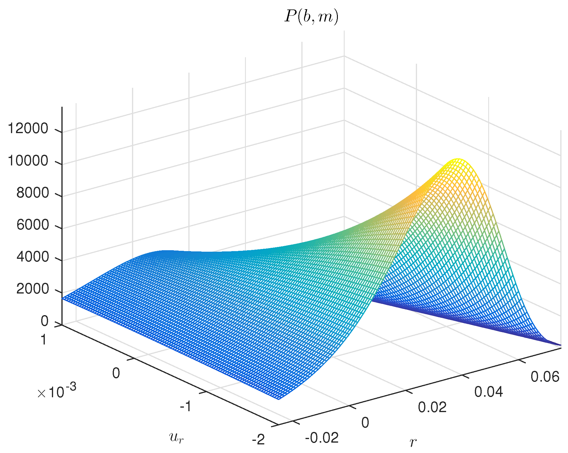
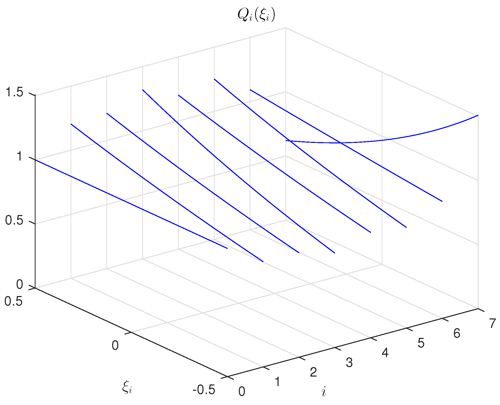
Figure 1 and Figure 2 demonstrate the entropy-optimal PDFs for the parameters of Model (35) and noise components. The functions $P^{*}(r,u_r,\overline{\theta })$ and $q^{*}(\xi [ih]),i\in [0,7]$ represent an entropy-optimal distribution of random variables at the corresponding intervals and will be used for making randomized predictions.

5.2.3. Testing

Testing of the model has been made using the data from Table 2. The population size has been evaluated by the Formula (41), where $r,u_r$ are the random variables with the PDF $P^{*}(r,u_r)$ and $\xi [ih]$ are the random noises with the PDFs $q_i(\xi [ih]),i\in [0,4]$ (see Figure 1 and Figure 2).

To generate an ensemble of random variables, the two-dimensional modification of the Ulam–von Neumann method has been used [24]. The size of the generated sample is $k=$ 100,000.

Each pair of the random values r and $u_r$ defines a separate exponential growth curve; moreover, for each point $ih$, a random value of the noise $\xi [ih]$ is added according to its PDF. As a result, the constructed trajectory of World population dynamics is not an exponential function.

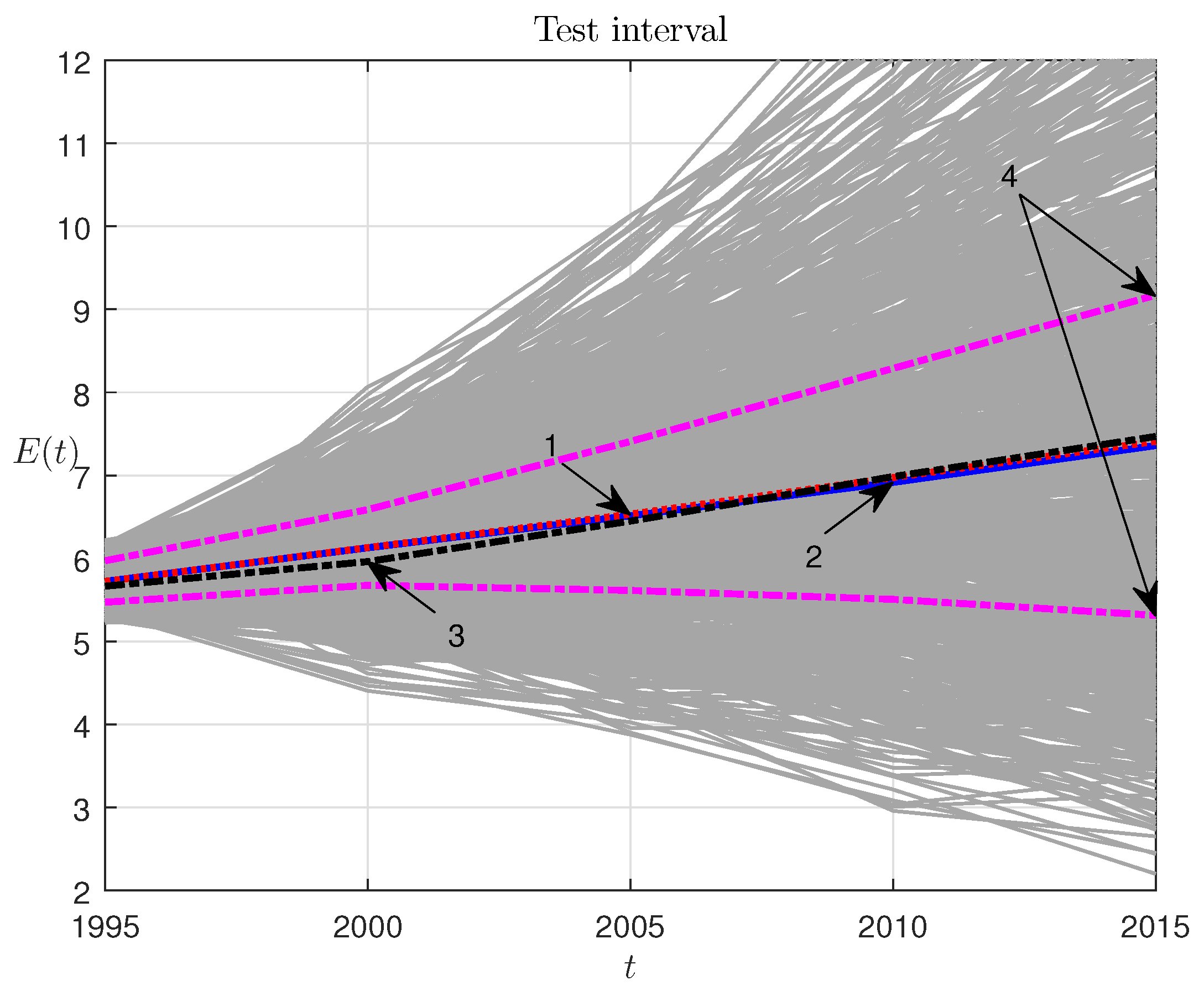
The test procedure yields the probabilistic characteristics of the parameters r,$u_r$ and ξ. It depends on the initial population size for the testing interval. Figure 3 shows the ensemble of the model-based trajectories for the parameter range from Equation (52) and the noise range from Equation (53), with a data-based selection of the initial point:

$$\begin{array}{c}\hfill E^{tst}[0]=E_{real}^{tst}[0]\end{array}$$

(54)

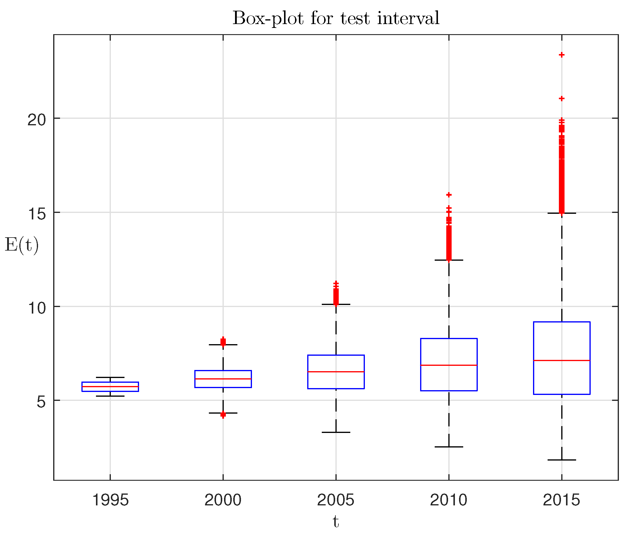
Figure 3 has the following notation: 1, the ensemble-average trajectories of population dynamics; 2, real population dynamics on the testing interval; 3, population dynamics on the testing interval according to the UN forecast of the year 1998; 4, the boundaries of the first and the third quartiles. The same model-generated ensemble for testing interval can be presented as a box plot with median mark and interquartile ranges; see Figure 4.

Testing quality is assessed by the root-mean-square error of the average trajectory with respect to its real counterpart:

$$\begin{array}{c}\hfill \delta =\parallel E^{tst}-E_{real}^{tst}\parallel =\sqrt{\sum _{i=0}^4{(E_{real}^{tst}[ih]-E^{tst}[ih])}^2}\end{array}$$

(55)

as well as by the relative error:

$$\begin{array}{c}\hfill \epsilon =\frac{\delta }{\parallel E_{real}^{tst}\parallel +\parallel E^{tst}\parallel }\end{array}$$

(56)

For instance, the UN forecast for the testing interval (Table 2) has the following errors:

$$\begin{array}{c}\hfill {\delta }_{1985}=0.228,{\epsilon }_{1985}=0.008\end{array}$$

(57)

In our case, the deviation of the model-average trajectory from the real one (Figure 3) appears to be appreciably smaller and demonstrates the following errors:

$$\begin{array}{c}\hfill {\delta }_{RM}=0.079,{\epsilon }_{RM}=0.003\end{array}$$

(58)

5.2.4. Prediction

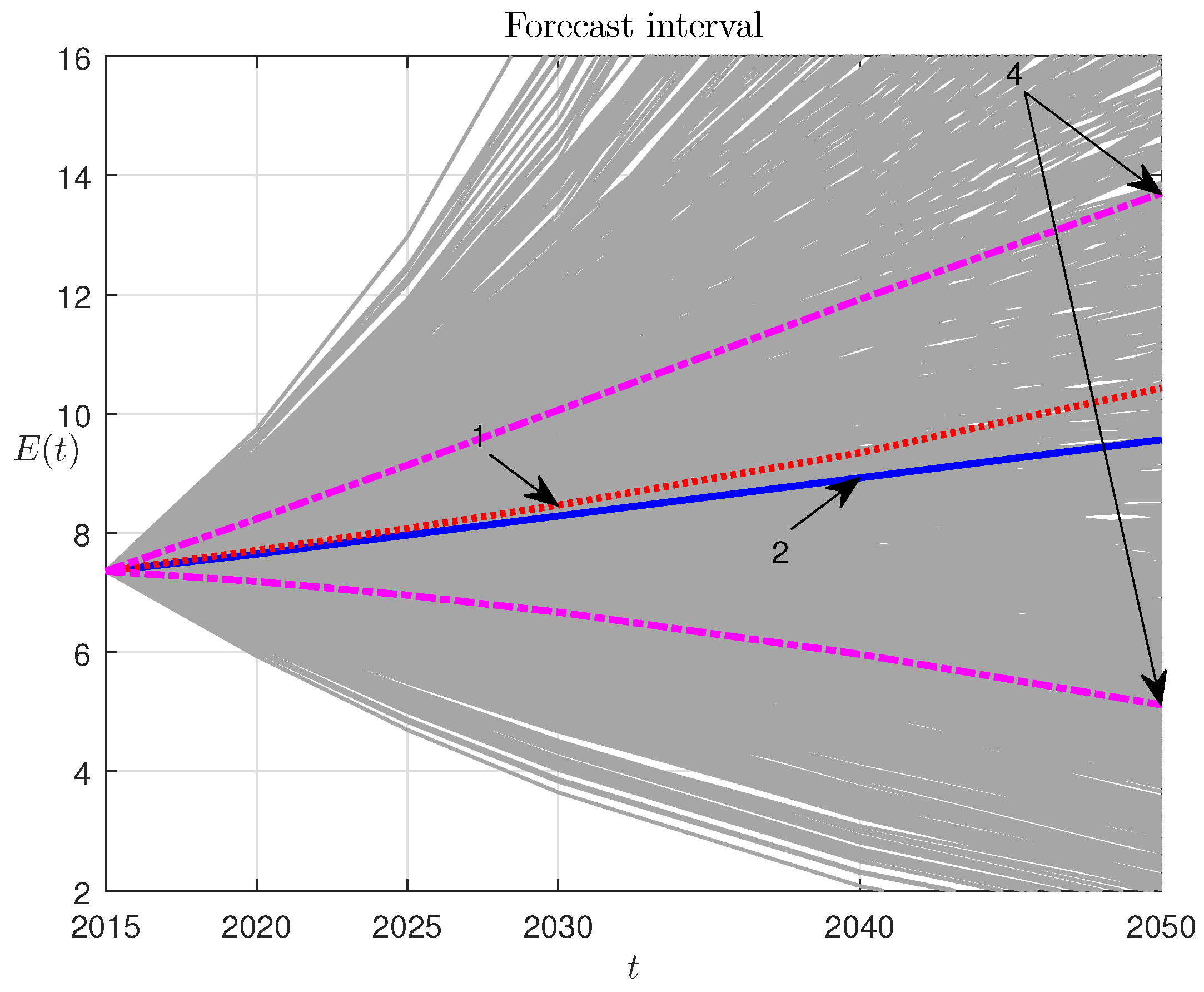
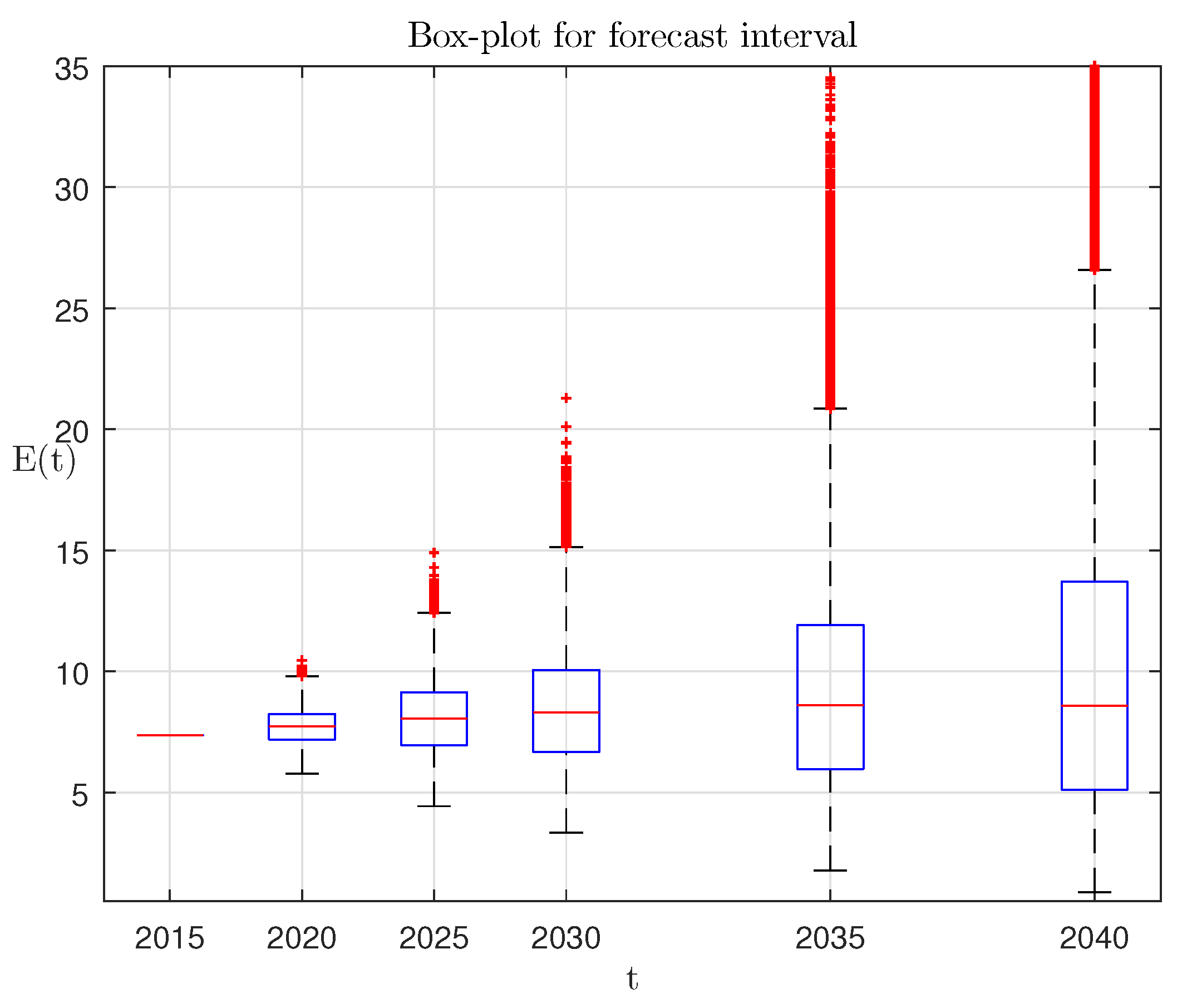
This simple RM has been applied to predict World population dynamics for the period from 2015–2050. The trajectory ensemble corresponding to the UN predictions (Table 3) is illustrated by Figure 5: 1, the ensemble-average trajectory; 2, UN projection; 4, the boundaries of the interquartile range (IQR zone). The corresponding box-plot is presented in Figure 6.

The presented results testify that the randomized forecasting as opposed to existent methods gives a set of probability characteristics of the World population prediction, which is calculated by using the ensemble of prognostic trajectories. The latter is generated by the randomized dynamic model with entropy-optimal PDFs of parameters. The randomized projection algorithm shows significantly closer to real data numerical results for testing interval, as well as stable projection that is higher, but close to the modern UN forecast for the future. According to our randomized model, 2026 will be the first eight billion year.

6. Conclusions

In this paper, we have suggested a randomized forecasting method that operates dynamic models described by linear ordinary differential equations with random parameters. Entropy-robust estimation has been developed for the probability density functions (PDFs) of model parameters and noisy measurements based on entropy maximization. It has been shown that the above PDFs belong to the exponential class. The randomized forecasting technique has been applied to randomized prediction of the World population dynamics. It has been demonstrated that randomized forecasting gives a set of probability characteristics of the World population dynamics.