Modeling ITNs Usage: Optimal Promotion Programs Versus Pure Voluntary Adoptions

Abstract

We consider a mosquito-borne epidemic model, where the adoption by individuals of insecticide–treated bed–nets (ITNs) is taken into account. Motivated by the well documented strong influence of behavioral factors in ITNs usage, we propose a mathematical approach based on the idea of information–dependent epidemic models. We consider the feedback produced by the actions taken by individuals as a consequence of: (i) the information available on the status of the disease in the community where they live; (ii) an optimal health-promotion campaign aimed at encouraging people to use ITNs. The effects on the epidemic dynamics of each of these feedback are assessed and compared with the output of classical models. We show that behavioral changes of individuals may sensibly affect the epidemic dynamics.

1. Introduction

Mosquito–borne diseases are diseases that are transmitted to humans and animals through the bite of an infected female mosquito. These include malaria, chikungunya, dengue, West Nile virus, Rift Valley fever, yellow fever and equine encephalitis. These diseases present major threats to human and animal health. For the malaria alone, it has been estimated that 3.3 billion people (almost half of the world’s population) are at risk of being infected and developing the disease, and 1.2 billion are at high risk [1].

Vaccine is often thought as a decisive tool against infectious diseases. Nevertheless, vaccines for mosquito–borne diseases are available only in a few cases (e.g., Japanese encephalitis and yellow fever [2]) whereas in most cases they are unavailable or developed only at experimental or trial levels. This is the case, for example, of chikungunya disease [3] and malaria [4]. A debated aspect of vaccine success concerns the effects, at population level, of mass administration of leaky vaccines (the ones that do not confer to the host both total immunity and incapability to transmit the disease). In case of malaria, for example, it has been speculated that using leaky vaccines may not reduce the malaria burden to an appreciable extent, and may cause increased rates of symptomatic malaria because it may have a detrimental effect on the naturally acquired immunity [5,6].

In view of effective vaccines development, a central role among the personal protection measures against mosquitoes is played by non-pharmaceutical interventions (NPIs). Such interventions are adopted to limit virus spread by reducing contacts between infectious and susceptible individuals [7]. Among the NPIs, the insecticide–treated bed–nets (ITNs) are a form of personal protection specifically targeted against mosquito-borne diseases transmission. In particular, it is nowadays recognized that ITNs are an effective method to reduce the malaria burden in endemic regions [8,9,10]. On the other hand, the effectiveness of ITNs is largely influenced by human behavioral factors. In fact, people may decide to not use ITNs, in spite of their usefulness, because of personal reasons [10]. Hot weather, a tendency to sleep outdoors and lack of mosquito nuisance are among the reasons for not using ITNs [11]. As a consequence, the role of human behavior (and misbehaviors) ought to be included in the modeling of ITNs–usage.

To this aim, we employ an approach in the framework of Behavioral Epidemiology, where a key issue is the assessment of the impact of human behavior on epidemics [12]. In particular, we propose a mathematical approach based on the idea of information–dependent epidemic models [12]. We employ as a basic model the one proposed in [13], where the dynamics of human and vector populations are described by two linked SIR epidemic models and the ITNs usage is represented by a constant coverage. We modify such a model to account of feedback produced by the actions taken by individuals as consequence of: (i) the information available on the status of the disease in the community where they live; (ii) an optimal health-promotion campaign aimed at encouraging people to use ITNs.

The main feature of the model presented here is the so–called information variable, as employed in [14,15,16,17,18].

We show that behavioral changes of individuals may sensibly affect the epidemic dynamics.

2. Models Formulation

2.1. The Basic System

The basic system we consider in this paper is the classical host–vector epidemic model in the version presented in [13], where the effects of ITN usage on the transmission of the disease is taken into account. The human and vector populations are divided into two disjoint compartments, given by susceptible and infectious individuals. Therefore, the state variables are given by: susceptible humans, $S_h$, infectious humans, $I_h$, susceptible vectors, $S_v$, and infectious vectors $I_v$. The dynamics is ruled by the following system of nonlinear ordinary differential equations:

$$\begin{array}{cc}{\dot{S}}_h=\hfill & {\Lambda }_h-{\lambda }_h\left(b\right)S_h-\mu S_h+\delta I_h\hfill \\ {\dot{I}}_h=\hfill & {\lambda }_h\left(b\right)S_h-(\alpha +\mu +\delta )I_h\hfill \\ {\dot{S}}_v=\hfill & {\Lambda }_v-{\lambda }_v\left(b\right)S_v-\eta \left(b\right)S_v\hfill \\ {\dot{I}}_v=\hfill & {\lambda }_v\left(b\right)S_v-\eta \left(b\right)I_v,\hfill \end{array}$$

(1)

where the upper dot denotes the time derivative. The terms ${\lambda }_h$ and ${\lambda }_v$ denote the forces of infection on humans and on vectors, respectively. That is, the per capita rate at which susceptible individuals contract the infection [19]. The infection rate per susceptible human and per susceptible vector are given, respectively, by:

$${\lambda }_h\left(b\right)=p_1\beta \left(b\right)\frac{I_v}{N_h},\mathrm{and}{\lambda }_v\left(b\right)=p_2\beta \left(b\right)\frac{I_h}{N_h},$$

(2)

where $\beta \left(b\right)$ represents the human–mosquito contact rate and the parameter $b\in [0,1]$ is the proportion of ITNs usage. The functions β and η are specified below. All the other parameters in System (1) are positive constants and their meaning is described in Table 1.

Table 1. Description of parameters in Model (1) and baseline values (taken from [13]).

Parameter	Description	Baseline Value
${\Lambda }_h$	Immigration rate in humans	${10}^3/(70\times 365)$
${\Lambda }_v$	Immigration rate in mosquitoes	${10}^4/21$
b	Proportion of ITN usage	varies in [0,1]
μ	Natural mortality rate in humans	$1/(70\times 365)$
η	Natural mortality rate in mosquitoes	$1/21$
${\eta }_{bn}$	Maximum ITN-induced death rate in mosquitoes	$1/21$
α	Disease–induced death rate in humans	${10}^{-3}$
$p_1$	Prob. of disease transm. from mosquito to human	1
$p_2$	Prob. of disease transm. from human to mosquito	1
${\beta }_{max}$	Maximum host–vector contact rate	0.1
${\beta }_{min}$	Minimum host–vector contact rate	0
δ	Recovery rate of infectious humans to be susceptible	1/4

Table 1. Description of parameters in Model (1) and baseline values (taken from [13]).

Parameter	Description	Baseline Value
${\Lambda }_h$	Immigration rate in humans	${10}^3/(70\times 365)$
${\Lambda }_v$	Immigration rate in mosquitoes	${10}^4/21$
b	Proportion of ITN usage	varies in [0,1]
μ	Natural mortality rate in humans	$1/(70\times 365)$
η	Natural mortality rate in mosquitoes	$1/21$
${\eta }_{bn}$	Maximum ITN-induced death rate in mosquitoes	$1/21$
α	Disease–induced death rate in humans	${10}^{-3}$
$p_1$	Prob. of disease transm. from mosquito to human	1
$p_2$	Prob. of disease transm. from human to mosquito	1
${\beta }_{max}$	Maximum host–vector contact rate	0.1
${\beta }_{min}$	Minimum host–vector contact rate	0
δ	Recovery rate of infectious humans to be susceptible	1/4

Using bed nets reduces the probability for humans to be bitten. Moreover, the nets are treated with insecticide. Therefore, in [13] the following two main assumptions are made:

(i) 

ITNs usage reduces the human–mosquito contact rate and this is described by the relation:

$$\beta \left(b\right)={\beta }_{max}-b\left({\beta }_{max}-{\beta }_{min}\right),$$

(3)

where ${\beta }_{max}$ and ${\beta }_{min}$ are the maximum and the minimum contact rate, respectively.

(ii) 

ITNs usage increases the mosquito death rate η. This is modeled by:

$$\eta \left(b\right)=\eta +{\eta }_{bn}b,$$

(4)

where ${\eta }_{bn}$ is a non negative constant and ${\eta }_{bn}b$ represents the death rate due to insecticide on treated bed-nets.

2.2. Information Variable

We propose an approach based on the idea of information–dependent epidemic models [12,14,15,16,17,18]. We begin by considering two different kinds of information available to the public:

(a)

the information on the status of the disease in the community where they live;

(b)

the information generated by an optimal health-promotion campaign aimed at encouraging people to use ITNs.

Generally speaking, the key point is that the information may potentially change the human behavior and this, in turn, generates a feedback effect on the disease spreading itself.

Our aim is to assess the feedback as produced by the actions taken by individuals as consequence of the information (a) or (b). We assume that the information available to the public is expressed in terms of a goodwill $w\left(t\right)$, which is analogous to the classical concept in marketing literature [20]. Here, w should be interpreted as concern or the willingness to use ITNs. Moreover, we introduce the information variable, as employed in [14,15,16,17,18]. That is to say, we assume that w depends on the past history in a way prescribed by a function ψ and distributed in the recent or far past by a delay kernel $K_{\xi }^p$. We set:

$$w\left(t\right)={\int }_{-\infty }^t\psi (S_h\left(\tau \right),I_h\left(\tau \right),S_v\left(\tau \right),I_v\left(\tau \right),u\left(\tau \right))K_{\xi }^p(t-\tau )d\tau .$$

(5)

In Equation (5) the function $u\left(t\right)$ (effort function) summarizes the actions taken by the public health authorities for promoting an health campaign (such as advertising, counseling, hygienic aid etc.). For any fixed time $T>0$, u is assumed to be a Lebesgue measurable function such that: $0\le u\left(t\right)\le u_{max}$ , for any $t\in [0,T]$.

The function ψ describes the information that individuals consider to be relevant for making their decision to adopt or not to adopt ITNs. In general, it will depend on the state variables (i.e., the environment’s status) and on the effort function u. The specific choice for this function will be presented later.

As in [18], the kernel $K_{\xi }^p$ is assumed to be an Erlangian kernel defined by the probability density function:

$$K_{\xi }^p\left(x\right)=\frac{{\xi }^p{x}^{p-1}{e}^{-\xi x}}{(p-1)!},x,\xi \in {\text{R}}_{+},p\in {\text{N}}_{+},$$

(6)

where $\xi >0$, $p=1,2,\cdots$ Therefore the delay is infinite and centered at the average delay $p/\xi$ [21].

Once that the goodwill has been introduced, we must now specify how it affects the forces of infection. We assume, as done in [20], that the contact rate decays exponentially with w, i.e., we consider the forces of infection given in Equation (2), where now $\beta \left(b\right)$ is replaced by:

$$\beta \left(w\right)={\beta }_{max}-ϵ\frac{{\beta }_{max}-{\beta }_{min}}{1-e^{-\gamma w_{max}}}\left(1-e^{-\gamma w}\right),$$

(7)

where γ is a positive constant and $ϵ\in \left\{0,1\right\}$ is a control parameter: $ϵ=0$ means that the contact rate is fully independent of the goodwill, whereas $ϵ=1$ indicates that the contact rate is information–dependent. In the latter case, observe that β in Equation (7) ranges from ${\beta }_{max}$ to ${\beta }_{min}$ as w ranges from 0 to $w_{max}$.

2.3. The Information Kernel

In Equation (6) we take $p=1$, so that $K_{\xi }^1\left(t\right)=\xi e^{-\xi t}$. This is the case of exponentially fading memory (or weak kernel). Note that the distribution mode is at $t=0$, whereas the average delay is at $t=1/\xi$. This means that the maximum information is on the current status of the “message” ψ, followed by a natural decay of the weighting, due for example to a fading public’s memory or the increasing disregard by the public for the message. In this case, from Equation (5), by using the linear chain trick [21] we have:

$$\begin{array}{cc}{\displaystyle \frac{dw}{dt}}\hfill & =\xi {\displaystyle \frac{d}{dt}\left[{\int }_{-\infty }^t\psi \left(\tau \right)e^{-\xi (t-\tau )}d\tau \right]}\hfill \\ & =\xi \psi \left(t\right)+{\displaystyle \xi {\int }_{-\infty }^t\psi \left(\tau \right)\frac{d}{dt}\left[e^{-\xi (t-\tau )}\right]d\tau }\hfill \\ & =\xi \psi \left(t\right)-{\displaystyle {\xi }^2{\int }_{-\infty }^t\psi \left(\tau \right)e^{-\xi (t-\tau )}d\tau }\hfill \\ & =\xi \psi \left(t\right)-\xi w\left(t\right).\hfill \end{array}$$

(8)

We remark that a possible alternative to the weak kernel introduced above is the case $p=2$. This gives the second order Erlangian kernel (also said strong kernel), which is a prototype of memory with a delayed peak. Nevertheless, as far as we have checked through extensive numerical simulations (not reported here), the use of strong kernel seems to not change in relevant way the results obtained using the weak kernel.

2.4. The Cases under Consideration

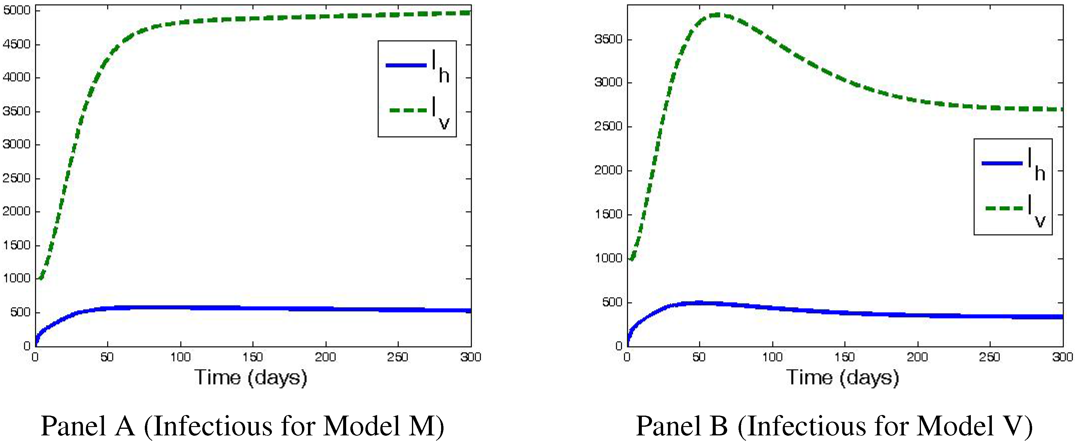
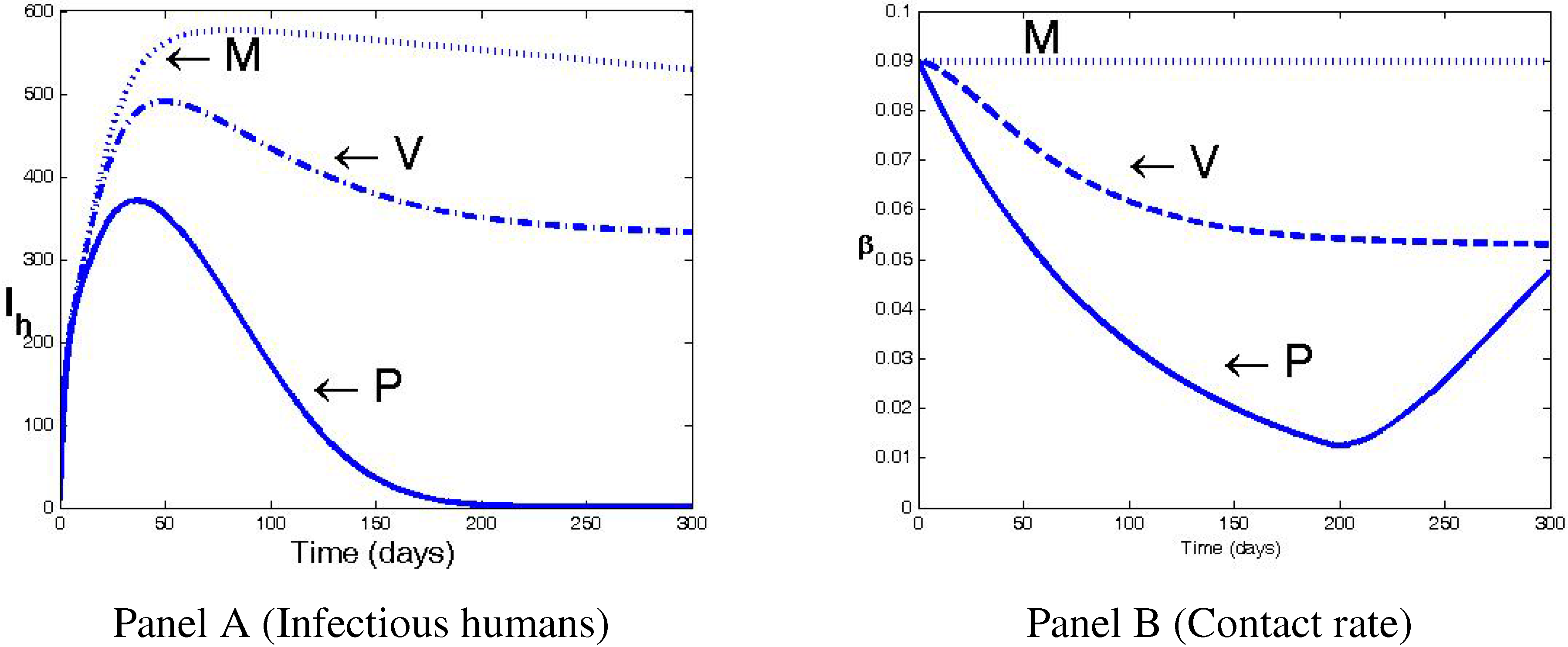
• Case I (Model M): Constant contact rate.

By setting $ϵ=0$ in Equation (7) one gets the structure of classical host–vector models [19,22] (essentially the same happens when Model (1) is considered with b constant, as done in [13]). Assuming $ϵ=0$, and therefore $\beta \left(w\right)={\beta }_{max}\equiv \beta$, we have the following equations, that we call Model M:

$$\begin{array}{cc}{\dot{N}}_h=\hfill & {\Lambda }_h-\mu N_h-\alpha I_h\hfill \\ {\dot{I}}_h=\hfill & p_1\beta \frac{I_v}{N_h}\left(N_h-I_h\right)-(\alpha +\mu +\delta )I_h\hfill \\ {\dot{S}}_v=\hfill & {\Lambda }_v-p_2\beta \frac{I_h}{N_h}{S}_v-\eta S_v\hfill \\ {\dot{I}}_v=\hfill & p_2\beta \frac{I_h}{N_h}{S}_v-\eta I_v,\hfill \end{array}$$

(9)

where $N_h=S_h+I_h$.

• Case II (Model V): Pure voluntary ITNs adoptions.

As already mentioned, the function ψ describes the role played by the state variables and health campaign measures in the goodwill dynamics. In the case of pure voluntary ITNs adoptions, we assume that the individuals will make their choice to adopt or not to adopt ITNs on the basis of the information available on the prevalence of the disease in the community where they live. This constitutes a sort of “social alarm” which we represent as:

$$\psi \left(I_h\left(t\right)\right)=c\left(t\right)\frac{I_h\left(t\right)}{N_h\left(t\right)}$$

(10)

where $c\left(t\right)$ is the information coverage function. We assume that the information is available since $t=0$, so that:

$$c\left(t\right)=\left\{\begin{array}{cc}0\hfill & \mathrm{if}t\le 0\hfill \\ c\hfill & \mathrm{if}t>0\hfill \end{array}\right.$$

(11)

where c is a positive constant.

Assuming $ϵ=1$ and ψ given by Equation (10), from Equations (1), (2) and (8) we get the following Model V:

$$\begin{array}{cc}{\dot{N}}_h=\hfill & {\Lambda }_h-\mu N_h-\alpha I_h\hfill \\ {\dot{I}}_h=\hfill & p_1\beta \left(w\right)\frac{I_v}{N_h}\left(N_h-I_h\right)-(\alpha +\mu +\delta )I_h\hfill \\ {\dot{S}}_v=\hfill & {\Lambda }_v-p_2\beta \left(w\right)\frac{I_h}{N_h}{S}_v-\eta S_v\hfill \\ {\dot{I}}_v=\hfill & p_2\beta \left(w\right)\frac{I_h}{N_h}{S}_v-\eta I_v,\hfill \\ \dot{w}=\hfill & \xi \left(c\frac{I_h}{N_h}-w\right),\hfill \end{array}$$

(12)

where $N_h=S_h+I_h$, $\beta \left(w\right)$ is given by Equation (7) and, for the sake of simplicity, the mosquito killing effect of ITNs has been neglected (i.e., ${\eta }_{bn}=0$ in Equation (4)).

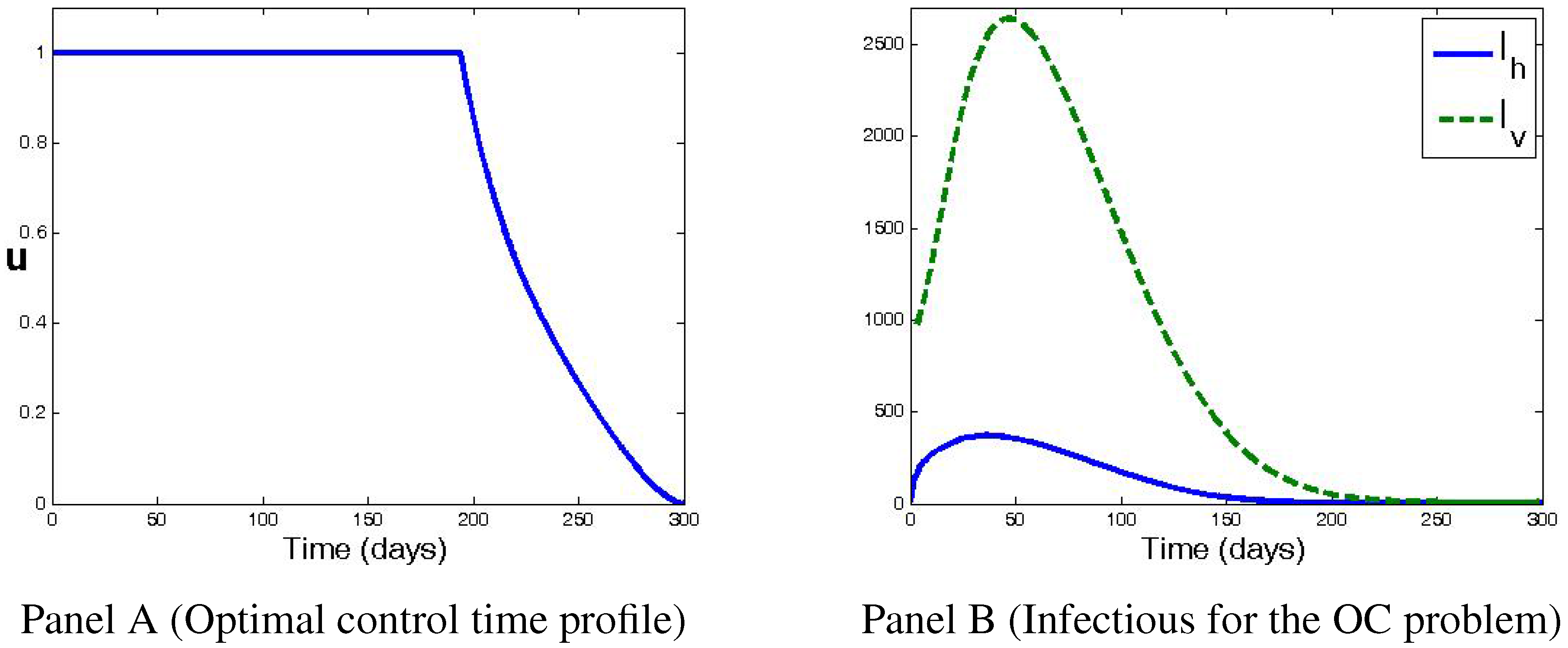
• Case III (Model P): ITNs promotion program.

We represent the message given by the ITNs promotion programs as:

$$\psi \left(u\right(t\left)\right)=c\left(t\right)u\left(t\right),$$

(13)

where $c\left(t\right)$ is given by Equation (11). This assumption means that individuals will adopt or not adopt ITNs only on the basis of the promotion program. In other words, the ‘history’ of the goodwill is affected by (and only by) the campaign effort u.

Assuming $ϵ=1$ and ψ given by Equation (13), from Equations (1), (2) and (8) we get the following system, that we call Model P:

$$\begin{array}{cc}{\dot{N}}_h=\hfill & {\Lambda }_h-\mu N_h-\alpha I_h\hfill \\ {\dot{I}}_h=\hfill & p_1\beta \left(w\right)\frac{I_v}{N_h}\left(N_h-I_h\right)-(\alpha +\mu +\delta )I_h\hfill \\ {\dot{S}}_v=\hfill & {\Lambda }_v-p_2\beta \left(w\right)\frac{I_h}{N_h}{S}_v-\eta S_v\hfill \\ {\dot{I}}_v=\hfill & p_2\beta \left(w\right)\frac{I_h}{N_h}{S}_v-\eta I_v,\hfill \\ \dot{w}=\hfill & \xi \left(u\left(t\right)-w\right),\hfill \end{array}$$

(14)

where $N_h=S_h+I_h$, $\beta \left(w\right)$ is given by Equation (7) and ${\eta }_{bn}=0$ in Equation (4).

3. Optimal ITNs Promotion Campaign

In this section, we will consider Model (14) and look for optimal strategies for implementing ITNs promotion programs. In other words, we aim to determine the optimal effort $u\left(t\right)$ over a finite horizon T for the Case III introduced above. To this aim, we will use a numerically–oriented approach recently proposed in [23] (for background on numerical methods in control theory see [24,25,26]).

As “Optimal” we mean that the campaign target is to minimize the total costs associated with both the disease and the controls. The cost function associated with the disease burden is assumed to be linearly dependent on the size of human infectious compartment, whereas the intervention costs are assumed to increase quadratically with u. This represents the increased cost of large–scale campaign efforts. We stress that a nonlinear cost is particularly appropriate when the effort function refers to an information campaign, since the more the information spreads, the more costly it becomes to reach the remaining unaware individuals. Among the nonlinear representation of intervention costs, the quadratic approximation is the simplest and most widely used (for more details on the choice of quadratic intervention costs when dealing with epidemic models, see, for example, [23,27,28,29,30]).

The objective functional to be minimized is:

$$J\left(u\right)={\int }_0^T\left(A{I}_h+\frac{B}{2}{u}^2\right)dt,$$

(15)

where the control $u\left(t\right)$, $i=1,2$, is a Lebesgue measurable functions such that: $0\le u\left(t\right)\le u_{max}$, for $t\in [0,T]$. In Equation (15), the (positive) constants A and B are weight parameters describing the comparative importance of the two terms in the functional [23]. This optimal control problem may be addressed by the well known Pontryagin’s maximum principle, where the Hamiltonian:

$$H=g(\text{x},u,t)+\sum _{i=1}^5{\lambda }_i\left(t\right){\phi }_i(\text{x},\text{u},t),$$

must be minimized pointwise [23]. Here g is the integrand of the objective functional, $\text{x}$ denotes the state-variables vector, ${\lambda }_i$, $i=1,...,5$, are the adjoints and ${\phi }_i$ denotes the right hand side of the i-th equation of System (14).

A similar optimal control approach for general or specific host–vectors models (but not in the framework of information–dependent models) can be found in [6,31,32,33,34,35].

The optimality system for our problem is derived (see Appendix) and numerically solved by using the so called forward–backward sweep method (FBSM), described in details in [23]. The process begin with an initial guess on the control variable. Then, the state equations are solved simultaneously forward in time, and next the adjoint equations are simultaneously solved backward in time. The control is updated by inserting the new values of states and adjoints into its characterization, and the process is repeated until convergence occurs. As in [23], the solver used for the state and adjoint systems is a Runge-Kutta fourth order procedure. A MATLAB code [38] has been built to perform the simulations.

We remark that the FBSM is an indirect method for solving optimal control problems. It is easy to use and works well for our problem. However, there are several limitations inherent to FBSM use. For example, it may fail to converge depending on parameter values and on the size of time intervals (the convergence of the FBSM has been studied for a basic type of optimal control problem in [36]). Alternative numerical methods for studying optimal control problems similar to the one considered in this paper can be found, e.g., in [23,27] (Chapter 21). See also [37] for an overview on useful numerical software packages.

4. Numerical Simulations and Discussion

In a first simulation, we consider the case of constant contact rate. Therefore we run Model M, given by System (9), with parameter values given in Table 1, except that $\beta =0.09$ and $\eta =0.0524$. This corresponds to Model (1) with ${\beta }_{max}=0.1$, $\eta =1/21$, ${\eta }_{bn}=1/21$, and $b=0.1$. That is to say, the case of a constant ITNs usage proportion of 10%. In [13] it has been shown that in this case the basic reproductive number is greater than the critical value 1 (indeed, it is $R_0=2.37$) and the solutions approach an endemic equilibrium. As in [13], we take initial data $(N_{h0},I_{h0},S_{v0},I_{v0})=(910,10,4000,1000)$. The dynamics of infectious humans and vectors is shown in Figure 1, panel A. It can be seen that the two populations approach a steady state.

Figure 1. Panel A: Dynamics of infectious humans $I_h$ and infectious vector $I_v$ as predicted by Model M (9). The parameter values are given in Table 1, except that $\beta =0.09$ and $\eta =0.0524$. Initial data are $(N_{h0},I_{h0},S_{v0},I_{v0})=(910,10,4000,1000)$. Panel B: Dynamics of $I_h$ and $I_v$ as predicted by Model V (12) with parameter values given in Table 1, except that $\beta =0.09$ and $\eta =0.0524$. Furthermore, $\xi =0.01$, $\gamma =0.01$, $w_{max}=1$. The initial data are $(N_{h0},I_{h0},S_{v0},I_{v0},w_0)=(910,10,4000,1000,0)$.

Figure 1. Panel A: Dynamics of infectious humans $I_h$ and infectious vector $I_v$ as predicted by Model M (9). The parameter values are given in Table 1, except that $\beta =0.09$ and $\eta =0.0524$. Initial data are $(N_{h0},I_{h0},S_{v0},I_{v0})=(910,10,4000,1000)$. Panel B: Dynamics of $I_h$ and $I_v$ as predicted by Model V (12) with parameter values given in Table 1, except that $\beta =0.09$ and $\eta =0.0524$. Furthermore, $\xi =0.01$, $\gamma =0.01$, $w_{max}=1$. The initial data are $(N_{h0},I_{h0},S_{v0},I_{v0},w_0)=(910,10,4000,1000,0)$.

When the pure voluntary ITN adoptions are taken into account, the dynamics is governed by Model V, given by System (12). We run this model with parameter values given in Table 1, except that $\beta =0.09$ and $\eta =0.0524$. Furthermore, $\xi =0.01$, $\gamma =0.01$, $w_{max}=1$, $T=300$. The initial data are $(N_{h0},I_{h0},S_{v0},I_{v0},w_0)=(910,10,4000,1000,0)$. Since $w_0=0$, it follows that the initial contact rate is $\beta =0.09$. The dynamics of infectious humans and vectors, as predicted by Model V, is shown in Figure 1, panel B. At the beginning, the dynamics shown in Panels A and B are essentially the same, since a low level of disease prevalence does not affect the population behavior. However, when the prevalence reaches sufficiently large values, the counter–action by individuals, who begin to use ITNs, results in declining the prevalence level. The infectious populations show a peak around 65 days. However, the maximum value reached by the infectious vectors is much lower than the case of constant contact rate. Finally, the infectious population tends to approach a steady state, as in the previous case. However, the values of the endemic state is now much lower, especially for infectious vectors (there is a reduction of 45%, approximately, at steady state). The difference in infectious humans dynamics, as predicted by Model M and Model V, respectively, can be seen in Figure 2, Panel A.

Figure 2. Predictions by Model M, Model V and by the optimal strategy implemented on Model P. Panel A: Infectious humans. Panel B: contact rate. We use the parameter values given in Table 1, except that $\beta =0.09$ and $\eta =0.0524$. Furthermore, $\xi =0.01$, $\gamma =0.01$. The cost weights are $A=1$, $B=10$. The initial data are $(N_{h0},I_{h0},S_{v0},I_{v0},w_0)=(910,10,4000,1000,0)$.

Figure 2. Predictions by Model M, Model V and by the optimal strategy implemented on Model P. Panel A: Infectious humans. Panel B: contact rate. We use the parameter values given in Table 1, except that $\beta =0.09$ and $\eta =0.0524$. Furthermore, $\xi =0.01$, $\gamma =0.01$. The cost weights are $A=1$, $B=10$. The initial data are $(N_{h0},I_{h0},S_{v0},I_{v0},w_0)=(910,10,4000,1000,0)$.

Figure 3. Panel A: The optimal control profile. Panel B: Dynamics of infectious humans $I_h$ and infectious vector $I_v$ as output of the optimal control problem given by Model P (14) and the minimization of the objective functional (15). The parameter values are those specified in the captions of Figure 1 and Figure 2.

Figure 3. Panel A: The optimal control profile. Panel B: Dynamics of infectious humans $I_h$ and infectious vector $I_v$ as output of the optimal control problem given by Model P (14) and the minimization of the objective functional (15). The parameter values are those specified in the captions of Figure 1 and Figure 2.

Finally, we consider the case of optimal ITNs promotion campaign and its influence on the disease dynamics. In other words, we consider the optimal control problem given by the minimization of the objective functional Equation (15) subject to the differential constraints System (14). We use the parameter values given in Table 1, except that $\beta =0.09$ and $\eta =0.0524$. Furthermore, $\xi =0.01$, $\gamma =0.01$. The cost weights are $A=1$, $B=10$. The initial data are $(N_{h0},I_{h0},S_{v0},I_{v0},w_0)=(910,10,4000,1000,0)$.

In Figure 3 (panel A), it is shown the output time profile corresponding to a 300 days of information campaign. The information effort is at the highest possible value in the first stage of the information campaign. Then, starting from day 200, it switches to zero relatively slowly, with an arc joining the upper and the lower bound of the control.

As shown in Figure 3 (panel B), the result of the optimal strategy is that both the infectious populations (humans and vector) reach an epidemic peak (which is lower than the maximum reached in the previous cases) and decline to zero in the last stage of the information campaign.

In order to make a direct comparison between the output of the three cases considered in Section 2.4, we introduce the quantity:

$$Q={\int }_0^T{I}_h\left(t\right)dt,$$

as a possible measure of the disease burden, and denote this quantity by $Q_M$, $Q_V$ and $Q_P$, according to the case considered. When $T=300$, we may evaluate the reduction of disease burden as:

$$R_1=\frac{Q_M-Q_V}{Q_V}=0.2800;R_2=\frac{Q_V-Q_P}{Q_V}=0.6979;R_3=\frac{Q_M-Q_P}{Q_M}=0.7824;$$

This means that, compared to the case of a constant ITNs usage proportion of 10%, a reduction of 28% of disease burden can be observed when a pure voluntary ITNs adoption, based on the information on prevalence, is considered. On the other hand, compared to this last case, an optimal information campaign strategy, as defined in section 3, produces a reduction of 69.8% of disease burden. This result is even better, 78.2%, when the optimal control results are compared with the output of model M.

It is also interesting to evaluate the effects on the contact rate β of changes in the humans behavior. In Figure 2, panel B, it is shown how a pure voluntary ITNs adoption produces a reduction of β from 0.09 (the constant value considered in model M) to 0.055. It can be also seen how β changes in correspondence to the optimal information campaign strategy. When the campaign efforts begin to decline (around day 200, see Figure 3, panel A) the contact rate is at its minimum ($\beta =0.012$) and begins to increase from there. At the end of the considered time horizon, it is still less than the contact rate predicted by model V.

5. Conclusions

In this work we have focused on mathematical modelling of mosquito-borne disease, where the adoption by individuals of non-pharmaceutical personal protections, like the ITNs, is taken into account. Motivated by the well documented strong influence of behavioral factors in ITNs usage, we have proposed a mathematical approach based on the idea of information–dependent epidemic models.

We have evaluated the effects of feedback produced by the actions taken by individuals as a consequence of: (a) the information available on the status of the disease in the community where they live (i.e., pure voluntary adoptions); or (b) an optimal health-promotion campaign aimed at encouraging people to use ITNs.

We have shown that the results may be very different compared to the output of classical models. For example, in [35] an optimal control problem applied to Model (1–4) has been considered. There, the contact rate given in Equation (3) is reduced by a coefficient $1-\zeta \left(t\right)$, where the function $\zeta \left(t\right)$ is analogous to campaign effort $u\left(t\right)$ used here and must be chosen optimally in the same way (i.e., the costs given in Equation (15) must be minimized). The result is that the control is not able to radically change the dynamics of the system, although it may make faster the decay of infected humans when compared to the case where no controls are used. Instead, with the modeling approach proposed here the controlled system may predict dramatic changes of disease prevalence, as shown in Figure 3, panel A.

Assessing how people react to awareness about their environment’s status is of paramount importance for understanding the epidemic evolution. Indeed, individuals make decisions on the basis of information in their possession and this is a key factor in determining the epidemic fate, especially when the containment measures rely on personal protections to be taken on voluntary basis. Modelling the feedback produced by behavioral changes may drive more realistic dynamics that are not captured by classical approaches. Typical examples are given by the sustained oscillations predicted by information–dependent models in the case of pseudo-rational exemption to vaccination [12,14,16,17] and of information–related changes in contact patterns [12,15,17].

Our results are preliminary. Further developments will include the case of a general memory kernel as well as the case of seasonality (i.e., time–periodic coefficients), which may have a relevant role in the case of mosquito-borne diseases [39,40].

References

1. Global Malaria Programme. World Malaria Report 2014; World Health Organization: Geneva, Switzerland, 2014. [Google Scholar]
2. Wiwanitkit, V. Vaccination against mosquito borne viral infections: Current status. Iran J. Immunol. 2007, 4, 186–196. [Google Scholar] [PubMed]
3. Ramsauer, K.; Schwameis, M.; Firbas, C.; Müllner, M.; Putnak, R.J.; Thomas, S.J.; Desprésd, P.; Tauber, E.; Jilma, B.; Tangy, F. Immunogenicity, safety, and tolerability of a recombinant measles-virus-based chikungunya vaccine: A randomised, double–blind, placebo–controlled, active–comparator, first–in–man trial. Lancet 2015, 15, 519–527. [Google Scholar] [CrossRef]
4. World Health Organization. Malaria Vaccine Development. Available online: http://www.who.int/malaria/areas/vaccine/en/ (accessed on 1 September 2015).
5. Halloran, M.E.; Struchiner, C.J. Modeling transmission dynamics of stage-specific malaria vaccines. Parasitol. Today 1992, 8, 77–85. [Google Scholar] [CrossRef]
6. Prosper, O.; Ruktanonchai, N.; Martcheva, M. Optimal vaccination and bednet maintenance for the control of malaria in a region with naturally acquired immunity. J. Theor. Biol. 2014, 353, 142–156. [Google Scholar] [CrossRef] [PubMed]
7. Lin, F.; Muthuraman, K.; Lawley, M. An optimal control theory approach to non–pharmaceutical interventions. BMC Infect. Dis. 2010, 10, 32–45. [Google Scholar] [CrossRef] [PubMed]
8. Briët, O.J.; Chitnis, N. Effects of changing mosquito host searching behaviour on the cost effectiveness of a mass distribution of long–lasting, insecticidal nets: A modelling study. Malaria J. 2013, 12, 215. [Google Scholar] [CrossRef] [PubMed] [Green Version]
9. Centers for Disease Control and Prevention. Insecticide–Treated Bed Nets. Available online: http://www.cdc.gov/malaria/malaria_worldwide/reduction/itn.html (accessed on 1 September 2015).
10. Lengeler, C. Insecticide–treated bed nets and curtains for preventing malaria. Cochane Database Syst. Rev. 2004. [Google Scholar] [CrossRef]
11. Frey, C.; Traoré, C.; de Allegri, M.; Kouyaté, B.; Müller, O. Compliance of young children with ITN protection in rural Burkina Faso. Malaria J. 2006, 5, 70. [Google Scholar] [CrossRef] [PubMed]
12. Modeling the Interplay Between Human Behavior and the Spread of Infectious Diseases; Manfredi, P.; d’Onofrio, A. (Eds.) Springer: Heidelberg, Germany, 2013.
13. Agusto, F.B.; del Valle, S.Y.; Blayneh, K.W.; Ngonghala, C.N.; Goncalves, M.J.; Li, N.; Zhao, R.; Gong, H. The impact of bed-net use on malaria prevalence. J. Theor. Biol. 2013, 320, 58–65. [Google Scholar] [CrossRef] [PubMed]
14. Buonomo, B.; d’Onofrio, A.; Lacitignola, D. Global stability of an SIR epidemic model with information dependent vaccination. Math. Biosci. 2008, 216, 9–16. [Google Scholar] [CrossRef] [PubMed]
15. Buonomo, B.; d’Onofrio, A.; Lacitignola, D. Globally stable endemicity for infectious diseases with information-related changes in contact patterns. Appl. Math. Lett. 2012, 25, 1056–1060. [Google Scholar] [CrossRef]
16. Buonomo, B.; d’Onofrio, A.; Lacitignola, D. Modeling of pseudo-rational exemption to vaccination for SEIR diseases. J. Math. Anal. Appl. 2013, 404, 385–398. [Google Scholar] [CrossRef]
17. D’Onofrio, A.; Manfredi, P. Information-related changes in contact patterns may trigger oscillations in the endemic prevalence of infectious diseases. J. Theor. Biol. 2009, 256, 473–478. [Google Scholar] [CrossRef] [PubMed]
18. D’Onofrio, A.; Manfredi, P.; Salinelli, E. Vaccinating behaviour, information, and the dynamics of SIR vaccine preventable diseases. Theor. Popul. Biol. 2007, 71, 301–317. [Google Scholar] [CrossRef] [PubMed]
19. Keeling, M.J.; Rohani, P. Modeling Infectious Diseases in Humans and Animals; Princeton University Press: Princeton, NJ, USA, 2007. [Google Scholar]
20. Behncke, H. Optimal control of deterministic epidemics. Optim. Control Appl. Meth. 2000, 21, 269–285. [Google Scholar] [CrossRef]
21. Smith, H. An Introduction to Delay Differential Equations with Applications to the Life Sciences; Springer: Heidelberg, Germany, 2011; Volume 57. [Google Scholar]
22. Macdonald, G. The Epidemiology and Control of Malaria; Oxford University Press: London, UK, 1957. [Google Scholar]
23. Lenhart, S.; Workman, J.T. Optimal Control Applied to Biological Models; Chapman & Hall/CRC Mathematical and Computational Biology Series; Chapman & Hall/CRC: Boca Raton, FL, USA, 2007. [Google Scholar]
24. Isidori, A. Nonlinear Control Systems; Springer: Berlin, Germany, 1989. [Google Scholar]
25. Sontag, E.D. Mathematical Control Theory, 2nd ed.; Springer: Berlin; Heidelberg, Germany, 1998. [Google Scholar]
26. Nonlinear Controllability and Optimal Control; Sussmann, H.J. (Ed.) Dekker: New York, NY, USA, 1990.
27. Anita, S.; Arnautu, V.; Capasso, V. An Introduction to Optimal Control Problems in Life Sciences and Economics; Birkhäuser: Boston, MA, USA, 2010. [Google Scholar]
28. Buonomo, B. A simple analysis of vaccination strategies for rubella. Math. Biosci. Eng. 2011, 8, 677–687. [Google Scholar] [CrossRef] [PubMed]
29. Buonomo, B. On the optimal vaccination strategies for horizontally and vertically transmitted infectious diseases. J. Biol. Sys. 2011, 19, 263–279. [Google Scholar] [CrossRef]
30. Hocking, L.M. Optimal control. In An Introduction to the Theory with Applications; Oxford University Press: Oxford, UK, 1991. [Google Scholar]
31. Ozair, M.; Lashari, A.A.; Jung, I.H.; Okosun, K.O. Stability analysis and optimal control of a vector-borne disease with nonlinear incidence. Discrete Dyn. Nat. Soc. 2012. [Google Scholar] [CrossRef]
32. Aldila, D.; Götz, T.; Soewono, E. An optimal control problem arising from a dengue disease transmission model. Math. Biosci. 2013, 242, 9–16. [Google Scholar] [CrossRef] [PubMed]
33. Kong, Q.; Qiu, Z.; Sang, Z.; Zou, Y. Optimal control of a vector-host epidemics model. Math. Control Rel. Fields 2011, 1, 493–508. [Google Scholar] [CrossRef]
34. Agusto, F.B.; Marcus, N.; Okosun, K.O. Application of optimal control to the epidemiology of malaria. Electron. J. Diff. Eq. 2012, 2012, 1–22. [Google Scholar]
35. Silva, C.J.; Torres, D.F.M. An optimal control approach to malaria prevention via insecticide-treated nets. Conf. Pap. Math. 2013. [Google Scholar] [CrossRef]
36. McAsey, M.; Mou, L.; Han, W. Convergence of the forward-backward sweep method in optimal control. Comput. Opt. Appl. 2012, 53, 207–226. [Google Scholar] [CrossRef]
37. Rodrigues, H.S.; Monteiro, M.T.T.; Torres, D.F.M. Optimal control and numerical software: An overview. In Systems Theory: Perspectives, Applications and Developments; Miranda, F., Ed.; Nova Science Publishers: New York, NY, USA, 2014. [Google Scholar]
38. MATLAB Release 2010b; The MathWorks, Inc.: Natick, MA, USA, 2010.
39. Chitnis, N.; Hardy, D.; Smith, T. A Periodically-forced mathematical model for the seasonal dynamics of malaria in mosquitoes. Bull. Math. Biol. 2012, 74, 1098–1124. [Google Scholar] [CrossRef] [PubMed]
40. Rodrigues, H.S.; Monteiro, M.T.T.; Torres, D.F.M. Seasonality effects on dengue: Basic reproduction number, sensitivity analysis and optimal control. Math. Meth. Appl. Sci. 2015, in press. [Google Scholar]
41. Grass, D.; Caulkins, J.P.; Feichtinger, G.; Tragler, G.; Behrens, D.A. Optimal Control of Nonlinear Processes, with Applications in Drugs, Corruption, and Terror; Springer: Berlin, Germany, 2008. [Google Scholar]