
From Cayley-Dickson Algebras to Combinatorial Grassmannians


1
Astronomical Institute, Slovak Academy of Sciences, Tatranská Lomnica 05960, Slovak Republic
2
IRTES/UTBM, Université de Bourgogne Franche-Comté, Belfort Cedex 90010, France
3
J. Heyrovský Institute of Physical Chemistry, v. v. i., Academy of Sciences of the Czech Republic, Dolejškova 3, Prague 18223, Czech Republic
*
Author to whom correspondence should be addressed.
Mathematics 2015, 3(4), 1192-1221; https://doi.org/10.3390/math3041192
Submission received: 23 August 2015
/
Revised: 26 November 2015
/
Accepted: 30 November 2015
/
Published: 4 December 2015
Abstract
:Given a -dimensional Cayley-Dickson algebra, where , we first observe that the multiplication table of its imaginary units , , is encoded in the properties of the projective space PG if these imaginary units are regarded as points and distinguished triads of them , and , as lines. This projective space is seen to feature two distinct kinds of lines according as or . Consequently, it also exhibits (at least two) different types of points in dependence on how many lines of either kind pass through each of them. In order to account for such partition of the PG, the concept of Veldkamp space of a finite point-line incidence structure is employed. The corresponding point-line incidence structure is found to be a specific binomial configuration ; in particular, (octonions) is isomorphic to the Pasch -configuration, (sedenions) is the famous Desargues -configuration, (32-nions) coincides with the Cayley-Salmon -configuration found in the well-known Pascal mystic hexagram and (64-nions) is identical with a particular -configuration that can be viewed as four triangles in perspective from a line where the points of perspectivity of six pairs of them form a Pasch configuration. Finally, a brief examination of the structure of generic leads to a conjecture that is isomorphic to a combinatorial Grassmannian of type .
1. Introduction
As it is well known (see, for example, [1,2]), the Cayley-Dickson algebras represent a nested sequence of -dimensional (in general non-associative) -algebras with , where and where for any the set comprises all ordered pairs of elements from with conjugation defined by:
and multiplication by:
Every finite-dimensional algebra (see, for example, [2]) is defined by the multiplication rule of its basis. The basis elements (or units) of , being the real basis element (identity), can be chosen in various ways. Our preference is the canonical basis:
where, by abuse of notation (see, for example, [3]), the same symbols are also used for the basis elements of . This is because the paper essentially focuses on multiplication properties of basis elements and the canonical basis seems to display most naturally the inherent symmetry of this operation. For, in addition to revealing the nature of the Cayley-Dickson recursive process, it also implies that for both a and b being non-zero we have where the symbol “⊕” denotes “exclusive or” of the binary representations of a and b (see, for example, [4]). From the above expressions and Equation (1) and Equation (2) one can readily find the product of any two distinct units of if the multiplication properties of those of are given. Such products are usually expressed/presented in a tabular form, and we shall also follow this tradition here. All the multiplication tables we made use of were computed for us by Jörg Arndt; the computer program is named cayley-dickson-demo.cc and is freely available from his web-site [5].
Employing such a multiplication table of , , it can be verified that the imaginaries , , form distinguished sets each of which comprises three different units that satisfy the equation:
and where each unit is found to belong to such sets. (Although these properties will explicitly be illustrated only for the cases , due to the nested structure of the algebras they must be exhibited by any other higher-dimensional .). Regarding the imaginaries as points and their distinguished triples as lines, one gets a point-line incidence geometry where every line has three points and through each point there pass lines and which is isomorphic to PG, the -dimensional projective space over the smallest Galois field (see also [6] for and [7] for ). Let us assume, without loss of generality, that the elements in any distinguished triple of are ordered in such a way that . Then, for , we can naturally speak about two different kinds of triples and, hence, two distinct kinds of lines of the associated -nionic PG, according as or ; in what follows a line of the former kind will be called ordinary and that of the latter kind defective. This stratification of the line-set of the PG induces a similar partition of the point-set of the latter space into several types, where a point of a given type is characterized by the same number of lines of either kind that pass through it.
Obviously, if our projective space PG is regarded as an abstract geometry per se, every point and/or every line in it has the same footing. So, to account for the above-described “refinement” of the structure of our -nionic PG, it turns out to be necessary to find a representation of this space where each point/line is ascribed a certain “internal” structure, which at first sight may seem to be quite a challenging task. To tackle this task successfully, we need to introduce a few ideas from the realm of finite geometry.
We start with a finite point-line incidence structure where and are finite sets of points and lines and where incidence is a binary relation indicating which point-line pairs are incident (see, for example, [8]). Here, we shall only be concerned with specific point-line incidence structures called configurations [9]. A -configuration is a where: (1) and ; (2) every line has k points and every point is on r lines; and (3) two distinct lines intersect in at most one point and every two distinct points are joined by at most one line; a configuration where and is called symmetric (or balanced), and usually denoted as a -configuration. A -configuration with and is called a configuration. Next, we define a geometric hyperplane of , which is a proper subset of such that a line from either lies fully in the subset, or shares with it only one point. If possesses geometric hyperplanes, then one can define the Veldkamp space of , , as follows [10]: (i) a point of is a geometric hyperplane of and (ii) a line of is the collection of all geometric hyperplanes H of such that or , where and are distinct geometric hyperplanes. If each line of has three points and “behaves well”, a line of is also of size three and can equivalently be defined as , where the symbol Δ stands for the symmetric difference of the two geometric hyperplanes and an overbar denotes the complement of the object indicated. From its definition it is obvious that is well suited for our needs because its points, being themselves sets of points, have different “internal” structure and so, in general, they can no longer be on the same par; clearly, the same applies to the lines . Our task thus basically boils down to finding such whose is isomorphic to PG and completely reproduces its -nionic fine structure. This will be carried out in great detail for the first four non-trivial cases, , which, when combined with the two trivial cases (), will provide us with sufficient amount of information to guess a general pattern.
The paper is organized as follows. In Section 2 it is shown that (octonions) is isomorphic to the Pasch -configuration, which plays a key role in classifying Steiner triple systems. In Section 3 one demonstrates that (sedenions) is nothing but the famous Desargues -configuration. In Section 4 our (32-nions) is shown to be identical with the Cayley-Salmon -configuration found in the well-known Pascal mystic hexagram. In Section 5 we find that corresponds to a particular -configuration encompassing seven distinct copies of the Cayley-Salmon -configuration as geometric hyperplanes. In Section 6 some rudimentary properties of the generic -configuration are outlined and its isomorphism to a combinatorial Grassmannian of type is conjectured. Finally, Section 7 is reserved for concluding remarks.
2. Octonions and the Pasch -Configuration
From the nesting property of the Cayley-Dickson construction of it is obvious that the smallest non-trivial case to be addressed is , the algebra of octonions, whose multiplication table is presented in Table 1.

Table 1.
The multiplication table of the imaginary unit octonions , . For the sake of simplicity, in what follows we shall employ a short-hand notation ; likewise for the real unit . There are also delineated multiplication tables corresponding to the distinguished nested sequence of sub-algebras of complex numbers (, the upper left corner) and quaternions (, the upper left square).
| * | 1 | 2 | 3 | 4 | 5 | 6 | 7 |
|---|---|---|---|---|---|---|---|
| 1 | −0 | −3 | +2 | −5 | +4 | +7 | −6 |
| 2 | +3 | −0 | −1 | −6 | −7 | +4 | +5 |
| 3 | −2 | +1 | −0 | −7 | +6 | −5 | +4 |
| 4 | +5 | +6 | +7 | −0 | −1 | −2 | −3 |
| 5 | −4 | +7 | −6 | +1 | −0 | +3 | −2 |
| 6 | −7 | −4 | +5 | +2 | −3 | −0 | +1 |
| 7 | +6 | −5 | −4 | +3 | +2 | −1 | −0 |
The above-given multiplication table implies the existence of the following seven distinguished trios of imaginary units:
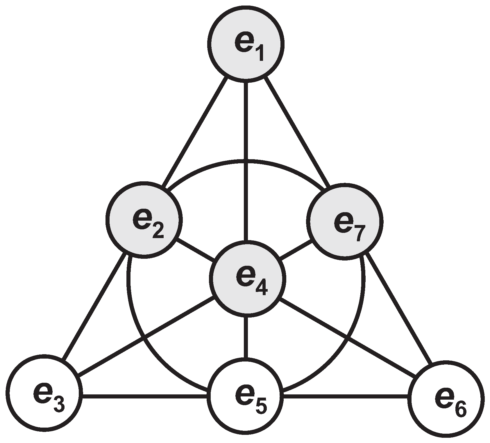
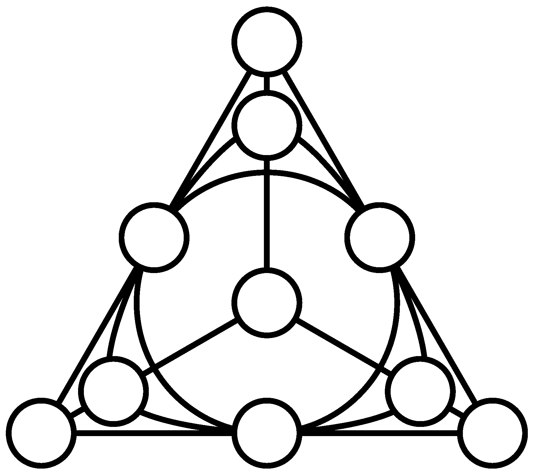
Regarding the seven imaginary units as points and the seven distinguished triples of them as lines, we obtain a point-line incidence structure where each line has three points and, dually, each point is on three lines, and which is isomorphic to the smallest projective plane PG, often called the Fano plane, depicted in Figure 1.
It is then readily seen that we have six ordinary lines, namely:
and only single defective one, that is:
Similarly, our octonionic PG features two distinct types of points. A type-one point is such that two lines passing through it are ordinary, the remaining one being defective; such a point lies in the set:
A type-two point is such that every line passing through it is ordinary; such a point belongs to the set:
which is highlighted by gray color in Figure 1.
Figure 1.
An illustration of the structure of PG, the Fano plane, that provides the multiplication law for octonions (see, e.g., [6]). The points of the plane are seven small circles. The lines are represented by triples of circles located on the sides of the triangle, on its altitudes, and by the triple lying on the big circle. The three imaginaries lying on the same line satisfy Equation (3).

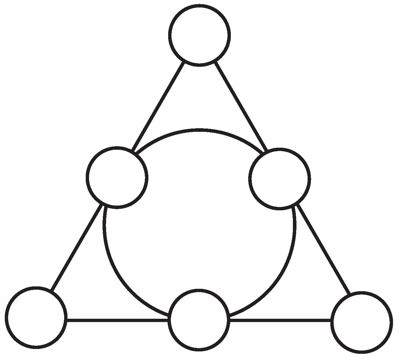
A configuration whose Veldkamp space reproduces the above-described partitions of points and lines of PG is, as we will soon see, nothing but the well-known Pasch -configuration, . This configuration, which plays a very important role in classifying Steiner triple systems (see, for example, [11]), is depicted in Figure 2 in a form showing an automorphism of order three; it also lives in the Fano plane and, as it is readily seen by comparing Figure 1 and Figure 2, it can be obtained from the latter by removal of any of its seven points and all the three lines passing through it.
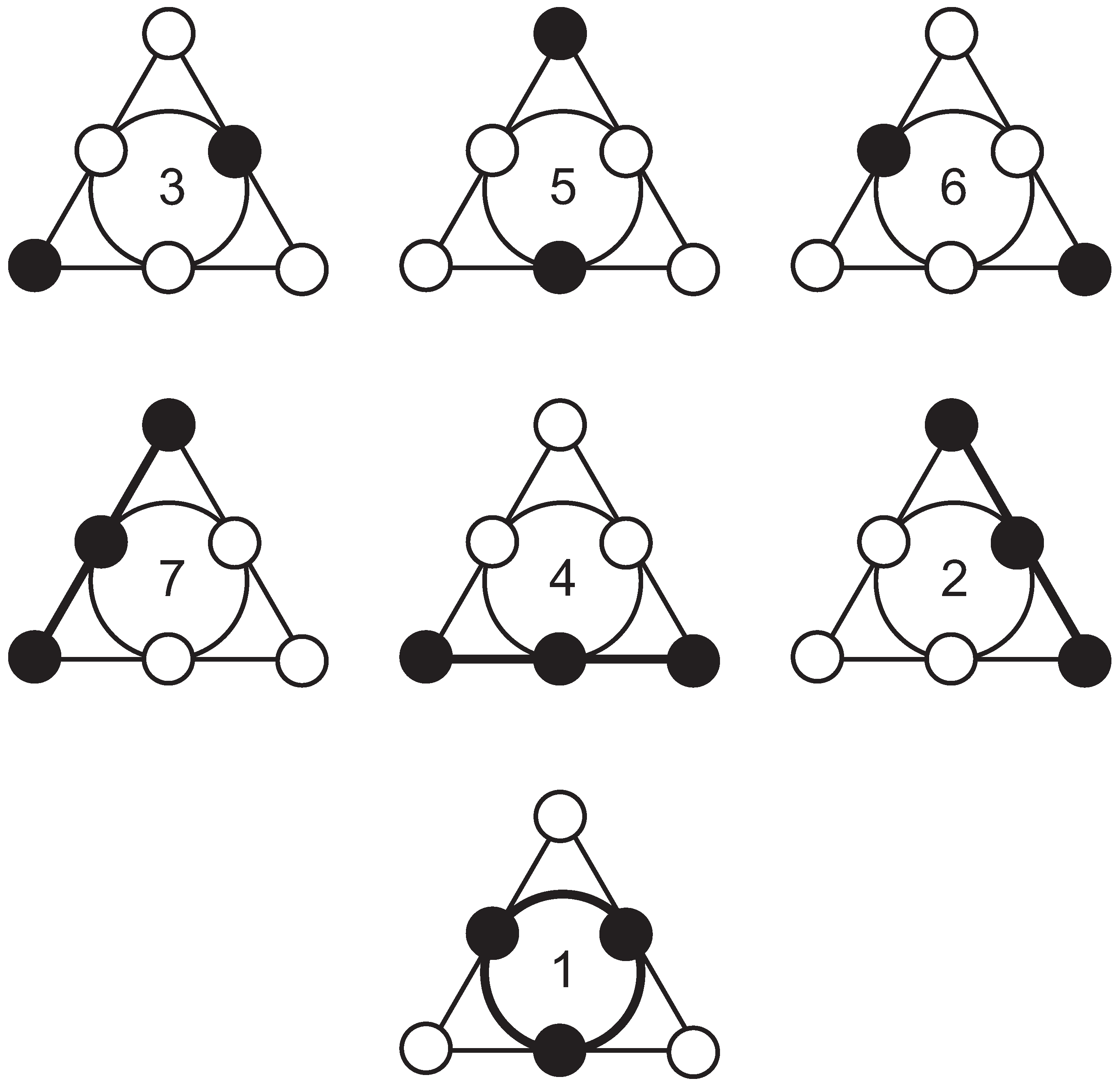
In order to see that PG we shall first show, using our diagrammatical representation of , all seven geometric hyperplanes of —Figure 3. We see that they are indeed of two different forms, of cardinality three and four. A member of the former set comprises two points at maximum distance from each other. Such geometric hyperplane corresponds to a type-one (or α-) point of PG. A member of the latter set features three points on a common line; such a geometric hyperplane of corresponds to a type-two (or β-) point of our PG. The seven lines of are illustrated in a compact diagrammatic form in Figure 4; as it is easily discernible, each of the six ordinary lines is of the form , whilst the remaining defective one has the shape.
Figure 2.
An illustrative portrayal of the Pasch configuration: circles stand for its points, whereas its lines are represented by triples of points on common straight segments (three) and the triple lying on a big circle.
Figure 2.
An illustrative portrayal of the Pasch configuration: circles stand for its points, whereas its lines are represented by triples of points on common straight segments (three) and the triple lying on a big circle.

Figure 3.
The seven geometric hyperplanes of the Pasch configuration. The hyperplanes are labelled by imaginary units of octonions in such a way that the seven lines of the Veldkamp space of the Pasch configuration are identical with the seven distinguished triples of units, that is with the seven lines of the PG shown in Figure 1.

Figure 4.
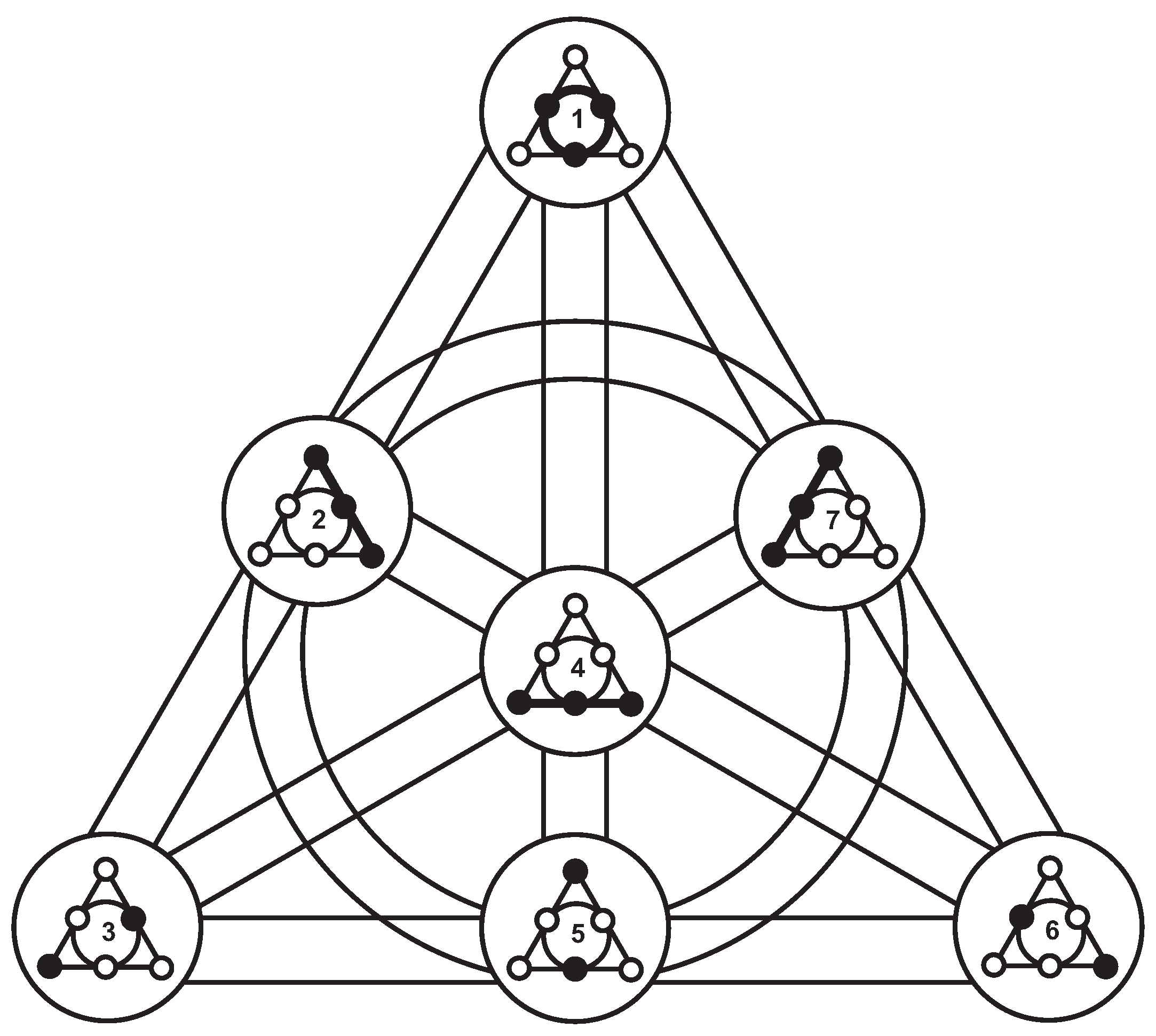
A unified view of the seven Veldkamp lines of the Pasch configuration. The reader can readily verify that for any three geometric hyperplanes lying on a given line of the Fano plane, one is the complement of the symmetric difference of the other two.
Figure 4.
A unified view of the seven Veldkamp lines of the Pasch configuration. The reader can readily verify that for any three geometric hyperplanes lying on a given line of the Fano plane, one is the complement of the symmetric difference of the other two.

3. Sedenions and the Desargues -Configuration
Our next focus is on , the sedenions, whose basic multiplication properties are summarized in Table 2.
An inspection of this table yields as many as 35 distinguished triples, namely:
Regarding the 15 imaginary units as points and the 35 distinguished trios of them as lines, we obtain a point-line incidence structure where each line has three points and each point is on seven lines, and which is isomorphic to PG, the smallest projective space—as depicted in Figure 5. The latter figure employs a diagrammatical model of PG built, after Polster [12], around the pentagonal model of the generalized quadrangle of type GQ whose 15 lines are illustrated by triples of points lying on black line-segments (10 of them) and/or black arcs of circles (5). The remaining 20 lines of PG comprise four distinct orbits: the yellow, red, blue and green one consisting, respectively, of the yellow (), red (), blue () and green () line and other four lines we get from each by rotation through 72 degrees around the center of the pentagon.
Table 2.
The multiplication table of the imaginary unit sedenions , . As in the previous section, we shall employ a short-hand notation ; likewise for the real unit . There are also shown multiplication tables corresponding to the distinguished nested sequence of sub-algebras starting with complex numbers (), quaternions () and octonions ().
| * | 1 | 2 | 3 | 4 | 5 | 6 | 7 | 8 | 9 | 10 | 11 | 12 | 13 | 14 | 15 |
|---|---|---|---|---|---|---|---|---|---|---|---|---|---|---|---|
| 1 | −0 | −3 | +2 | −5 | +4 | +7 | −6 | −9 | +8 | +11 | −10 | +13 | −12 | −15 | +14 |
| 2 | +3 | −0 | −1 | −6 | −7 | +4 | +5 | −10 | −11 | +8 | +9 | +14 | +15 | −12 | −13 |
| 3 | −2 | +1 | −0 | −7 | +6 | −5 | +4 | −11 | +10 | −9 | +8 | +15 | −14 | +13 | −12 |
| 4 | +5 | +6 | +7 | −0 | −1 | −2 | −3 | −12 | −13 | −14 | −15 | +8 | +9 | +10 | +11 |
| 5 | −4 | +7 | −6 | +1 | −0 | +3 | −2 | −13 | +12 | −15 | +14 | −9 | +8 | −11 | +10 |
| 6 | −7 | −4 | +5 | +2 | −3 | −0 | +1 | −14 | +15 | +12 | −13 | −10 | +11 | +8 | −9 |
| 7 | +6 | −5 | −4 | +3 | +2 | −1 | −0 | −15 | −14 | +13 | +12 | −11 | −10 | +9 | +8 |
| 8 | +9 | +10 | +11 | +12 | +13 | +14 | +15 | −0 | −1 | −2 | −3 | −4 | −5 | −6 | −7 |
| 9 | −8 | +11 | −10 | +13 | −12 | −15 | +14 | +1 | −0 | +3 | −2 | +5 | −4 | −7 | +6 |
| 10 | −11 | −8 | +9 | +14 | +15 | −12 | −13 | +2 | −3 | −0 | +1 | +6 | +7 | −4 | −5 |
| 11 | +10 | −9 | −8 | +15 | −14 | +13 | −12 | +3 | +2 | −1 | −0 | +7 | −6 | +5 | −4 |
| 12 | −13 | −14 | −15 | −8 | +9 | +10 | +11 | +4 | −5 | −6 | −7 | −0 | +1 | +2 | +3 |
| 13 | +12 | −15 | +14 | −9 | −8 | −11 | +10 | +5 | +4 | −7 | +6 | −1 | −0 | −3 | +2 |
| 14 | +15 | +12 | −13 | −10 | +11 | −8 | −9 | +6 | +7 | +4 | −5 | −2 | +3 | −0 | −1 |
| 15 | −14 | +13 | +12 | −11 | −10 | +9 | −8 | +7 | −6 | +5 | +4 | −3 | −2 | +1 | −0 |
Figure 5.
An illustration of the structure of PG that provides the multiplication law for sedenions. As in the previous case, the three imaginaries lying on the same line are such that the product of two of them yields the third one, sign disregarded.
Figure 5.
An illustration of the structure of PG that provides the multiplication law for sedenions. As in the previous case, the three imaginaries lying on the same line are such that the product of two of them yields the third one, sign disregarded.
It is not difficult to verify that we have 25 ordinary lines, namely:
and 10 defective ones, namely:
Similarly, our sedenionic PG features two distinct types of points. A type-one point is such that four lines passing through it are ordinary, the remaining three being defective; such a point lies in the set :
A type-two point is such that every line passing through it is ordinary; such a point belongs to the set:
being illustrated by gray shading in Figure 5. We see that all defective lines are of the same form, namely . The 25 ordinary lines split into two distinct families. Ten of them are of the form , namely:
and the remaining 15 are of the form , namely:
A configuration whose Veldkamp space reproduces the above-described partitions of points and lines of PG is, as demonstrated below, the famous Desargues -configuration, , which is one of the most prominent point-line incidence structures (see, for example, [13]). Up to isomorphism, there exist altogether 10 -configurations. The Desargues configuration is, unlike the others, flag-transitive and the only one where for each of its points the three points that are not collinear with it lie on a line. This configuration, depicted in Figure 6 in a form showing its automorphism of order three, also lives in our sedenionic PG; here, its points are the 10 α-points and its lines are all the defective lines. In order to see that PG we shall first introduce, using our diagrammatical representation of , all 15 geometric hyperplanes of —Figure 7. We see that they are indeed of two different forms, and of required cardinality ten and five. A member of the former set comprises a point and three points not collinear with it. Such geometric hyperplane corresponds to a type-one (or α-) point of PG. A member of the latter set features six points located on four lines, with two lines per each point; this is nothing but the Pasch configuration we introduced in the previous section. Such a geometric hyperplane of corresponds to a type-two (or β-) point of our PG. It is also a straightforward task to verify that is endowed with 35 lines splitting into the required three families; those that correspond to defective lines of our sedenionic PG are shown in Figure 8, while those that correspond to ordinary lines are depicted in Figure 9 (of type ) and Figure 10 (of type ). Figure 11 offers a “condensed” view of the isomorphism PG.
Figure 6.
An illustrative portrayal of the Desargues configuration, built around the model of the Pasch configuration shown in Figure 2: circles stand for its points, whereas its lines are represented by triples of points on common straight segments (six), arcs of circles (three) and a big circle.
Figure 6.
An illustrative portrayal of the Desargues configuration, built around the model of the Pasch configuration shown in Figure 2: circles stand for its points, whereas its lines are represented by triples of points on common straight segments (six), arcs of circles (three) and a big circle.

We shall finalize this section by pointing out that the existence of two different kinds of geometric hyperplanes of the Desargues configuration is closely connected with two well-known views of this configuration. The first one is as a pair of triangles that are in perspective from both a point and a line (Desargues’ theorem), the point and the line forming a geometric hyperplane. The other view is as the incidence sum of a complete quadrangle (i.e., a -configuration) and a Pasch -configuration [18].
Figure 7.
The 15 geometric hyperplanes of the Desargues configuration. The hyperplanes are labelled by imaginary units of sedenions in such a way that—as we shall verify in the next three figures—the 35 lines of the Veldkamp space of the Desargues configuration are identical with the 35 distinguished triples of units, that is with the 35 lines of the PG shown in Figure 5.
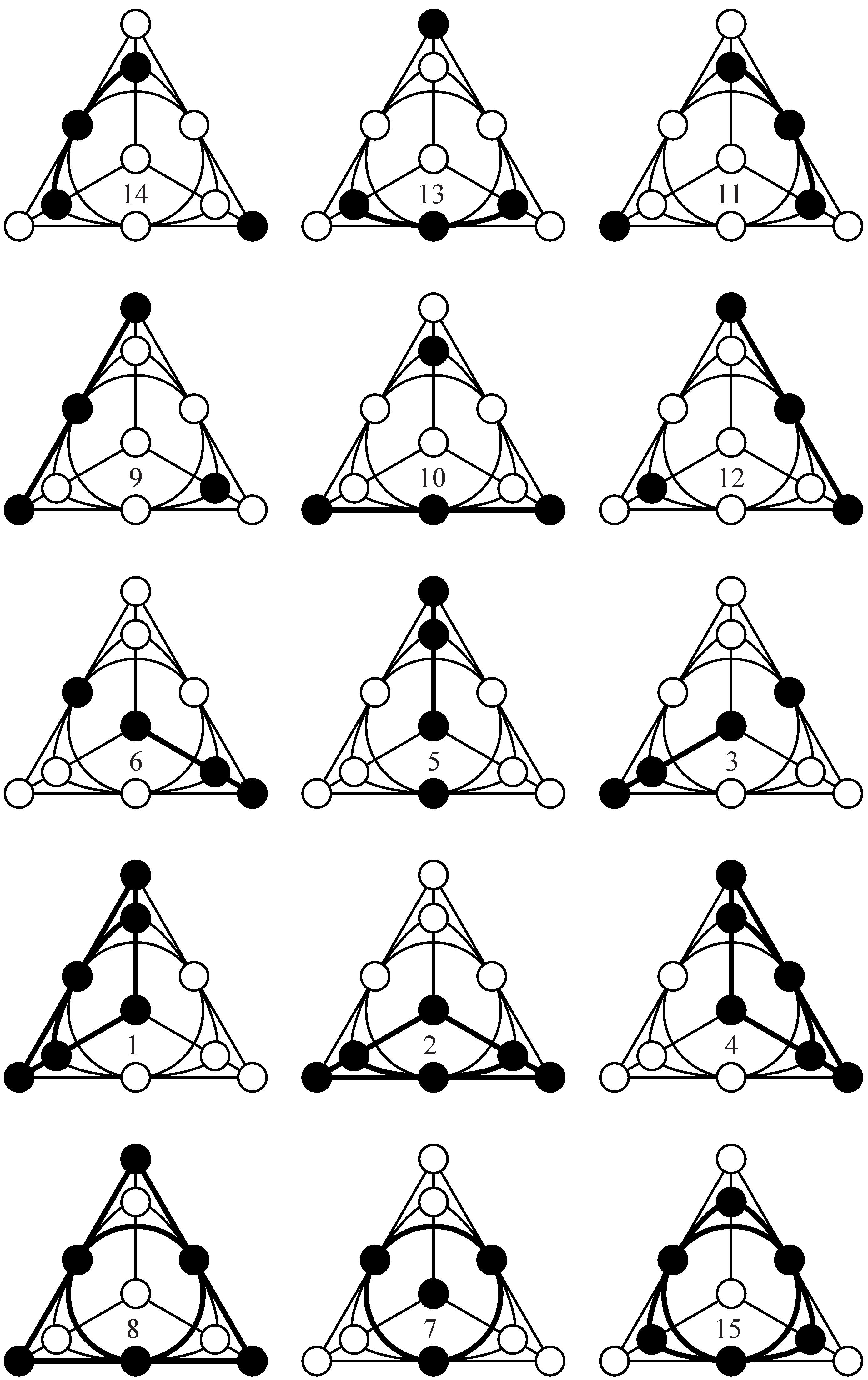
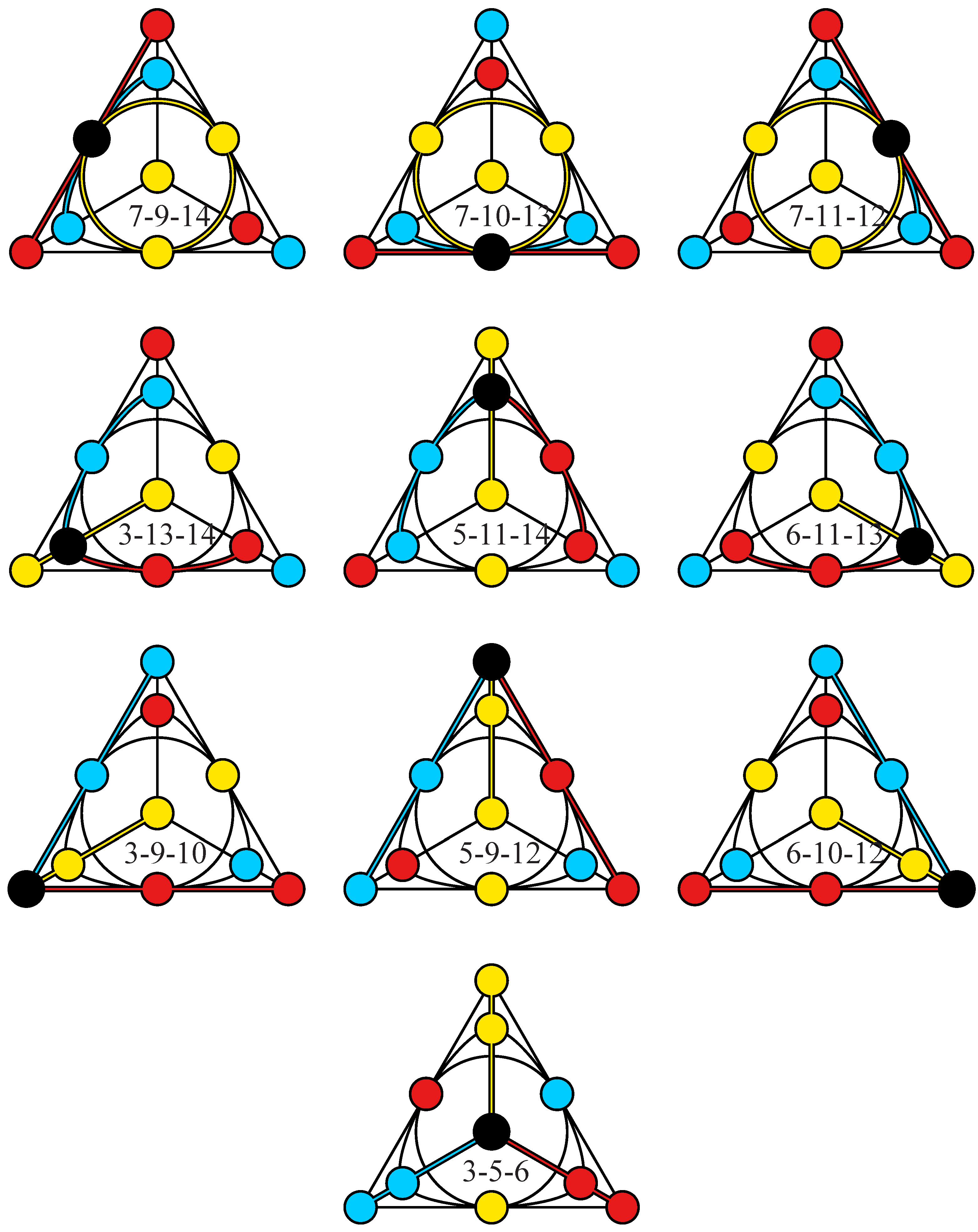
Figure 8.
The 10 Veldkamp lines of the Desargues configuration that represent the 10 defective lines of the sedenionic PG. Here, as well as in the next two figures, the three geometric hyperplanes comprising a given Veldkamp line are distinguished by different colors, with their common elements (here just a single point) being colored black. For each Veldkamp line we also explicitly indicate its composition.

Figure 9.
The 10 Veldkamp lines of the Desargues configuration that represent the 10 ordinary lines of the sedenionic PG of type .
Figure 9.
The 10 Veldkamp lines of the Desargues configuration that represent the 10 ordinary lines of the sedenionic PG of type .

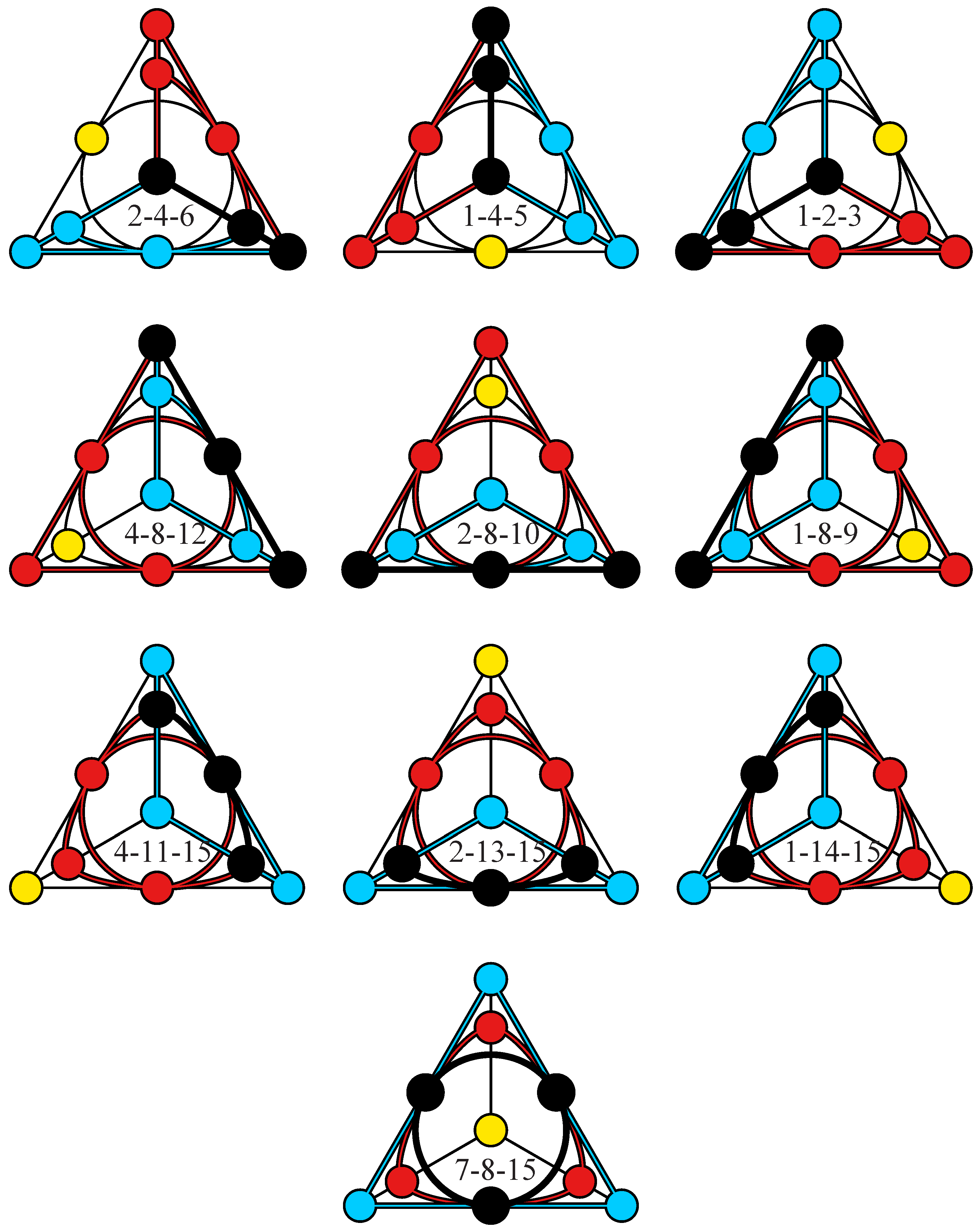
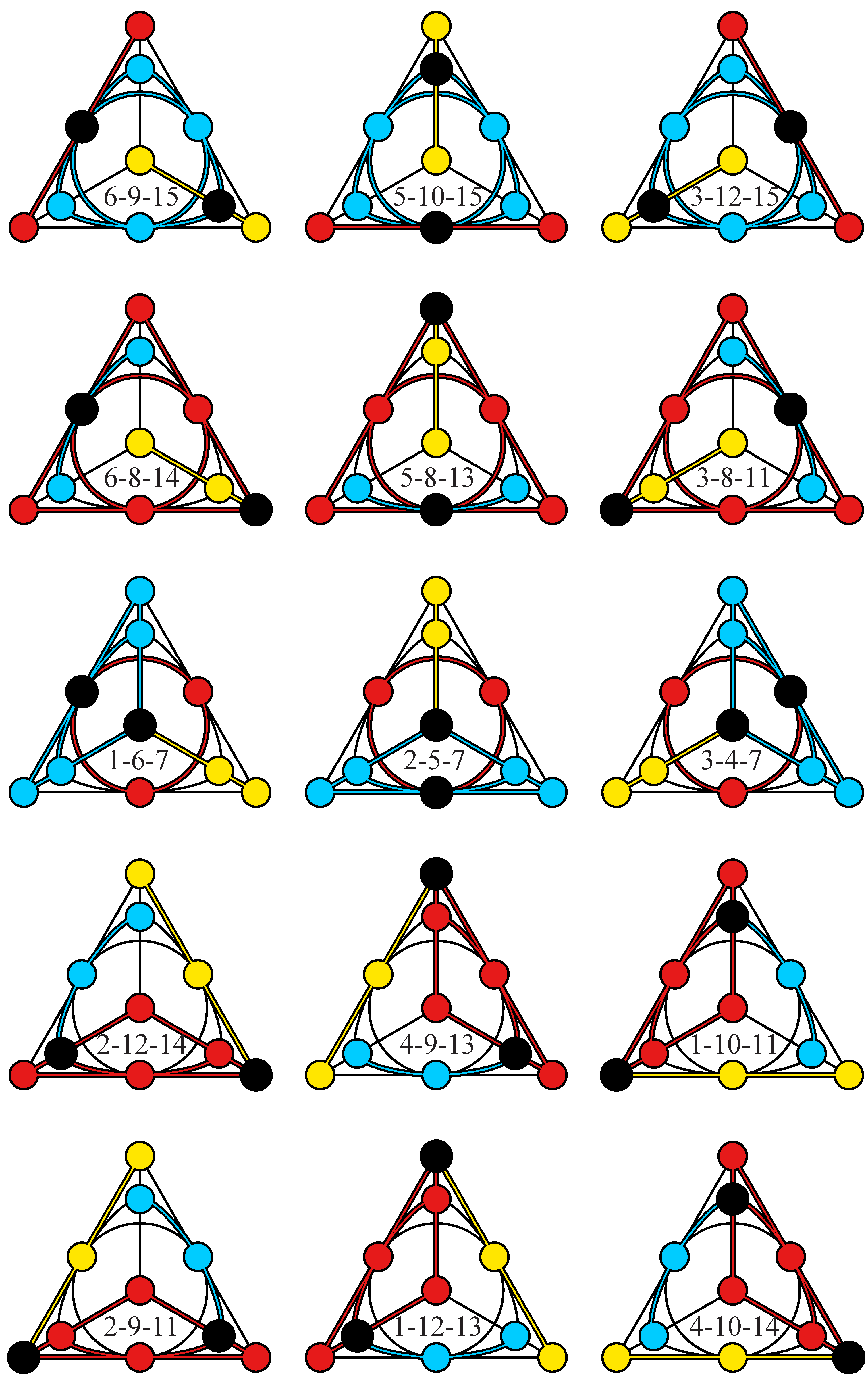
Figure 10.
The 15 Veldkamp lines of the Desargues configuration that represent the 15 ordinary lines of the sedenionic PG of type .
Figure 10.
The 15 Veldkamp lines of the Desargues configuration that represent the 15 ordinary lines of the sedenionic PG of type .

Figure 11.
A compact graphical view of illustrating the bijection between 15 imaginary unit sedenions and 15 geometric hyperplanes of the Desargues configuration, as well as between 35 distinguished triples of units and 35 Veldkamp lines of the Desargues configuration.
Figure 11.
A compact graphical view of illustrating the bijection between 15 imaginary unit sedenions and 15 geometric hyperplanes of the Desargues configuration, as well as between 35 distinguished triples of units and 35 Veldkamp lines of the Desargues configuration.
4. 32-Nions and the Cayley-Salmon -Configuration
Our next case is , or the 32-nions, whose multiplication properties are encoded in Table 3.
From this table we infer the existence of 155 distinguished triples of imaginary units. Regarding the 31 imaginary units of as points and the 155 distinguished triples of them as lines, we obtain a point-line incidence structure where each line has three points and each point is on 15 lines, and which is isomorphic to PG. We next find that 65 lines of this space are defective and 90 ordinary. However, unlike the preceding two cases, there are three different types of points in our 32-nionic PG: 10 α-points,
each of which is on nine defective and six ordinary lines; 15 β-points,
each of which is on seven defective and eight ordinary lines; and six γ-points,
each of them being on 15 ordinary (and, hence, on zero defective) lines. This stratification of the point-set of PG leads, in turn, to two different kinds of defective lines and three distinct kinds of ordinary lines. Concerning the former, there are 45 of them of type , namely:
and 20 of type , namely:
As per the latter, one finds 15 of them of type , namely:
60 of type , namely:
and, finally, 15 of type , namely:
Table 3.
The multiplication table—for better readability split into two parts—of the imaginary unit 32-nions , , in short-hand notation (and ).
| * | 1 | 2 | 3 | 4 | 5 | 6 | 7 | 8 | 9 | 10 | 11 | 12 | 13 | 14 | 15 | |
|---|---|---|---|---|---|---|---|---|---|---|---|---|---|---|---|---|
| 1 | −0 | −3 | +2 | −5 | +4 | +7 | −6 | −9 | +8 | +11 | −10 | +13 | −12 | −15 | +14 | |
| 2 | +3 | −0 | −1 | −6 | −7 | +4 | +5 | −10 | −11 | +8 | +9 | +14 | +15 | −12 | −13 | |
| 3 | −2 | +1 | −0 | −7 | +6 | −5 | +4 | −11 | +10 | −9 | +8 | +15 | −14 | +13 | −12 | |
| 4 | +5 | +6 | +7 | −0 | −1 | −2 | −3 | −12 | −13 | −14 | −15 | +8 | +9 | +10 | +11 | |
| 5 | −4 | +7 | −6 | +1 | −0 | +3 | −2 | −13 | +12 | −15 | +14 | −9 | +8 | −11 | +10 | |
| 6 | −7 | −4 | +5 | +2 | −3 | −0 | +1 | −14 | +15 | +12 | −13 | −10 | +11 | +8 | −9 | |
| 7 | +6 | −5 | −4 | +3 | +2 | −1 | −0 | −15 | −14 | +13 | +12 | −11 | −10 | +9 | +8 | |
| 8 | +9 | +10 | +11 | +12 | +13 | +14 | +15 | −0 | −1 | −2 | −3 | −4 | −5 | −6 | −7 | |
| 9 | −8 | +11 | −10 | +13 | −12 | −15 | +14 | +1 | −0 | +3 | −2 | +5 | −4 | −7 | +6 | |
| 10 | −11 | −8 | +9 | +14 | +15 | −12 | −13 | +2 | −3 | −0 | +1 | +6 | +7 | −4 | −5 | |
| 11 | +10 | −9 | −8 | +15 | −14 | +13 | −12 | +3 | +2 | −1 | −0 | +7 | −6 | +5 | −4 | |
| 12 | −13 | −14 | −15 | −8 | +9 | +10 | +11 | +4 | −5 | −6 | −7 | −0 | +1 | +2 | +3 | |
| 13 | +12 | −15 | +14 | −9 | −8 | −11 | +10 | +5 | +4 | −7 | +6 | −1 | −0 | −3 | +2 | |
| 14 | +15 | +12 | −13 | −10 | +11 | −8 | −9 | +6 | +7 | +4 | −5 | −2 | +3 | −0 | −1 | |
| 15 | −14 | +13 | +12 | −11 | −10 | +9 | −8 | +7 | −6 | +5 | +4 | −3 | −2 | +1 | −0 | |
| 16 | +17 | +18 | +19 | +20 | +21 | +22 | +23 | +24 | +25 | +26 | +27 | +28 | +29 | +30 | +31 | |
| 17 | −16 | +19 | −18 | +21 | −20 | −23 | +22 | +25 | −24 | −27 | +26 | −29 | +28 | +31 | −30 | |
| 18 | −19 | −16 | +17 | +22 | +23 | −20 | −21 | +26 | +27 | −24 | −25 | −30 | −31 | +28 | +29 | |
| 19 | +18 | −17 | −16 | +23 | −22 | +21 | −20 | +27 | −26 | +25 | −24 | −31 | +30 | −29 | +28 | |
| 20 | −21 | −22 | −23 | −16 | +17 | +18 | +19 | +28 | +29 | +30 | +31 | −24 | −25 | −26 | −27 | |
| 21 | +20 | −23 | +22 | −17 | −16 | −19 | +18 | +29 | −28 | +31 | −30 | +25 | −24 | +27 | −26 | |
| 22 | +23 | +20 | −21 | −18 | +19 | −16 | −17 | +30 | −31 | −28 | +29 | +26 | −27 | −24 | +25 | |
| 23 | −22 | +21 | +20 | −19 | −18 | +17 | −16 | +31 | +30 | −29 | −28 | +27 | +26 | −25 | −24 | |
| 24 | −25 | −26 | −27 | −28 | −29 | −30 | −31 | −16 | +17 | +18 | +19 | +20 | +21 | +22 | +23 | |
| 25 | +24 | −27 | +26 | −29 | +28 | +31 | −30 | −17 | −16 | −19 | +18 | −21 | +20 | +23 | −22 | |
| 26 | +27 | +24 | −25 | −30 | −31 | +28 | +29 | −18 | +19 | −16 | −17 | −22 | −23 | +20 | +21 | |
| 27 | −26 | +25 | +24 | −31 | +30 | −29 | +28 | −19 | −18 | +17 | −16 | −23 | +22 | −21 | +20 | |
| 28 | +29 | +30 | +31 | +24 | −25 | −26 | −27 | −20 | +21 | +22 | +23 | −16 | −17 | −18 | −19 | |
| 29 | −28 | +31 | −30 | +25 | +24 | +27 | −26 | −21 | −20 | +23 | −22 | +17 | −16 | +19 | −18 | |
| 30 | −31 | −28 | +29 | +26 | −27 | +24 | +25 | −22 | −23 | −20 | +21 | +18 | −19 | −16 | +17 | |
| 31 | +30 | −29 | −28 | +27 | +26 | −25 | +24 | −23 | +22 | −21 | −20 | +19 | +18 | −17 | −16 | |
| * | 16 | 17 | 18 | 19 | 20 | 21 | 22 | 23 | 24 | 25 | 26 | 27 | 28 | 29 | 30 | 31 |
| 1 | −17 | +16 | +19 | −18 | +21 | −20 | −23 | +22 | +25 | −24 | −27 | +26 | −29 | +28 | +31 | −30 |
| 2 | −18 | −19 | +16 | +17 | +22 | +23 | −20 | −21 | +26 | +27 | −24 | −25 | −30 | −31 | +28 | +29 |
| 3 | −19 | +18 | −17 | +16 | +23 | −22 | +21 | −20 | +27 | −26 | +25 | −24 | −31 | +30 | −29 | +28 |
| 4 | −20 | −21 | −22 | −23 | +16 | +17 | +18 | +19 | +28 | +29 | +30 | +31 | −24 | −25 | −26 | −27 |
| 5 | −21 | +20 | −23 | +22 | −17 | +16 | −19 | +18 | +29 | −28 | +31 | −30 | +25 | −24 | +27 | −26 |
| 6 | −22 | +23 | +20 | −21 | −18 | +19 | +16 | −17 | +30 | −31 | −28 | +29 | +26 | −27 | −24 | +25 |
| 7 | −23 | −22 | +21 | +20 | −19 | −18 | +17 | +16 | +31 | +30 | −29 | −28 | +27 | +26 | −25 | −24 |
| 8 | −24 | −25 | −26 | −27 | −28 | −29 | −30 | −31 | +16 | +17 | +18 | +19 | +20 | +21 | +22 | +23 |
| 9 | −25 | +24 | −27 | +26 | −29 | +28 | +31 | −30 | −17 | +16 | −19 | +18 | −21 | +20 | +23 | − 22 |
| 10 | −26 | +27 | +24 | −25 | −30 | −31 | +28 | +29 | −18 | +19 | +16 | −17 | −22 | −23 | +20 | +21 |
| 11 | −27 | −26 | +25 | +24 | −31 | +30 | −29 | +28 | −19 | −18 | +17 | +16 | −23 | +22 | −21 | +20 |
| 12 | −28 | +29 | +30 | +31 | +24 | −25 | −26 | −27 | −20 | +21 | +22 | +23 | +16 | −17 | −18 | −19 |
| 13 | −29 | −28 | +31 | −30 | +25 | +24 | +27 | −26 | −21 | −20 | +23 | −22 | +17 | +16 | +19 | −18 |
| 14 | −30 | −31 | −28 | +29 | +26 | −27 | +24 | +25 | −22 | −23 | −20 | +21 | +18 | −19 | +16 | +17 |
| 15 | −31 | +30 | −29 | −28 | +27 | +26 | −25 | +24 | −23 | +22 | −21 | −20 | +19 | +18 | −17 | +16 |
| 16 | −0 | −1 | −2 | −3 | −4 | −5 | −6 | −7 | −8 | −9 | −10 | −11 | −12 | −13 | −14 | −15 |
| 17 | +1 | −0 | +3 | −2 | +5 | −4 | −7 | +6 | +9 | −8 | −11 | +10 | −13 | +12 | +15 | −14 |
| 18 | +2 | −3 | −0 | +1 | +6 | +7 | −4 | −5 | +10 | +11 | −8 | −9 | −14 | −15 | +12 | +13 |
| 19 | +3 | +2 | −1 | −0 | +7 | −6 | +5 | −4 | +11 | −10 | +9 | −8 | −15 | +14 | −13 | +12 |
| 20 | +4 | −5 | −6 | −7 | −0 | +1 | +2 | +3 | +12 | +13 | +14 | +15 | −8 | −9 | −10 | −11 |
| 21 | +5 | +4 | −7 | +6 | −1 | −0 | −3 | +2 | +13 | −12 | +15 | −14 | +9 | −8 | +11 | −10 |
| 22 | +6 | +7 | +4 | −5 | −2 | +3 | −0 | −1 | +14 | −15 | −12 | +13 | +10 | −11 | −8 | +9 |
| 23 | +7 | −6 | +5 | +4 | −3 | −2 | +1 | −0 | +15 | +14 | −13 | −12 | +11 | +10 | −9 | −8 |
| 24 | +8 | −9 | −10 | −11 | −12 | −13 | −14 | −15 | −0 | +1 | +2 | +3 | +4 | +5 | +6 | +7 |
| 25 | +9 | +8 | −11 | +10 | −13 | +12 | +15 | −14 | −1 | −0 | −3 | +2 | −5 | +4 | +7 | −6 |
| 26 | +10 | +11 | +8 | −9 | −14 | −15 | +12 | +13 | −2 | +3 | −0 | −1 | −6 | −7 | +4 | +5 |
| 27 | +11 | −10 | +9 | +8 | −15 | +14 | −13 | +12 | −3 | −2 | +1 | −0 | −7 | +6 | −5 | +4 |
| 28 | +12 | +13 | +14 | +15 | +8 | −9 | −10 | −11 | −4 | +5 | +6 | +7 | −0 | −1 | −2 | −3 |
| 29 | +13 | −12 | +15 | −14 | +9 | +8 | +11 | −10 | −5 | −4 | +7 | −6 | +1 | −0 | +3 | −2 |
| 30 | +14 | −15 | −12 | +13 | +10 | −11 | +8 | +9 | −6 | −7 | −4 | +5 | +2 | −3 | −0 | +1 |
| 31 | +15 | +14 | −13 | −12 | +11 | +10 | −9 | +8 | −7 | +6 | −5 | −4 | +3 | +2 | −1 | −0 |
A point-line configuration whose Veldkamp space accounts for these stratifications of both the point- and line-set of our 32-nionic PG is of type . (It is worth mentioning here that there exists another remarkable configuration whose Veldkamp space does the same job for us, namely the generalized quadrangle of order two, also known as the Cremona-Richmond -configuration (see, for example, [14]). However, this configuration is triangle-free and so it can contain the Desargues configuration as dictated by the nesting property of the Cayley-Dickson algebras.) This configuration is formed within our PG by 15 β-points and 20 defective lines of type and its structure is sketched in Figure 12. It is a rather easy task to verify that this particular -configuration possesses 31 distinct geometric hyperplanes that fall into three different types. A type-one hyperplane consists of a pair of skew lines at maximum distance from each other; there are, as depicted in Figure 13, 10 hyperplanes of this type and they correspond to α-points of PG. A type-two hyperplane features a point and all the points not collinear with it, the latter forming the Pasch configuration; there are, as shown in Figure 14, 15 hyperplanes of this type and their counterparts are β-points of PG. A type-three hyperplane is identical with the Desargues configuration; we find, as portrayed in Figure 15, altogether six hyperplanes of this type, each standing for a γ-point of PG.
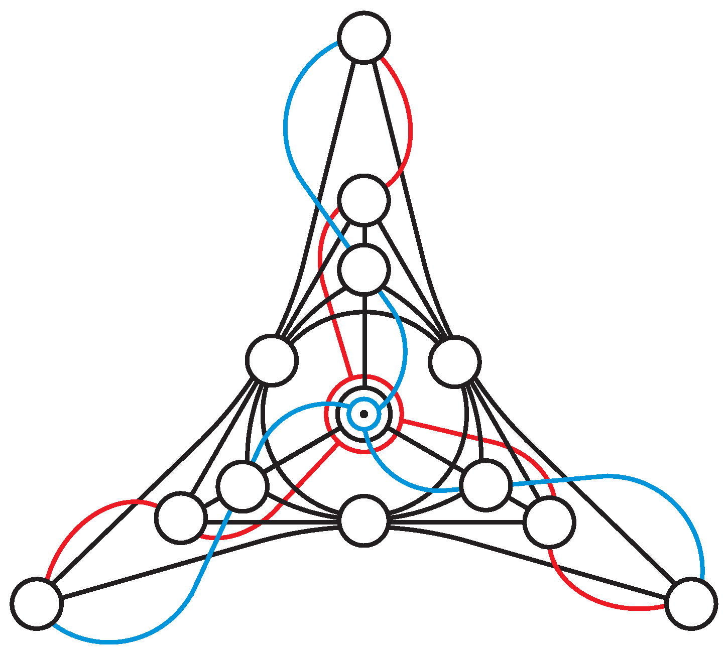
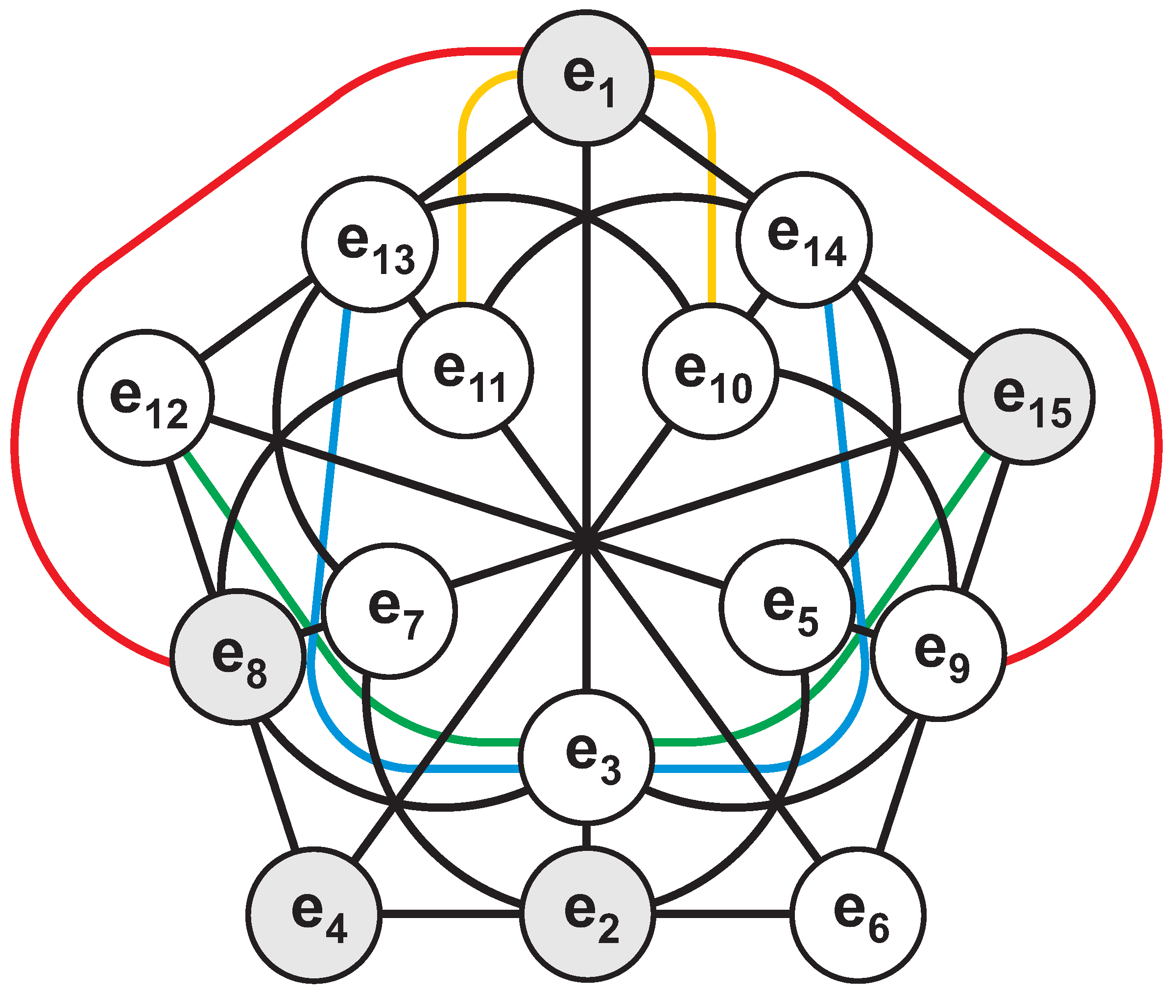
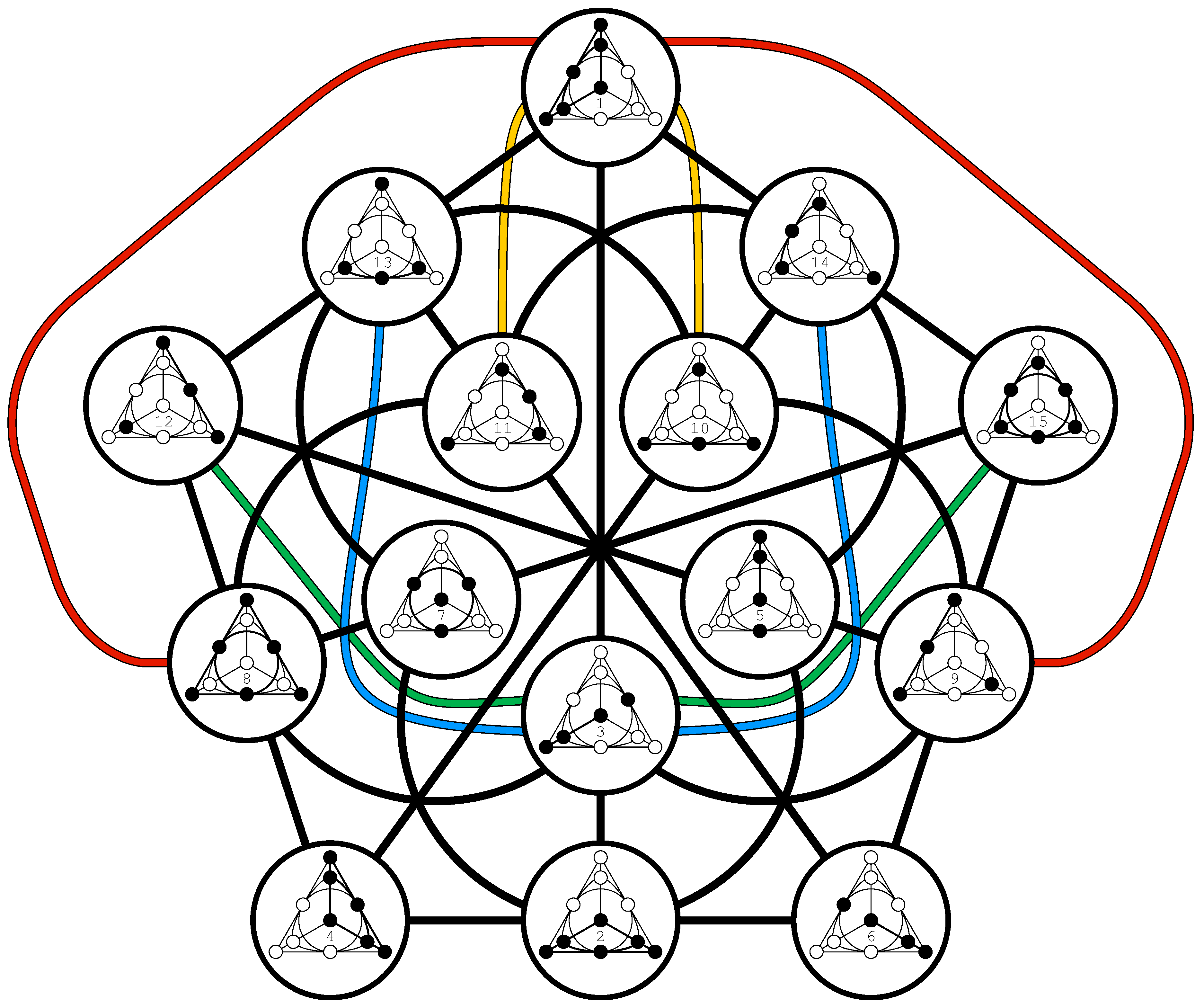
Figure 12.
An illustration of the structure of the -configuration, built around the model of the Desargues configuration shown in Figure 6. The five points added to the Desargues configuration are the three peripheral points and the red and blue point in the center. The 10 lines added are three lines denoted by red color, three blue lines, three lines joining pairwise the three peripheral points and the line that comprises the three points in the center of the figure, that is the ones represented by a bigger red circle, a smaller blue circle and a medium-sized black one.

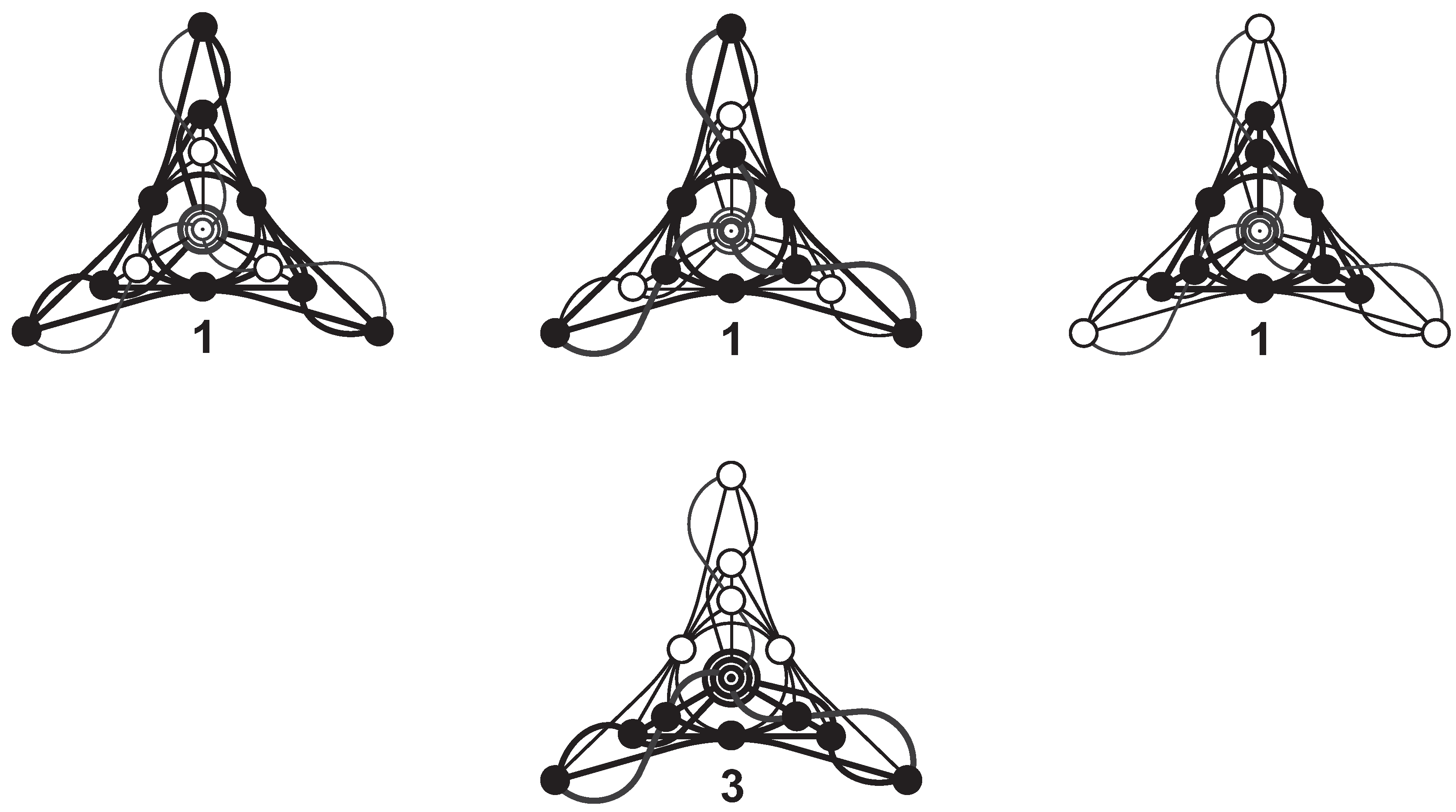
Figure 13.
The 10 geometric hyperplanes of the -configuration of type one; the number below a subfigure indicates how many copies of the particular hyperplane we get by rotating the corresponding subfigure through 120 degrees around its center.
Figure 13.
The 10 geometric hyperplanes of the -configuration of type one; the number below a subfigure indicates how many copies of the particular hyperplane we get by rotating the corresponding subfigure through 120 degrees around its center.
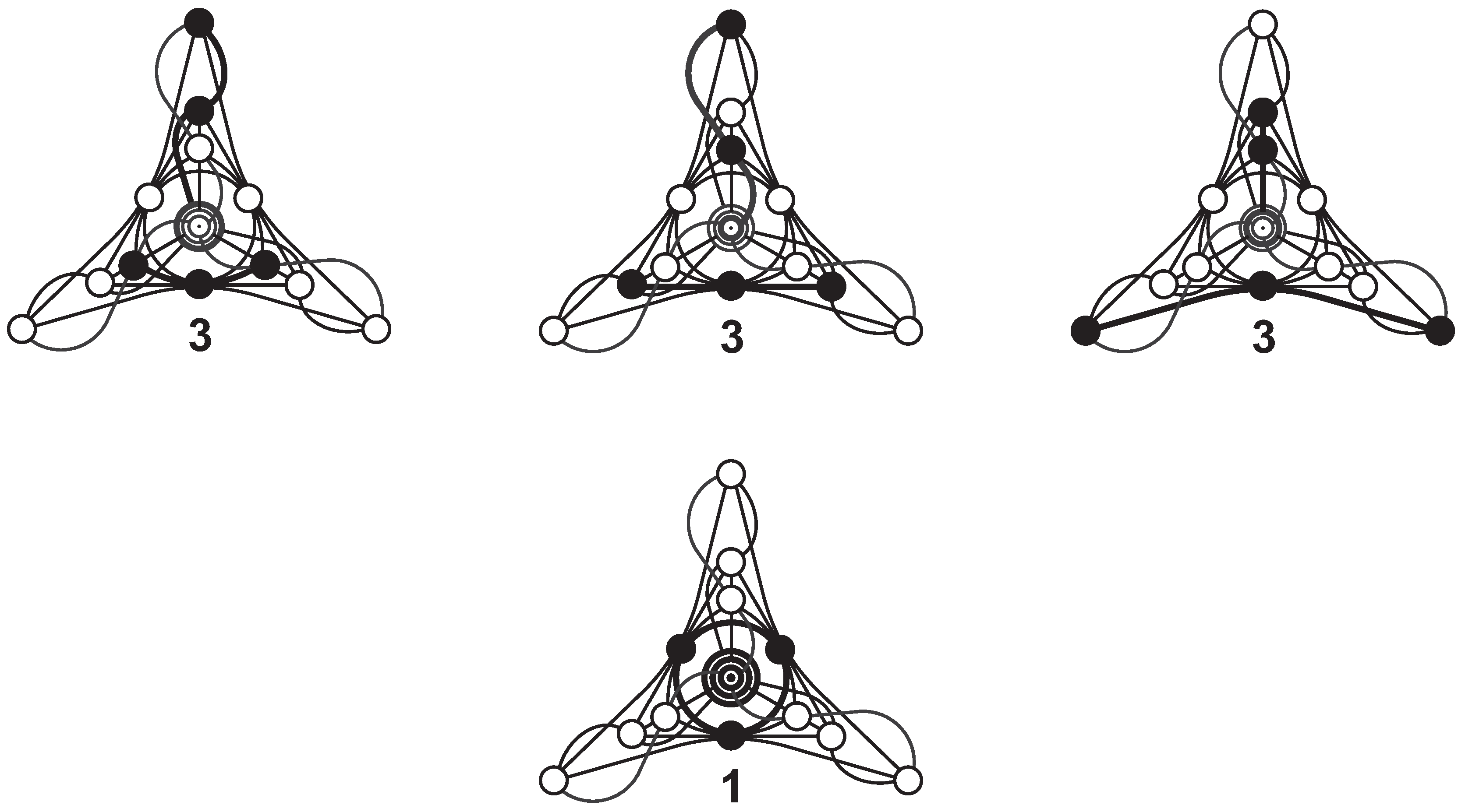
Figure 14.
The 15 geometric hyperplanes of the -configuration of type two.
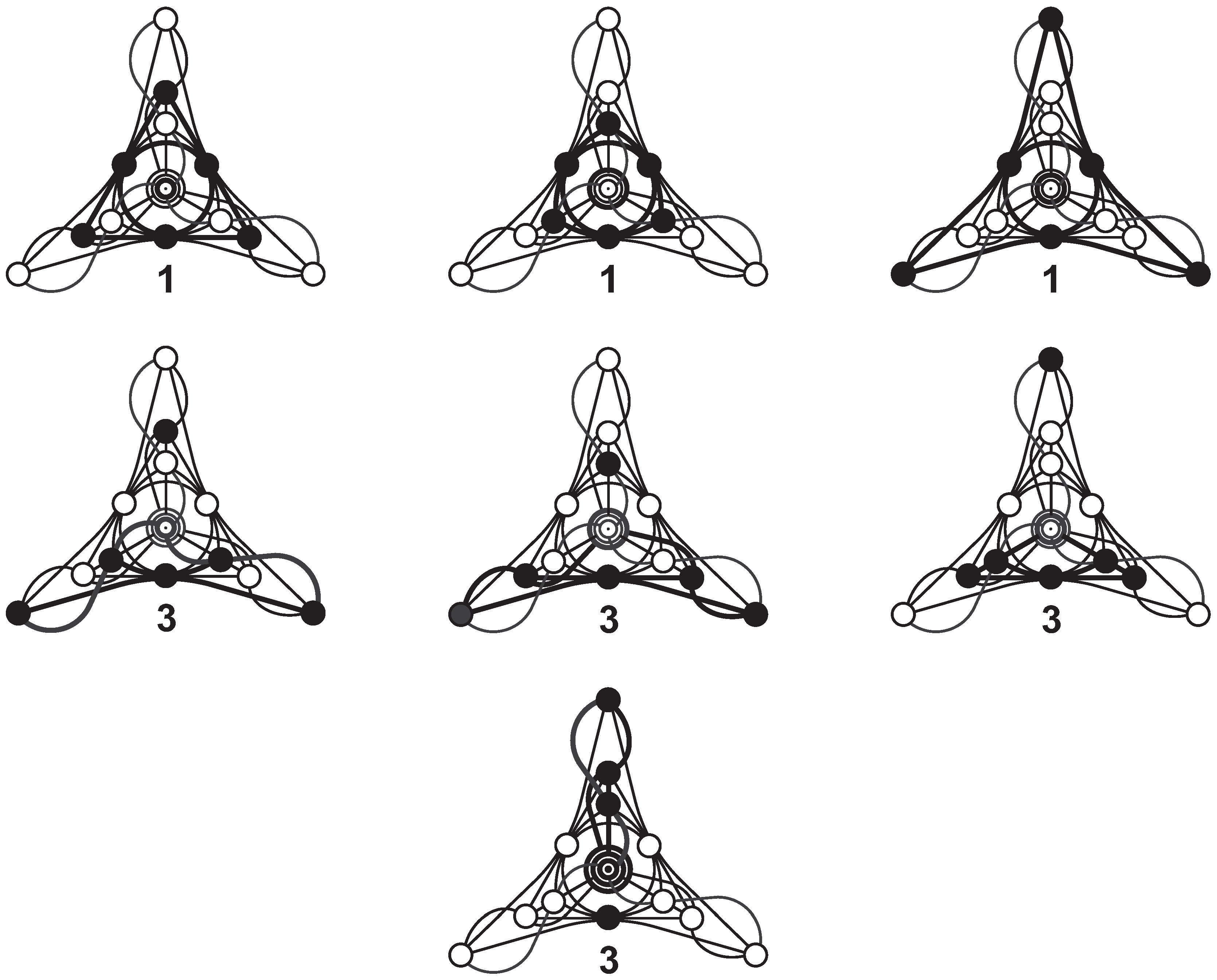
Figure 15.
The six geometric hyperplanes of the -configuration of type three.

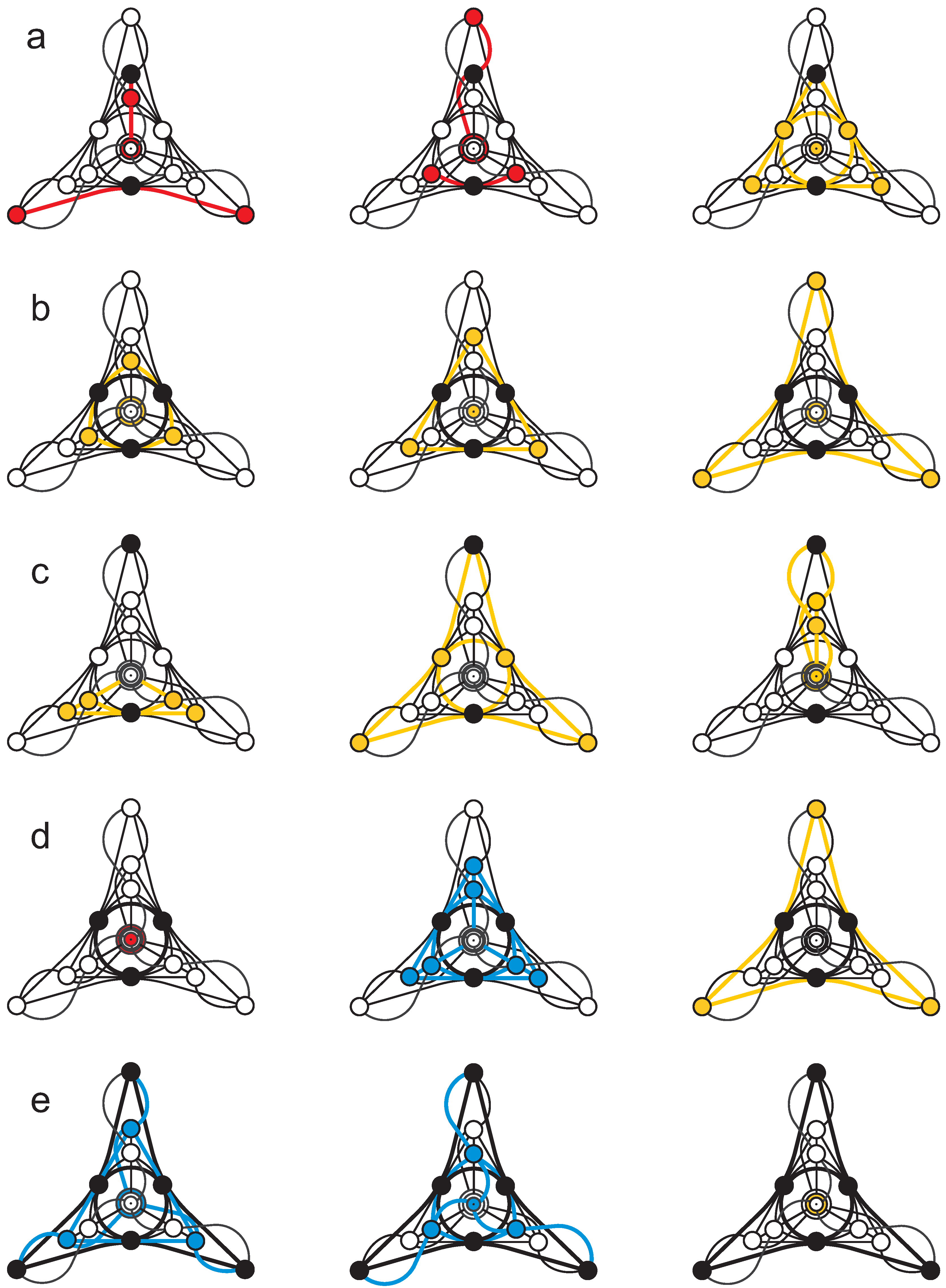
Figure 16.
The five types of Veldkamp lines of the -configuration. Here, unlike Figure 8, Figure 9 and Figure 10, each representative of a geometric hyperplane is drawn separately and different colors are used to distinguish between different hyperplane types: red is reserved for type one, yellow for type two and blue for type three hyperplanes. As before, the black color denotes the core of a Veldkamp line, that is the elements common to all the three hyperplanes comprising it.

We also find that our -configuration yields 155 Veldkamp lines that are, as expected, of five different types. A type-I Veldkamp line, shown in Figure 16a, features two hyperplanes of type one and a type-two hyperplane and its core consists of two points that are at maximum distance from each other; there are Veldkamp lines of this type and they correspond to defective lines of PG of type . A type-II Veldkamp line, featured in Figure 16b, is composed of three hyperplanes of type two that share three points on a common line; there are, obviously, 20 Veldkamp lines of this type, having for their counterparts defective lines of PG of type . A type-III Veldkamp line, portrayed in Figure 16c, also consists of three hyperplanes of type two, but in this case the three common points are pairwise at maximum distance from each other; a quick count leads to 15 Veldkamp lines of this type, these being in a bijection with 15 ordinary lines of PG of type . Next, we have a type-IV Veldkamp line, depicted in Figure 16d, which exhibits a hyperplane of each type and whose core is composed of a line and a point at the maximum distance from it; since for each line of our -configuration there are three points at maximum distance from it, there are Veldkamp lines of this type, having their twins in ordinary lines of PG of type . Finally, we meet a type-V Veldkamp line, sketched in Figure 16e, which is endowed with two hyperplanes of type three and a single one of type two, and whose core is isomorphic to the Pasch configuration; hence, we have Veldkamp lines of this type, being all representatives of ordinary lines of PG of type .
Before embarking on the final case to be dealt with in detail, it is worth having a closer look at our -configuration and pointing out its intimate relation with the famous Pascal’s Mystic Hexagram. If six arbitrary points are chosen on a conic section and joined by line segments in any order to form a hexagon, then the three pairs of opposite sides of the hexagon meet in three points that lie on a straight line, the latter being called the Pascal line. Taking the permutations of the six points, one obtains 60 different hexagons. Thus, the so-called complete Pascal hexagon determines altogether 60 Pascal lines, which generate a remarkable configuration of 146 points and 110 lines called the hexagrammum mysticum, or the complete Pascal figure (for the most comprehensive, applet-based representation of this remarkable geometrical object, see [15]). Both the points and lines of the complete Pascal figure split into several distinct families, usually named after their discoverers in the first half of the 19-th century. We are concerned here with the 15 Salmon points and the 20 Cayley lines (see, for example, [16,17]) which form a -configuration. This configuration is discussed in some detail in [18], where it is also depicted (Figure 6) and called the Cayley-Salmon -configuration. It is precisely this Cayley-Salmon -configuration which our 32-nionic -configuration is isomorphic to. The same configuration is also portrayed in Figure 8 of [15]. In the latter work, two different views/interpretations of the configuration are also mentioned. One is as three pairwise-disjoint triangles that are in perspective from a line, in which case the centers of perspectivity are guaranteed by Desargues’ theorem to also lie on a line; we just stress here that these two lines form a geometric hyperplane (of type one, see Figure 13). The other view of the figure takes any point of the configuration to be the center of perspectivity of two quadrangles whose six pairs of corresponding sides meet necessarily in the points of a Pasch configuration; again, the point and the associated Pasch configuration form a geometric hyperplane (of type two, see Figure 14). We can offer one more view of the configuration, stemming from the existence of type-three hyperplanes, namely as the incidence sum of a Desargues configuration and three triangles on a commmon side (see Figure 15).
5. 64-Nions and a -Configuration
The final algebra we shall treat in sufficient detail is , or the 64-nions. From the corresponding multiplication table, which due to its size we do not show here but which is freely available at [19], we infer the existence of 651 distinguished triples of imaginary units. Regarding the 63 imaginary units of 64-nions as points and the 651 distinguished triples of them as lines, we obtain a point-line incidence structure where each line has three points and each point is on 31 lines, and which is isomorphic to PG. Following the usual procedure, we find that 350 lines of this space are defective and 301 ordinary. Likewise the preceding case, we encounter three different types of points in our 64-nionic PG: 35 α-points, each of which is on 21 defective and 10 ordinary lines; 21 β-points, each of which is on 15 defective and 16 ordinary lines; and seven γ-points, each of them being on 31 ordinary (and, hence, on zero defective) lines. This stratification of the point-set of PG leads, in turn, to three different kinds of defective lines and four distinct kinds of ordinary lines. Out of 350 defective lines, we find 105 of type , 210 of type and 35 of type . On the other hand, 301 ordinary lines are partitioned into 105 lines of type , 70 of type , 105 of type and 21 of type .
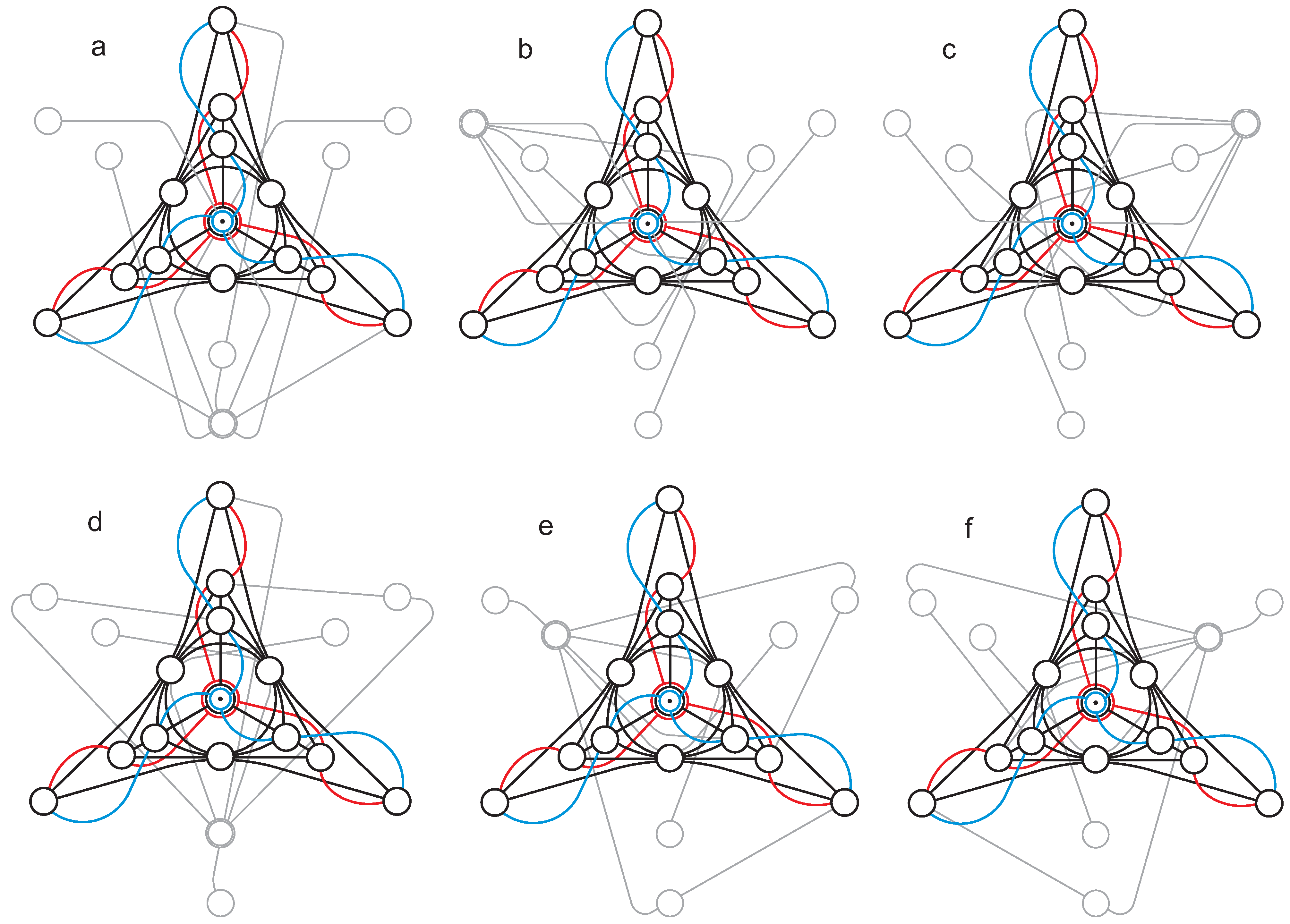
The Veldkamp space mimicking such a fine structure of PG is that of a particular -configuration, , that also lives in our PG and whose points are the 21 β-points and whose lines are the 35 defective lines of type. To visualise this configuration, we build it around the model of the Cayley-Salmon -configuration of 32-nions shown in Figure 12. Given the Cayley-Salmon configuration, there are six points and 15 lines to be added to yield our -configuration, and this is to be done in such a way that the configuration we started with forms a geometric hyperplane in it. As putting all the lines into a single figure would make the latter look rather messy, in Figure 17 we briefly illustrate this construction by drawing six different figures, each featuring all six additional points (gray) but only five out of 15 additional lines (these lines being also drawn in gray color), namely those passing through a selected additional point (represented by a doubled circle). Employing this handy diagrammatical representation, one can verify that our -configuration exhibits 63 geometric hyperplanes that fall into three distinct types. A type-one hyperplane consists of a line and its complement, which is the Pasch configuration; there are 35 distinct hyperplanes of this form, each corresponding to an α-point of our PG. A type-two hyperplane comprises a point and its complement, which is the Desargues configuration; there are 21 hyperplanes of this form, each having a β-point for its PG counterpart. Finally, a type-three hyperplane is isomorphic to the Cayley-Salmon configuration; there are seven distinct hyperplanes of this type, each answering to a γ-point of the PG. We leave it with the interested reader to verify by themselves that the Veldkamp space of our -configuration indeed features 651 lines that do fall into the above-mentioned seven distinct kinds.
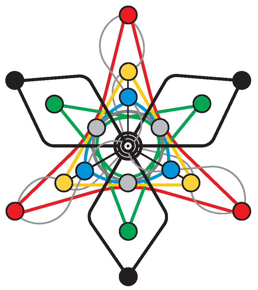
As in the previous two cases, we shall briefly describe a couple of interesting views of our -configuration, both related to type-one hyperplanes. The first one is as four triangles in perspective from a line where the points of perspectivity of six pairs of them form a Pasch configuration, the line and the Pasch configuration comprising a geometric hyperplane (compare with the first view of both the Desargues and the Cayley-Salmon configuration). This is sketched in Figure 18, where the four triangles are denoted, in boldfacing, by green, red, yellow and blue color, the line of perspectivity by boldfaced gray color, and the points of perspectivity of pairs of triangles (together with the corresponding lines they lie on and that are also boldfaced) by black color. The other view is as three complete quadrangles that are pairwise in perspective in such a way that the three points of perspectivity lie on a line and where the six triples of their corresponding sides meet at points located on a Pasch configuration, again the line and the Pasch configuration forming a geometric hyperplane (compare with the second view of both the Desargues and the Cayley-Salmon configuration).
Figure 17.
An illustration of the structure of the -configuration, built around the model of the Cayley-Salmon -configuration shown in Figure 12.
Figure 17.
An illustration of the structure of the -configuration, built around the model of the Cayley-Salmon -configuration shown in Figure 12.

Figure 18.
A “generalized Desargues” view of the -configuration.
6. -Nions and a -Configuration
At this point it is quite easy to spot the general pattern. If one also includes the trivial cases of complex numbers (), where the relevant geometry is just a single point, that is, the -configuration, and quaternions (), whose geometry is a single line, that is, the -configuration, we obtain the following nested sequence of configurations whose Veldkamp spaces capture the stratification/partition of the point- and line-sets of the -nionic PG, N being a positive integer,
It is curious to notice that the first entry represents a triangular number, while the second one is a tetrahedral number, or triangular pyramidal number. In other words, we get a nested sequence of binomial -configurations with and , whose properties have very recently been discussed in a couple of interesting papers [20,21]. The first few configurations are shown, in a form where the configurations are nested inside each other, in Figure 19.
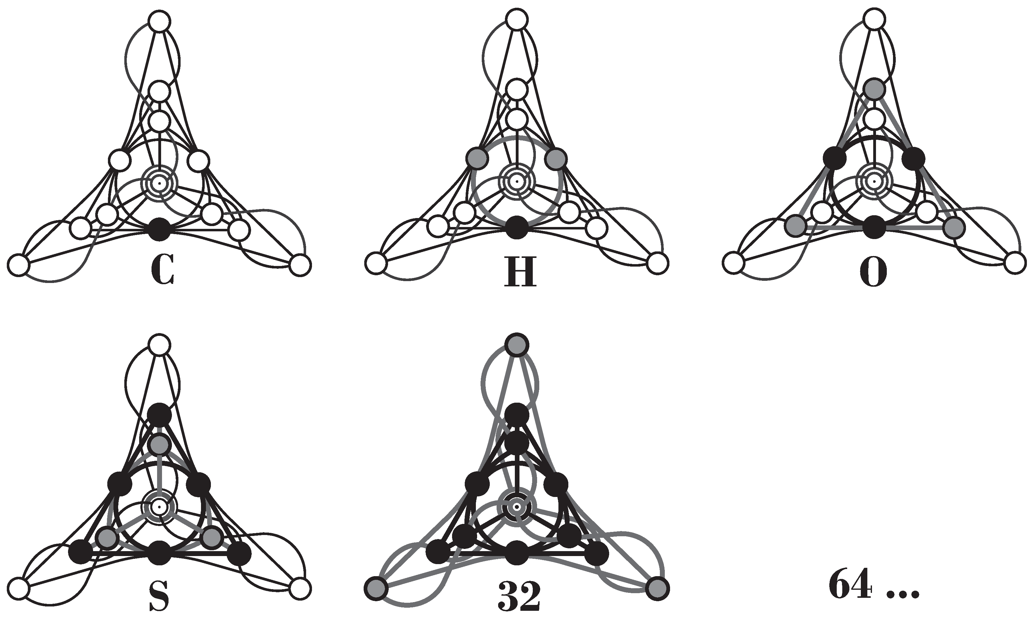
Figure 19.
A nested hierarchy of finite -configurations of -nions for when embedded in the Cayley-Salmon configuration ().
Figure 19.
A nested hierarchy of finite -configurations of -nions for when embedded in the Cayley-Salmon configuration ().

A particular character of this nesting is reflected in the structure of geometric hyperplanes. Denoting our generic -configuration by , we can express the types of geometric hyperplanes of the above-discussed cases in a compact form as follows:
which implies the following generic hyperplane compositions:
or
according as N is even or odd, respectively; here, the symbol “⊔” stands for a disjoint union of two sets.
| : | ⌀, | ||
| : | , | ||
| : | , | , | |
| : | , | , | |
| : | , | , | , |
| : | , | , |
| : | , | , | , | …, |
| : | , | , | , | …, |
In the spirit of previous sections, let us also have a closer look at the nature of our generic . To this end, we first recall the following observations. , the Desargues configuration, can be viewed as () two triangles in perspective from a line which are also perspective from a point, that is ; the line and the point form a geometric hyperplane of . Next, , the Cayley-Salmon configuration, admits a view as () three triangles in perspective from a line where the points of perspectivity of three pairs of them are on a line, aka ; the two lines form a geometric hyperplane of . Finally, , our -configuration, can be treated as () four triangles in perspective from a line where the points of perspectivity of six pairs of them lie on a Pasch configuration, alias ; the line and the Pasch configuration form a geometric hyperplane of . Generalizing these observations, we conjecture that for any , can be regarded as triangles that are in perspective from a line in such a way that the points of perspectivity of pairs of them form the configuration isomorphic to , where the latter and the axis of perspectivity form a geometric hyperplane of .
Next, we invoke the concept of combinatorial Grassmannian (see, for example, [22,23]). Briefly, a combinatorial Grassmannian , where k is a positive integer and X is a finite set, is a point-line incidence structure whose points are k-element subsets of X and whose lines are -element subsets of X, incidence being inclusion. It is known [22] that if and , is a binomial -configuration; in particular, is the Pasch configuration, is the Desargues configuration and ’s with are called generalized Desargues configurations. Now, from our detailed examination of the four cases it follows that , , , , …, are endowed with 1, 5, 15, 35, …, Pasch configurations. And as is also the number of Pasch configurations in , , we are also naturally led to conjecture that . From what we have found in the previous sections it follows that this property indeed holds for , being illustrated for and in Figure 20.
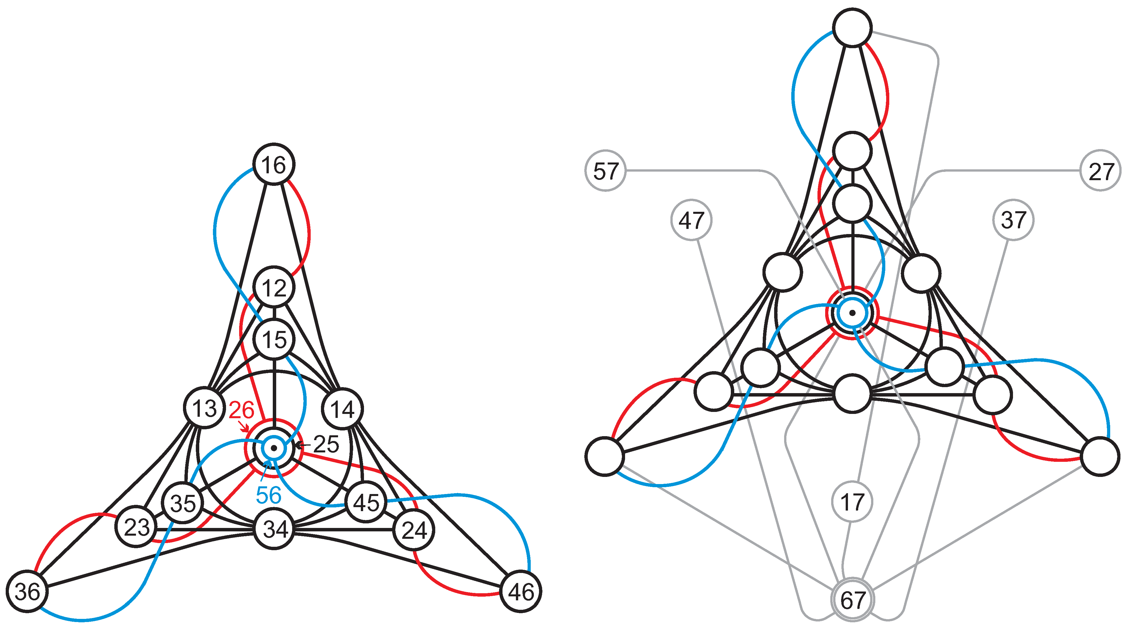
Figure 20.
Left: A diagrammatical proof of the isomorphism between and . The points of are labeled by pairs of elements from the set in such a way that each line of the configuration is indeed of the form , . Right: A pictorial illustration of . Here, the labels of six additional points are only depicted, the rest of the labeling being identical to that shown in the left-hand side figure.

7. Conclusions
An intriguing finite-geometrical underpinning of the multiplication tables of Cayley-Dickson algebras , , has been found that admits generalization to any higher-dimensional . This started with an observation that the multiplication properties of imaginary units of the algebra are encoded in the structure of the projective space PG. Next, this space was shown to possess a refined structure stemming from particular properties of triples of imaginary units forming its lines. To account for this refinement, we employed the concept of Veldkamp space of point-line incidence structure and found out the latter to be a binomial -configuration ; in particular, (octonions) was found to be isomorphic to the Pasch -configuration, (sedenions) to the famous Desargues -configuration, (32-nions) to the Cayley-Salmon -configuration found in the well-known Pascal mystic hexagram and (64-nions) was shown to be identical with a particular -configuration that can be viewed as four triangles in perspective from a line where the points of perspectivity of six pairs of them form a Pasch configuration. These configurations are seen to form a remarkable nested pattern, where is embedded in as its geometric hyperplane, that naturally reflects the spirit of the Cayley-Dickson recursive construction of corresponding algebras.
It is a well-known fact that the only first four algebras , , are “well-behaved” in the sense of being normed, alternative and devoid of zero-divisors—the facts that are frequently offered as an explanation why a relatively little attention has been paid so far to their higher-dimensional cousins, these latter being even regarded by some scholars as “pathological”. It may well be that our finite-geometric, Veldkamp-space-based approach will be able to shed a novel, unexpected light at this issue as it is only starting with when is found to feature a “generalized Desargues property” in the sense that it can be interpreted as triangles that are in perspective from a line in such a way that the points of perspectivity of pairs of them form the configuration isomorphic to . Or, in a slightly different form, it is only for when contains Desargues configurations, these occurring as components of its geometric hyperplanes at that.
Acknowledgments
This work was partially supported by the VEGA Grant Agency, Project 2/0003/13, as well as by the Austrian Science Fund (Fonds zur Förderung der Wissenschaftlichen Forschung (FWF)), Research Project M1564-N27. We would like to express our sincere gratitude to Hans Havlicek (Vienna University of Technology) for a number of critical remarks on the first draft of the paper. Our special thanks go to Jörg Arndt who computed for us multiplication tables of octonions, sedenions, 32-nions and 64-nions. We are also very grateful to Boris Odehnal (University of Applied Arts, Vienna) for creating nice computer versions of several figures.
Author Contributions
Metod Saniga and Frédéric Holweck conducted research, Metod Saniga wrote the paper and Petr Pracna computerized a diagrammatical presentation of the main results.
Conflicts of Interest
The authors declare no conflict of interest.
References
- Jacobson, N. Basic Algebra I; W. H. Freeman: San Francisco, CA, USA, 1974. [Google Scholar]
- Schafer, R.D. Introduction to Non-Associative Algebras; Dover: New York, NY, USA, 1995. [Google Scholar]
- Moreno, G. Hopf construction map in higher dimensions. Bol. Soc. Mat. Mex. 2004, 10, 383–397. [Google Scholar]
- Arndt, J. Matters Computational: Ideas, Algorithms, Source Code; Springer: Heidelberg, Germany, 2011. [Google Scholar]
- Arndt, J. The FXT Demos: Arithmetical Algorithms. Available online: http://jjj.de/fxt/demo/arith/index.html (accessed on 30 January 2014).
- Baez, J.C. The octonions. Bull. Am. Math. Soc. 2002, 39, 145–205. [Google Scholar] [CrossRef]
- Culbert, C. Cayley-Dickson algebras and loops. J. Gen. Lie Theory Appl. 2007, 1, 1–17. [Google Scholar] [CrossRef]
- Shult, E.E. Points and Lines: Characterizing the Classical Geometries; Springer: Berlin, Germany, 2011. [Google Scholar]
- Grünbaum, B. Configurations of Points and Lines; Graduate Studies in Mathematics 103; American Mathematical Society: Providence, RI, USA, 2009. [Google Scholar]
- Buekenhout, F.; Cohen, A.M. Diagram Geometry: Related to Classical Groups and Buildings; Springer: Berlin, Germany, 2013. [Google Scholar]
- Grannell, M.J.; Griggs, T.S. The Pasch Configuration. Encyclopaedia of Mathematics. Available online: http://www.encyclopediaofmath.org/index.php/Pasch_configuration (accessed on 14 May 2014).
- Polster, B. A Geometrical Picture Book; Springer Verlag: New York, NY, USA, 1998. [Google Scholar]
- Pisanski, T.; Servatius, B. Configurations from a Graphical Viewpoint; Birkhäuser: Basel, Switzerland, 2013. [Google Scholar]
- Saniga, M.; Planat, M.; Pracna, P.; Havlicek, H. The Veldkamp space of two-qubits. SIGMA 2007, 3. [Google Scholar] [CrossRef]
- Fisher, J.C.; Fuller, N. The Complete Pascal Figure Graphically Presented. Available online: http://www.math.uregina.ca/˜fisher/Norma/paper.html (accessed on 14 May 2014).
- Lord, E. Symmetry and Pattern in Projective Geometry; Springer: Heidelberg, Germany, 2013. [Google Scholar]
- Conway, J.; Ryba, A. The Pascal mysticum demystified. Math. Intell. 2012, 34, 4–8. [Google Scholar] [CrossRef]
- Boben, M.; Gévay, G.; Pisanski, T. Danzer’s configuration revisited. Adv. Geom. 2015, 15, 393–408. [Google Scholar] [CrossRef]
- Arndt, J. TMP-Zero-Divisors. Available online: http://jjj.de/tmp-zero-divisors/mult-table-64-ions.txt (accessed on 30 January 2014).
- Prażmowska, M.; Prażmowski, K. Binomial Configurations Which Contain Complete Graphs: Kn-Subgraphs of a -Configuration. 2014. arXiv:1404.4064. Available online: http://arxiv.org/abs/1404.4064 (accessed on 17 May 2014).
- Petelczyc, K.; Prażmowska, M.; Prażmowski, K. A complete classification of the ()-configurations with at least three K5-graphs. Discret. Math. 2015, 338, 1243–1251. [Google Scholar] [CrossRef]
- Prażmowska, M. Multiple perspectives and generalizations of the Desargues configuration. Demonstr. Math. 2006, 39, 887–906. [Google Scholar]
- Prażmowska, M.; Prażmowski, K. A generalization of Desargues and Veronese configurations. Serdica Math. J. 2006, 32, 185–208. [Google Scholar]
© 2015 by the authors; licensee MDPI, Basel, Switzerland. This article is an open access article distributed under the terms and conditions of the Creative Commons Attribution license (http://creativecommons.org/licenses/by/4.0/).
Share and Cite
MDPI and ACS Style
Saniga, M.; Holweck, F.; Pracna, P. From Cayley-Dickson Algebras to Combinatorial Grassmannians. Mathematics 2015, 3, 1192-1221. https://doi.org/10.3390/math3041192
AMA Style
Saniga M, Holweck F, Pracna P. From Cayley-Dickson Algebras to Combinatorial Grassmannians. Mathematics. 2015; 3(4):1192-1221. https://doi.org/10.3390/math3041192
Chicago/Turabian StyleSaniga, Metod, Frédéric Holweck, and Petr Pracna. 2015. "From Cayley-Dickson Algebras to Combinatorial Grassmannians" Mathematics 3, no. 4: 1192-1221. https://doi.org/10.3390/math3041192