Article

Optimization of Truck–Cargo Online Matching for the Less-Than-Truck-Load Logistics Hub under Real-Time Demand

1
Key Laboratory of Transport Industry of Big Data Application Technologies for Comprehensive Transport, School of Traffic and Transportation, Beijing Jiaotong University, Beijing 100044, China
2
China North Artificial Intelligence & Innovation Research Institute, Beijing 100072, China
*
Author to whom correspondence should be addressed.
Mathematics 2024, 12(5), 755; https://doi.org/10.3390/math12050755
Submission received: 8 February 2024 / Revised: 28 February 2024 / Accepted: 29 February 2024 / Published: 2 March 2024

Abstract

:
Reasonable matching of capacity resources and transported cargoes is the key to realizing intelligent scheduling of less-than-truck-load (LTL) logistics. In practice, there are many types and numbers of participating objects involved in LTL logistics, such as customers, orders, trucks, unitized implements, etc. This results in a complex and large number of matching schemes where truck assignments interact with customer order service sequencing. For the truck–cargo online matching problem under real-time demand, it is necessary to comprehensively consider the online matching process of multi-node orders and the scheduling of multi-types of trucks. Combined with the actual operation scenario, a mixed-integer nonlinear programming model is introduced, and an online matching algorithm with a double-layer nested time window is designed to solve it. By solving the model in a small numerical case using Gurobi and the online matching algorithm, the validity of the model and the effectiveness of the algorithm are verified. The results indicate that the online matching algorithm can obtain optimization results with a lower gap while outperforming in terms of computation time. Relying on the realistic large-scale case for empirical analysis, the optimization results in a significant reduction in the number of trips for smaller types of trucks, and the average truck loading efficiency has reached close to 95%. The experimental results demonstrate the general applicability and effectiveness of the algorithm. Thus, it helps to realize the on-demand allocation of capacity resources and the timely response of transportation scheduling of LTL logistics hubs.

1. Introduction

Freight transportation is a vital element in national, regional, and municipal economies [1]. Road freight has become the dominant mode of transportation, supporting regional economic growth, providing door-to-door transportation, and having the advantages of being extremely convenient, flexible, and fast. From the regional distribution of global road freight market share, according to statistics, China ranked first with a 31.81% share in 2022. In terms of China’s market scale, the proportion of the four modes of freight transportation in recent years is shown in Figure 1. The share of road freight transport has declined slightly, but it still occupies a dominant position in China’s transportation system.
The three main modes of the road freight logistics industry are Express, LTL logistics, and full-truck-load (FTL) logistics. A comparison of the characteristics of the three modes is shown in Table 1. Generally, LTL logistics handles shipments larger than express but less than FTL logistics [2]. LTL logistics is for shipments that weigh or have a volume less than one truckload resulting from trucks that run partially filled and need to be assembled and transported with other shipments. In 2023, the road freight market of China will reach RMB 6 trillion. Of this, the market size of express, LTL logistics, and FTL logistics is about RMB 0.9 trillion, RMB 1.5 trillion, and RMB 3.2 trillion, respectively [3]. In the last decade, the share of LTL logistics within the road freight industry has grown due to economic trends [4]. However, LTL logistics has been facing a developing bottleneck, in particular the imbalance between supply and demand as well as the blockage of information flow, owing to unreasonable and insufficient allocation of logistics resources. The competitive environment forcing logistics service providers to offer services at lower prices and tactical planning of operations is becoming increasingly important for the company to achieve its economic goals. Tactical planning consists of a series of interrelated decisions and is aimed to achieve the optimal utilization of resources. In the operation of an LTL logistics hub, truck–cargo matching and truck scheduling decisions are a series of interrelated tactical decisions.
The in-city pickup business operation of an LTL logistics hub is mainly oriented to the freight demand within the city. Trucks are generally used for transporting goods, while unitized implements are used for loading goods. It facilitates mechanized loading and unloading operations and improves operational efficiency. Smaller shipments of LTL logistics are consolidated to obtain a full truckload, and the sharing of trucks can reduce the number of trucks used. The traditional scheduling process is usually accomplished manually and relies on the subjective experience and skills of the dispatchers. As freight quantities are uncertain, the dispatchers dynamically decide order–truck matching and truck scheduling on real-time operations [5], which makes scheduling optimization difficult. Meanwhile, due to the operational characteristics of LTL logistics, numerous orders are generated in real time, and a large number of small shipments require sharing trucks. Conducting efficient online truck–cargo matching increases truck utilization efficiency and reduces the number of trucks used, which, in return, improves the operational efficiency of LTL logistics hubs. This study investigates the problem of the LTL truck–cargo matching and truck scheduling problem based on the real uncertain LTL logistics order demand, which has certain theoretical and practical significance.
This paper studied the LTL online truck–cargo matching and truck scheduling problem with scattered logistics nodes, numerous real-time order demands, standardized unitized implements, multiple types of trucks, and time window constraints. Compared with past work, this paper considers the characteristics of LTL logistics where numerous shipment orders are generated in real time and need to consolidate several orders to fill a truck. So, we designed an online matching algorithm and compared its performance with the Gurobi solver in the small numerical case. Using empirical cases, we explored the influence of various factors on the matching results. Our contributions are:
  • In order to respond to the real-time LTL logistics demand, we designed an online matching algorithm. Since information is input and output in real time, and decisions are made based on partial information, theoretically there is no optimal online algorithm. However, small numerical case study demonstrates that the optimization of our algorithm results in a small gap compared to the Gurobi solver but significantly reduces the computing time.
  • The online matching algorithm studied in this paper creatively introduces the double-layer nested time window mechanism. In the empirical case, we verified the effectiveness of the double-layer nested time window and conducted sensitivity analysis of other algorithm parameters. In addition, the scenario of zone partitioning is considered, which shows that for this problem, the judgment of the algorithm performs better without zone partitioning.
The remainder of this study is as follows: Section 2 presents an overview of the relevant literature. Section 3 defines the problem, and a mixed-integer nonlinear programming formulation is constructed. Section 4 introduces an online matching algorithm to solve the problem under the condition of real-time orders and multiple types of trucks. In Section 5, we conduct numerical experimental studies on two cases. Gurobi is used to solve a small numerical case to validate the validity of the model and the algorithm. The effectiveness of the algorithm is demonstrated by empirical case studies. Section 6 summarizes the findings and outlines potential future research extensions.

2. Literature Review

The optimization of truck–cargo online matching for the LTL logistics hub under real-time demand studied in this paper mainly involves two aspects of scientific problems: the truck–order–cargo matching schemes and the truck scheduling problem, that is, the simultaneous consideration of the dispatch time and the specific visit routes of trucks in the matching process to achieve a better optimization goal. Therefore, this section reviews the relevant research on logistics vehicle scheduling problems and vehicle–cargo matching problems in recent years and summarizes the research features and future research directions.

2.1. Research on Logistics Vehicle Scheduling Problem

Some recent studies on vehicle scheduling problems for logistics companies are summarized as follows: Giovanni et al. [6] proposed a tool that integrates several modules for small trucking companies. It allows the initial assignment of trucks and service routes, while responding to dynamic events in a timely manner. Shi et al. [7] proposed a combined qualitative and quantitative online intelligent scheduling method to solve the large-scale vehicle routing and scheduling problem in B2C e-commerce urban logistics distribution. Cantarella et al. [8] proposed a modeling approach to multi-vehicle type assignment with resilient vehicle selection behavior, which is applied to analyze the assignment of congested and non-congested networks. Wang et al. [9] considered the multi-warehouse vehicle routing problem and proposed a resource-sharing scheme based on customer clustering to achieve a balanced distribution of spatial resources. Furthermore, Pasha et al. [10] conducted a structured survey of the studies on electric vehicle scheduling, described the operations research aspects and problem-specific attributes, and formulated some representative mathematical models to guide future research. There are also several relevant studies considering the scheduling of logistics vehicles within a restricted area, such as community logistics and in-plant logistics. Ouyang et al. [11] proposed a novel postponement prioritized route optional approach, formulated two dynamic policies to manage temporal and spatial uncertainties, and evaluated the policies through simulation experiments on large-scale instances. Diefenbach et al. [12] proposed a scheduling problem of electric vehicles in an in-plant logistics setting in which the actual battery charging function is considered and proposed an exact approach based on branch-and-check for minimizing the fleet size.
In production scheduling with a delivery problem, researchers have carried out much research on integrated production and distribution scheduling. Low et al. [13] discussed the production scheduling with delivery problems. The retailers need to determine the sequence in which each vehicle is visited to ensure that the goods can be delivered within a certain time window, and a heterogeneous fleet of vehicles is considered. Additionally, Wang et al. [14] considered an integrated single-machine scheduling and multi-vehicle routing problem, and the target is to minimize total carbon emissions. Fathollahi-Fard et al. [15] developed a sustainable distributed permutation flow-shop scheduling model and introduced a novel heuristic based on the social engineering optimizer. The GSC multi-objective integrated scheduling problem for production and distribution is modeled as a mixed-integer non-learning programming formula, considering heterogeneous fleet and batch delivery (Ganji et al. [16]). Yagmur et al. [17] studied a new variant of the integrated production and distribution scheduling problem and emphasized that combining orders in a trip is necessary to reduce the total travel time required by the vehicle.
Furthermore, crowdsourcing and alternative delivery modes, as emerging forms of urban last-mile delivery, help reduce the externalities of urban freight logistics. Kang et al. [18] proposed a method to control orders and schedule the routes of parcel pickup and delivery and used reinforcement learning with artificial neural networks to solve it. Wehbi et al. [19] described an urban delivery system that integrates the routing of vans and porters and proposed an efficient heuristic that produces results in a short computational time. The truck–drone hybrid transportation systems have become a promising solution. Gu et al. [20] investigated the dynamic truck–drone routing problem, and the scheduled deliveries and on-demand pickups were considered. Then the problem is formulated as a Markov decision process.
The literature related to the vehicle scheduling problem is summarized in Table 2.

2.2. Research on Vehicle–Cargo Matching Problem

In the logistics field, vehicle–cargo matching is a key issue in road freight transportation, and scholars have conducted considerable research focused on the problem. Tian et al. [21] proposed a vehicle–cargo matching algorithm based on an improved dynamic Bayesian network. Yu et al. [22] proposed a vehicle–cargo matching model based on the weed optimization algorithm and integrated various factors to establish an objective function for calculation. Wang et al. [23] established a vehicle routing optimization model considering goods–vehicle matching and three-dimensional loading constraints. Yücel et al. [24] introduced a multi-period, two-dimensional vehicle loading and dispatching problem. Order due dates, incompatibility of orders, vehicle capacities, and other constraints are considered. In recent years, many studies have focused on road freight platforms. Li et al. [25] proposed an optimal assignment-matching strategy for a freight O2O platform. In order to study the vehicle–cargo matching problem with heterogeneous demands from vehicle owners, shippers, and platforms in the platform model, Ni et al. [26] introduced the platform demand and proposed a resource-coordinated scheduling optimization method that includes a two-stage model. Deng et al. [27] proposed a resource-coordinated scheduling optimization method that includes a two-stage model, and it is proved that the dynamic nature of sharing resources can effectively solve unbalanced resource competition. Iris et al. [28] addressed the integrated management of ship-loading operations. Stowage planning, load sequencing, planning, and scheduling of the equipment to use are considered.
Matching methods have also been studied in the field of passenger transportation, with the most widely studied being vehicle–passenger matching for online taxis. Agatz et al. [29] focused on dynamic ride-sharing systems and believed that the optimization algorithm was the key technology to achieve real-time matching between drivers and passengers on the ride-hailing platform. Guo et al. [30] presented a matching algorithm that matches drivers and customers based on specific objectives and feasibility constraints given a list of available vehicles and customer-requested trips. Based on that, Zhan et al. [31] proposed a lexicographic multi-objective dynamic ride-hailing sharing program, and multiple vehicle types and user classes are considered. In the context of on-demand ride-hailing, Meshkani et al. [32] proposed a dynamic two-to-one ride-matching algorithm, and a passenger can share their ride with others. Meanwhile, to assign the ride-sharing vehicles while considering network traffic dynamics, Zhou et al. [33] proposed a scalable dynamic ride-sharing method that can solve the endogenous congestion effect. While optimizing vehicle assignment and routing simultaneously, Qin et al. [34] investigated the ride-sharing matching problem in conjunction with predicted near-term pooled information for matching vehicles and passengers in various scenarios over multiple matching iterations.
The literature related to the vehicle–cargo matching problem is summarized in Table 3.

2.3. Contribution Statements

To sum up, scholars have performed extensive detailed research on the analysis of logistics vehicle scheduling problems and vehicle–passenger/cargo matching methods in the field of passenger and freight transportation.
(1) The vehicle–cargo matching method and vehicle scheduling optimization method are always integrated for research.
(2) The current research concentrated on vehicle–cargo matching is mostly based on freight platforms to study the supply–demand matching problem and the vehicle loading problem in FTL logistics. Many studies are limited to static matching and often use heuristic algorithms to solve it, such as the particle swarm algorithm, the weed algorithm, and NSGA II. Some scholars have focused on the dynamic vehicle–cargo matching problem, however, based on complete information input.
(3) The related research on on-demand rides of online taxis highlights the importance of demand. Algorithms are designed to optimize real-time matching of drivers and passengers, and ride-hailing sharing problems are considered by some of the studies.
The LTL logistics involves a large number and real-time, high-frequency generation of small-volume shipment orders that require sharing trucks. It is an extension of the traditional vehicle–cargo matching problem, and the traditional heuristic algorithms cannot be well applied. In this paper, an online matching algorithm is designed to solve the LTL logistics truck–cargo matching and truck scheduling problem, which dynamically responds to the current real-time partial order demand. It is conducive to better matching demand while fully utilizing logistics resources and ensuring a certain level of response efficiency to improve service quality.

3. Problem Definition and Model Formulation

This section describes in detail the LTL truck–cargo matching and truck scheduling problem and summarizes notations at first. Then, a mixed-integer nonlinear programming formulation is developed to solve the problem.

3.1. Problem Description and Assumptions

The LTL truck–cargo matching and truck scheduling problem based on real-time demand data determines the matching relationship between each order and truck, the truck dispatch time, the visit routes of the trucks, and the order service sequence at each pickup node. It is an integration of the vehicle–cargo matching problem and the vehicle scheduling problem.
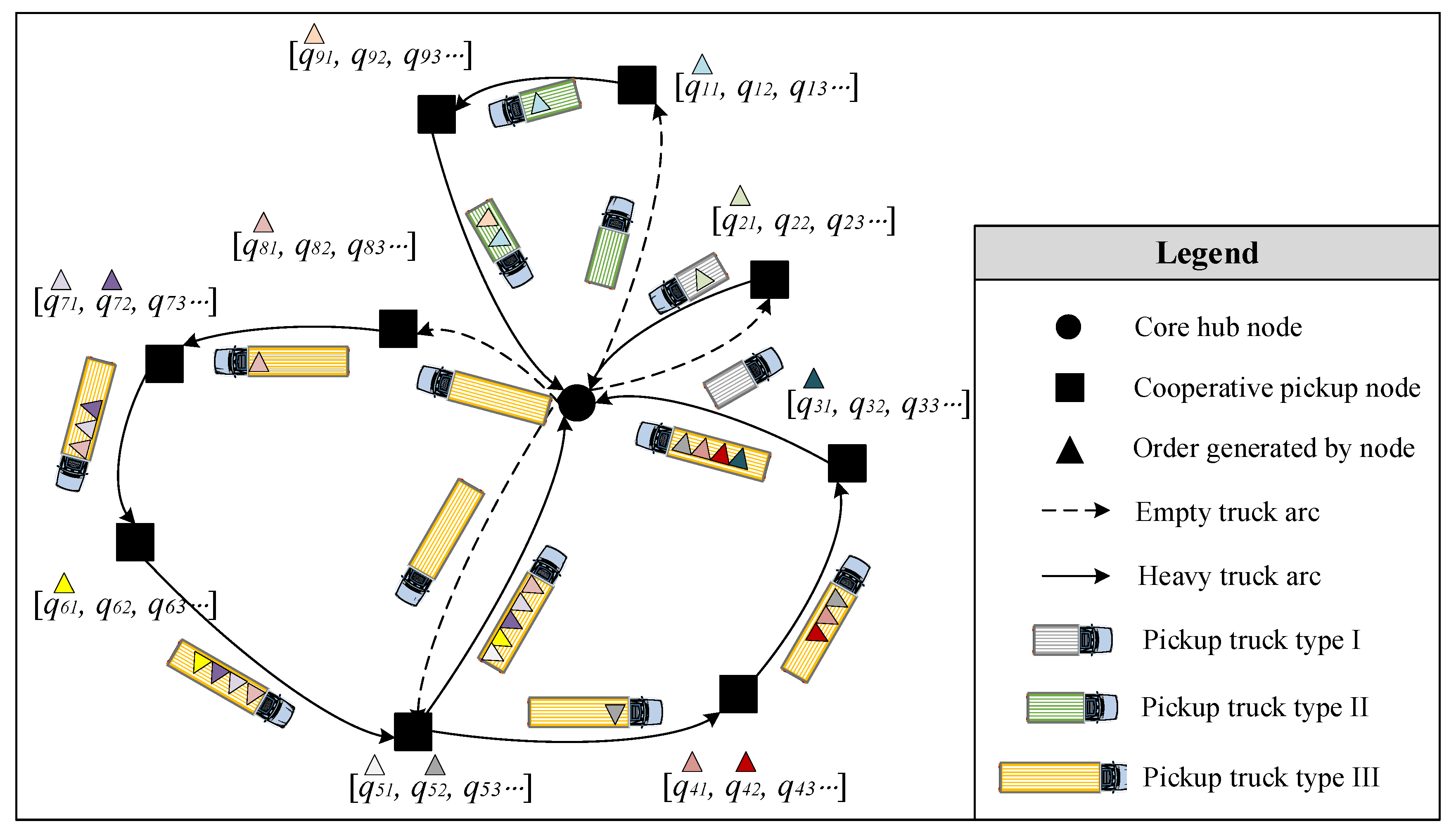
The problem is defined as a directed graph, G ( N , E ) , as shown in Figure 2. N is the set of all logistics nodes, including two types of nodes: core hub node { 0 , n + 1 } , where n + 1 represents the virtual core hub node, and the set of cooperative pickup nodes N . Each cooperative pickup node generates orders in chronological sequence, with independent demand for each order. Cargoes are loaded with uniform specifications of unitized implements and assembled into a unitized unit. The truck fleet has m types of trucks with different capacities. The core hub dispatches the appropriate trucks to visit the corresponding cooperative pickup nodes for unitized unit loading.
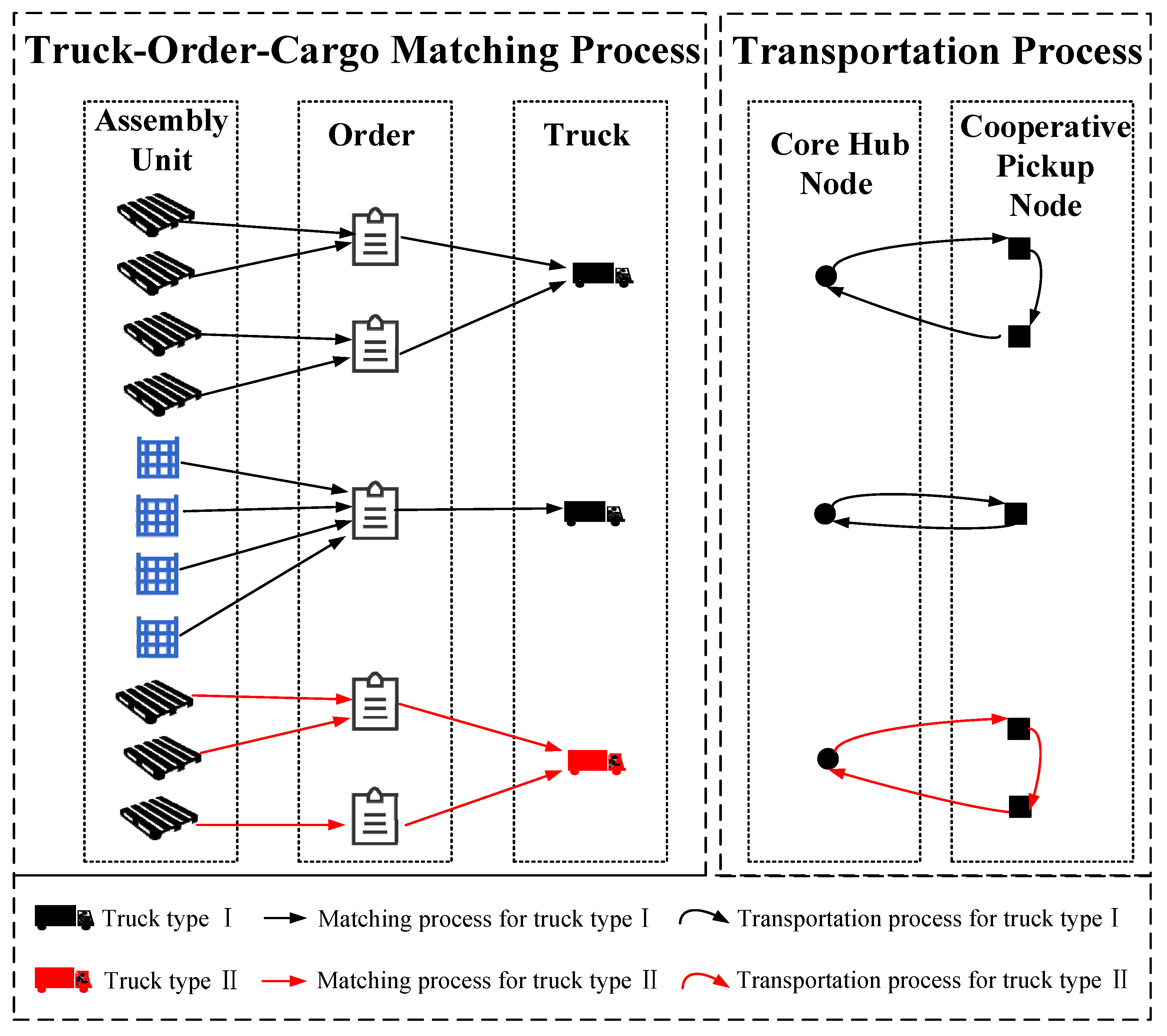
The schematic of the truck–cargo matching process consists of two sub-processes, as shown in Figure 3. The truck–order–cargo matching process indicates that each order demand includes a certain number of unitized units. Multiple orders are consolidated into a waybill for transportation by a specific type of truck. Since a waybill may contain orders generated by multiple cooperative pickup nodes, the transportation process indicates that the truck needs to visit in a certain optimized sequence to service all the assigned orders.
The assumptions of this study are the following:
(1) Each truck can be assigned only one pickup waybill, and the assignment is independent.
(2) All corresponding orders generated by the cooperative pickup nodes must be serviced.
(3) Each type of truck is available in sufficient quantity.
(4) Transportation costs are only related to the distance traveled and the type of truck. Trucks have the same unit transportation cost for heavy and empty loads.
(5) Orders are not allowed to be split for transportation.

3.2. Model Notations

The model notations are listed in Table 4.

3.3. Model Formulation

The objective function:
min f = j N b J j l L k K l c l d i s p a t c h x j b l y 0 j b l k + l L k K l c l t r a n s ( i N a J i j N b J j , b a d i j q i a x i a l x j b l y i a j b l k )
The constraints are divided into five groups, each representing one type of system constraint.
Truck–cargo matching constraints:
l L x i a l = 1 , i N , a J i
l L k K l w i a l k = 1 , i N , a J i
a J i x i a l z i l k q i , i N , l L , k K l
w i a l k z i l k , i N , a J i , l L , k K l
z i l k x i a l , i N , a J i , l L , k K l
Truck scheduling sequence constraints:
s N c J s , c b x j b l x s c l y j b s c l k i N a J i , a b x i a l x j b l y i a j b l k = { 1 l L , k K l , j { 0 } 0 j N , b J j , l L , k K l 1 l L , k K l , j { n + 1 }
l L k K l s N c J s , c b y j b s c l k = 1 , j N , b J j
l L k K l i N c J i , a b y i a j b l k = 1 , j N , b J j
j N b J j y 0 j b l k = j N b J j y j b n + 1 l k , l L , k K j
j N b J j y i a j b l k z i l k , i N , a J i , l L , k K l
j N b J j y j b i a l k z i l k , i N , a J i , l L , k K l
y i a j b l k w i a l k + w j b l k 2 , i , j N , a J i , b J j , a b , l L , k K l
y 0 , n + 1 l k = 0 , l L , k K l
Truck load constraints:
i N a J i q i a w i a l k Q l , l L , k K l
Q i a l k + q i a + Q l ( y i a j b l k 1 ) Q j b l k , i , j N , a J i , b J j , l L , k K l
Q i a l k min { Q l , Q l + q i a } , i N , a J i , l L , k K l
Time window constraints:
T 0 l k = max i N , a J l k ( T i a w i a l k ) , l L , k K l
T 0 l k T i a + T 1 M ( 2 x i a l w i a l k ) , l L , k K l , i N , a J i
0–1 decision variable constraints:
w i a l k { 0 , 1 } , i N , j J i , l L , k K l
z i l k { 0 , 1 } , i N , l L , k K l
x i a l { 0 , 1 } , i N , j J i , l L
y i a j b l k { 0 , 1 } , i , j N , a J i , b J j , b a , l L , k K l
The objective is to minimize operating economic costs, including transportation costs and fixed dispatch costs, as expressed by Equation (1). Fixed dispatch costs are the one-time fixed costs incurred when a truck is put to work on a transportation assignment, which primarily include the access costs, maintenance costs, insurance costs, and the truck driver’s salary. Transportation costs are the costs of fuel consumed by the truck throughout the transportation assignment, which increase as the distance traveled by the truck increases.
The constraints of the model are expressed as follows:
Equations (2)–(6) are truck–cargo matching constraints. Equations (2) and (3) ensure that each order must be serviced once. Equation (4) ensures that for each truck, the number of services at each pickup node is less than or equal to the number of orders generated. Equations (5) and (6) are relationship constraints between decision variables. If z i l k = 1 , then w i a l k = 0 / 1 , otherwise w i a l k = 0 . That is, it is only possible to service the order a at node i if truck k of type l serves node i . As well, if x i a l = 1 , then z i l k = 0 / 1 , otherwise z i l k = 0 .
Equations (7)–(14) are truck scheduling sequence constraints. Equation (7) represents the transportation balance constraints for trucks to ensure the continuity of the front and rear sequential service arcs. All pickup nodes and core hub nodes are considered. Equations (8) and (9) restrict that each order must be serviced by one trip. Equation (10) ensures that the number of trucks departing from the core hub is equal to the number of trucks returned. Equations (11) and (12) ensure that if truck k does not serve pickup node i , it will not depart from or arrive at node i . Equation (13) restricts that node i and node j can be served sequentially only if truck k serves both node i and node j . Equation (14) is the infeasibility constraints for service sequence.
Equations (15)–(17) are truck load constraints. Equation (15) represents the loading capacity limit of the trucks, that is, the total number of unitized units loaded on the truck must be less than or equal to the truck capacity. Equation (16) represents the constraints used to eliminate subloops. Equation (17) restricts the load of truck k after serving each order.
Equations (18) and (19) are time window constraints. Equation (18) represents the departure time of truck k from the core hub (i.e., the order processing time of the order served by truck k ), which is the latest generation time among the orders it serves. Equation (19) is a hard time window constraint that ensures each order must be processed within the time window.
Equations (20)–(23) are constraints on the value of the corresponding 0–1 decision variable.

4. Solution Algorithm

The traditional design of algorithms assumes that an algorithm, which generates output, has complete knowledge of the entire input. However, this hypothetical assumption is often idealistic and unrealistic. In the LTL truck–cargo matching and truck scheduling problem, the demand for orders is sequentially generated, and relevant information is only available in real time; such an algorithmic problem is online. In such a problem, the input information is only partially available because some relevant input information arrives in the future and is not accessible at present [35,36]. Based on this, an online matching algorithm is designed to solve it. The online matching algorithm we designed uses real-time updated information and computes a solution one by one in an online fashion.

4.1. Coding and Decoding

4.1.1. Coding Strategy

The target is to service all pickup orders without violating the hard time window. Ensure lower total operating costs and better solutions at current order conditions. The inputs to the algorithm are dynamic online orders. Orders are released one by one and must be scheduled without knowledge of future orders. Subsequent orders may be generated within a feasible time window, so a determination should be made as to whether to wait for subsequent orders to be processed.
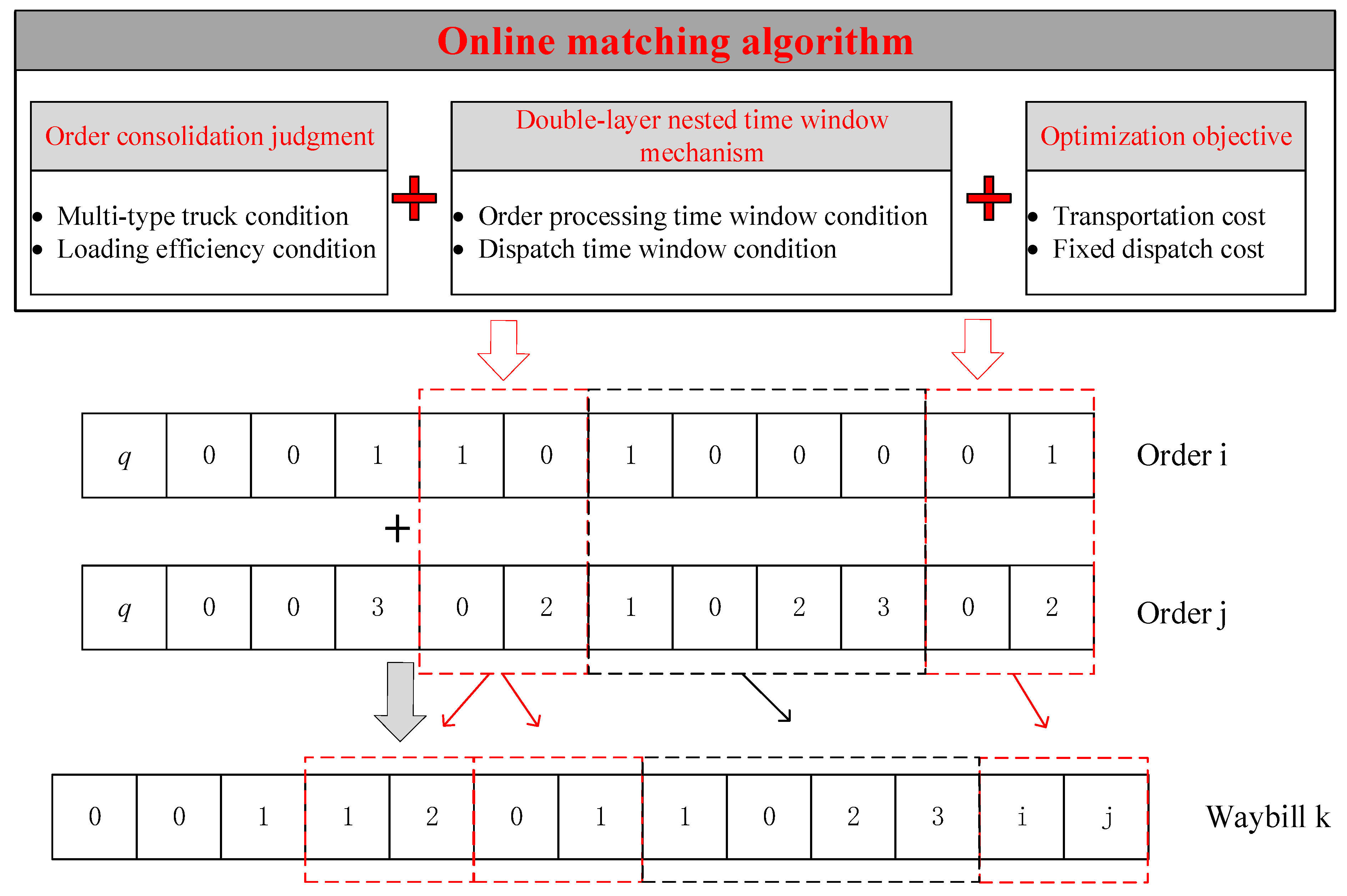
The order coding is based on the order information and consists of five parts, including the order type, order sequence number, cargo volume, order generation time, and node number. These are the basic pieces of information needed to make a matching decision. The pickup order numbered 1 generated by node 1 is shown in Figure 4, with cargo volume of 10 unitized units and the order generation time of 10:23.

4.1.2. Decoding Strategy

The coded orders input the algorithm in sequential order of generation time. Participate in the algorithmic judgment of the order list and conduct real-time online optimization under certain judgment conditions. Output the optimized waybills when successful matching and the corresponding orders are removed from the order list. The number of orders in the order list is time-varying. The consideration of a heterogeneous truck fleet with multiple truck types and widely distributed cooperative pickup nodes complicates the order consolidation judgment process of the online matching algorithm. The order–waybill decoding process is shown in Figure 5.
The online matching algorithm is optimized to output coded waybills. The sequential autogenerated waybill number, the type of truck assigned, the amount of cargo loaded on the truck, the waybill generation time, the truck visit route, and order service sequence for this truck are available. The waybill numbered 1 is shown in Figure 6, a truck of type 1 is assigned for transportation with a loaded cargo volume of 12 unitized units and the waybill generation time of 10:23. Truck service sequence is optimized with total costs as the optimization objective, and the service sequence for this example waybill starts from the core hub, then service order 2, order 3, and order 1 sequentially, and finally the return to the core hub. Due to the different number of orders served by the assigned trucks, the length of the waybill coding is uncertain. Furthermore, other parameters such as the loading efficiency of the trucks are also available.

4.2. The Solution Process of the Online Matching Algorithm

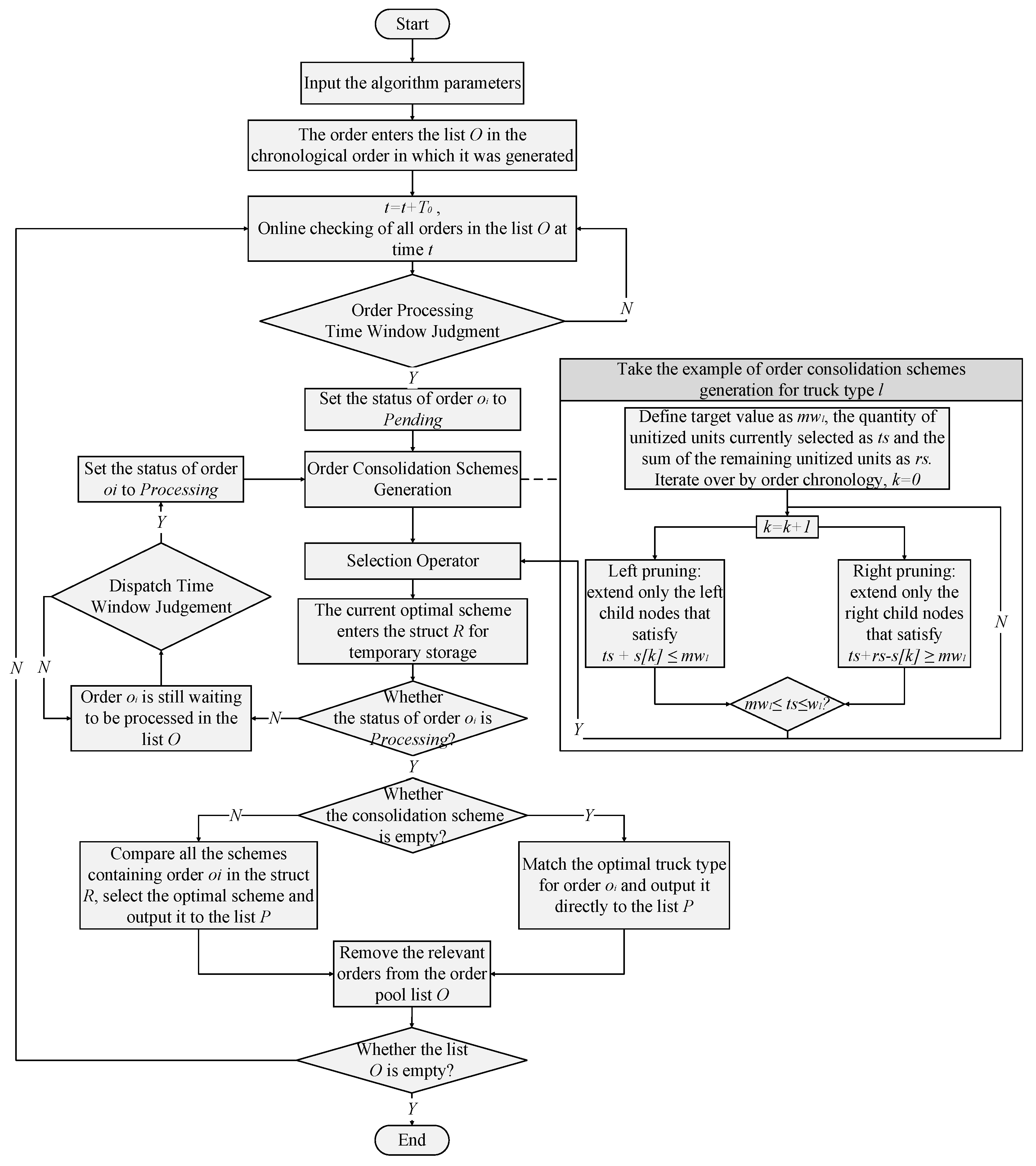
Online matching algorithm implements the truck–cargo matching and truck service sequence planning in the order list. The process of the algorithm is as follows (Algorithm 1):
Algorithm 1: Online Matching Algorithm
INPUT: Create list of orders O , struct of trucks to be dispatched R , list of waybills P , set of truck types L = { 1 , 2 , m } . Define the r t h generated order as o r , the number of unitized units for order o r as a r , and the pickup node number for order o r as s r . Define the loading efficiency condition for each truck as m .
STEP 1: Orders generated by different cooperative pickup nodes enter list O in chronological sequence.
STEP 2: Order Processing Time Window Judgment. Check all orders in list O at regular online checking interval T 0 . Checks whether there is an order o r in the current order list O that has reached the order processing time window T 1 and, if so, sets the status of the order o r to Pending.
STEP 3: Order consolidation schemes generation. Generates all consolidation schemes that satisfy the loading efficiency condition for each truck type.The specific judgment process: Determine whether there are a certain number of orders in the current list O with the quantity of unitized units can exactly satisfy the loading efficiency condition of each truck type, i.e., m × Q l a r + k r j a k Q l .
STEP 4: Selection Operator. Using total costs as an objective to select the optimal consolidation scheme.
The specific selection process: Obtain the lowest total cost of truck service sequence for all feasible schemes, including the truck transportation cost to service all orders in the scheme and the fixed dispatch cost for using such a type of truck. Temporarily store the optimal consolidation scheme (including related orders, the lowest total costs, truck service sequence, etc.) for pending order o r to the struct R .
STEP 5: Dispatch Time Window Judgment. Allow the order with successful consolidation to wait in the order list for T 2 mins for a better solution. If, at the moment of the regular online check, there is an order o r in list O that has reached the dispatch time window T 2 , the order o r must be processed at that moment. Sets the status of the order o r to Processing.
Repeat STEP 3 and STEP 4 to temporarily store the optimal consolidation scheme for the order o r under processing to the struct R . Compare all consolidation schemes related to order o r in struct R , select the one with the lowest total cost and output it to the waybill list P . Removes all the related orders from the list O .
STEP 6: Repeat the above steps until all the orders are processed, then end the algorithm. All the orders are in the list P , and order list O is empty.
In the online matching algorithm process, the backtracking method was used in the order consolidation judgment process for STEP 3, to obtain all feasible consolidation schemes, that is, the solution space tree of the problem is searched using a depth-first strategy. The search starts from the root node, and when a node is searched, a pruning function is used to determine if the node is feasible. If it is not feasible, skip searching the subtree and backtrack to its ancestor node; otherwise, enter the subtree to continue the search. This is as shown in Figure 7.
During the order accumulation process of the algorithm, each round of matching in the order list is an optimization process for all pending orders. The online matching algorithm designed in the study innovatively sets up a double-layer nested time window judgment mechanism to increase the solution space of the search and increase the possibility of better solutions.

5. Experiments and Data Analysis

5.1. Small Numerical Case

We evaluate the correctness of the proposed model and the effectiveness of the designed online matching algorithm through computational experiments performed on randomly generated order data sets as small numerical cases.

5.1.1. Input Data

(1) Order Data
The order data of small numerical cases include 14 pickup orders generated by 4 cooperative pickup nodes. The specific information about the orders generated by each node is shown in Table 5. The distribution of all the nodes and the distances between the nodes are shown in Appendix A.1.
(2) Truck and Unitized Implement Parameters
Order demand at different cooperative pickup nodes is uncertain, and the order demand at the same node but at different times is similarly uncertain. In addition to the different location distribution of different nodes, the type, volume, and weight of the shipment cargoes demanded by the pickup nodes are also different. Therefore, multiple types of trucks are usually configured to achieve flexible and efficient scheduling.
The numerical experiments consider 3 types of trucks and 2 types of unitized implements, with the specific parameters shown in Appendix A.2. The matching relationship between the different types of trucks and the unitized units are shown in Appendix A.3.
The other parameters used in the algorithm are listed in Table 6.

5.1.2. Results Analysis

(1) Optimization Scheme Analysis
The proposed online matching algorithm is used to solve the small numerical case and programmed by applying MATLAB™ 2018a. The details of the cost-optimal truck–cargo matching and truck scheduling scheme are shown in Table 7. The time window parameters are set as follows: the order processing time window T 1 is set to 20 min, and the scheduling time window T 2 is set to 1.25 min.
In addition, to validate the accuracy of the constructed model and the effectiveness of the designed algorithm, PyCharm platform is used to code Python 3.9 to call commercial solver Gurobi 9.5 to solve the mixed-integer nonlinear programming and set the termination condition as Gap reaches 1% or the computing time reaches 1 h. The details of the cost-optimal scheme are shown in Table 7. The order processing time window T 1 is set to 20 min.
The total cost of the optimal scheme obtained by calling the Gurobi solver is RMB 1302, and the total cost of the optimal scheme obtained by applying the online matching algorithm with reasonable algorithmic parameter settings is RMB 1337.2, with an optimality gap of 2.7%. In the comparison of the two optimized schemes, each generates three waybills, assigning the largest type of truck. The average load efficiency is the same, but the cost varies due to the different orders served.
The use of the Gurobi solver is to optimize according to the complete order information and obtain the global optimal result. In contrast, the online matching algorithm proposed in this paper makes optimization judgments based on partial order information at the current moment, which can only attain local optimal results. Therefore, this cost differential is acceptable. Meanwhile, since the Gurobi solver requires the input of complete information and cannot handle real-time demand, the optimization results will be output at the same time. There is no guarantee that the orders that are generated first will be prioritized to be served. The algorithm designed in this paper can be better adapted to the status of gradual order release in LTL logistics operation scenarios.
(2) Comparative analysis of results
Since the order information of the experiment is released gradually, the online matching algorithm can only utilize the currently known information for decision-making at any moment. Moreover, according to the realistic scenario, we stipulate that the decision made cannot be changed again. In general, there is no optimal online algorithm, and the algorithm parameters are adjusted to obtain better results.
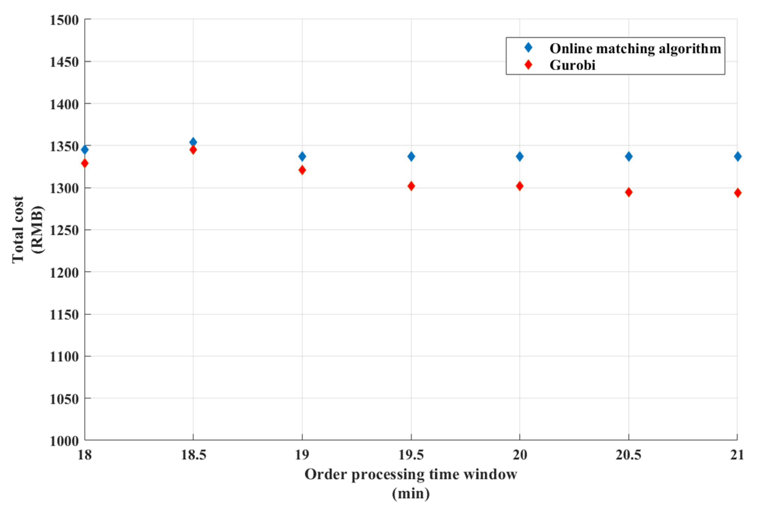
Adjust the parameters of the time window T 1 . Set the order processing time window to range from 18 to 21 min in 0.5 min steps. The result of the Gurobi solver is compared as an optimization upper bound. The results of different optimization schemes are shown in Table 8 and Figure 8. The average order waiting time is expressed as AWT.
The red rhombus in Figure 8 represents the optimal solution of Gurobi. In contrast, if the online matching algorithm is subjected to reasonable parameter settings, the optimization results with a smaller gap can be obtained. Overall, a shorter time window leads to more truck trips and lower average loading efficiency, resulting in increased costs. This is because there are a certain number of orders that have to be output without waiting for other orders to jointly consolidate a better scheme, so the higher the frequency of departure is not always the better. In addition, due to the high model complexity, comparing with the designed algorithms, using Gurobi to solve the small numerical case increases the algorithmic runtime exponentially, although a lower cost-optimal solution can be obtained. It is not able to handle larger-scale empirical cases efficiently.
Validating the dynamic response of the algorithm to real-time demands. Randomize the sequence of order generation to form 5 sets of order data and apply the online matching algorithm to solve. The optimization schemes are compared with the results of the Gurobi and online matching algorithms solving for the original order data input, as shown in Table 9. The time window parameter settings are consistent with scheme 1.
From the previous section, different order generation sequences will have no effect on the result of the Gurobi solver. However, from the schemes in Table 9, it slightly affects the solution results of the online matching algorithm. It shows that the algorithm is responsive to changes in order demand.

5.2. Empirical Case

The empirical case is numerically performed using real business data from the Shunhe IOT LTL logistics hub in Linyi, Shandong Province, China.

5.2.1. Input Data

(1) Order Data
The order data include 200 pickup orders generated by 7 cooperative pickup nodes distributed in Linyi city, with order generation time from 8:00 to 14:30. The shipment cargoes cover more than twenty categories, including electronic devices, furniture, cosmetics, clothing, food, and pharmaceuticals, etc. They are packaged in bags or boxes, and unitized implements such as pallets or assembly cages are often used for loading, assembled into a unitized unit. When a waybill is generated, the appropriate type of pickup truck needs to be assigned to pick up the cargoes from the corresponding pickup nodes in sequence.
The distribution of all the nodes and the distances between the nodes are shown in Figure 9 and Appendix A.1.
(2) Other Parameters
The truck and unitized implement parameters and the time window parameters used are the same as for the small numerical case.

5.2.2. Results Analysis

Based on the input data and the designed online matching algorithm, the waybills are generated. Assign a matching type of truck to the waybill and rationalize the sequence of truck services. Achieve the truck–cargo matching and pickup truck scheduling schemes.
(1) Optimization Scheme Analysis
Details of the cost-optimal truck–cargo matching and truck scheduling scheme are shown in Table 10. The time window parameters are set as follows: the order processing time window T 1 is set to 20.5 min, and the scheduling time window T 2 is set to 1.25 min.
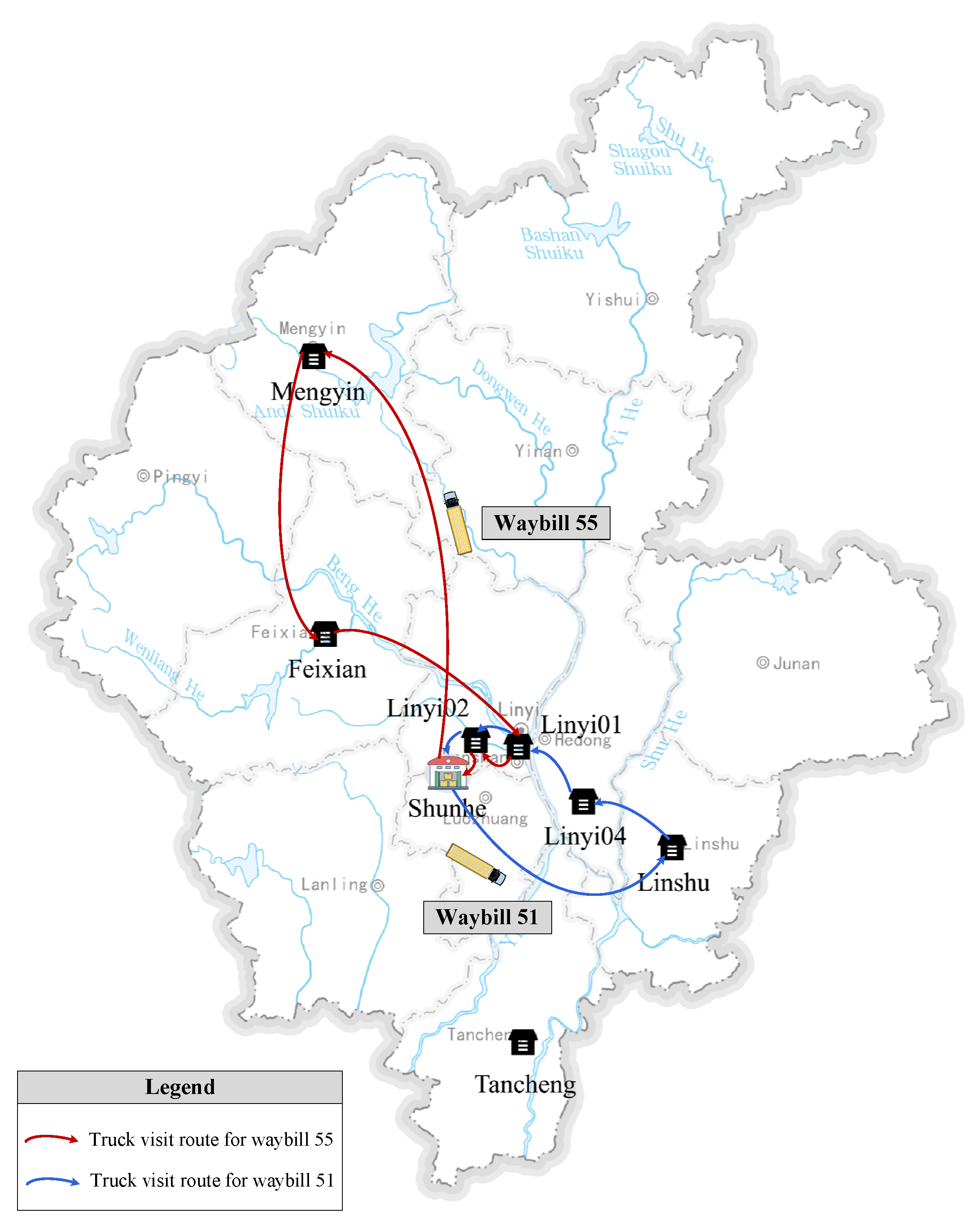
The total cost of the optimal scheme is RMB 65,195, and a total of 59 truck trips were generated, with truck type III accounting for 83%. The average loading efficiency of all the waybills is close to 95%. The optimal solution has more multi-node pickup waybills to increase the load efficiency and reduce the average cost, with a share of 65.5%. A maximum of four pickup nodes visited for each truck, and the truck routes for waybill 51 and waybill 55 are shown in Figure 10. The service area of each truck is reasonable, and there is no significant detour across a wide range of areas, such as visiting Mengyin and Tancheng in turn.
(2) Comparative Analysis of Results
Since the order information of the experiment is released gradually, the online matching algorithm can only utilize the currently known information for decision-making at any moment. Moreover, according to the realistic scenario, we stipulate that the decision made cannot be changed again. In general, there is no optimal online algorithm, and the algorithm parameters are adjusted to obtain better results.
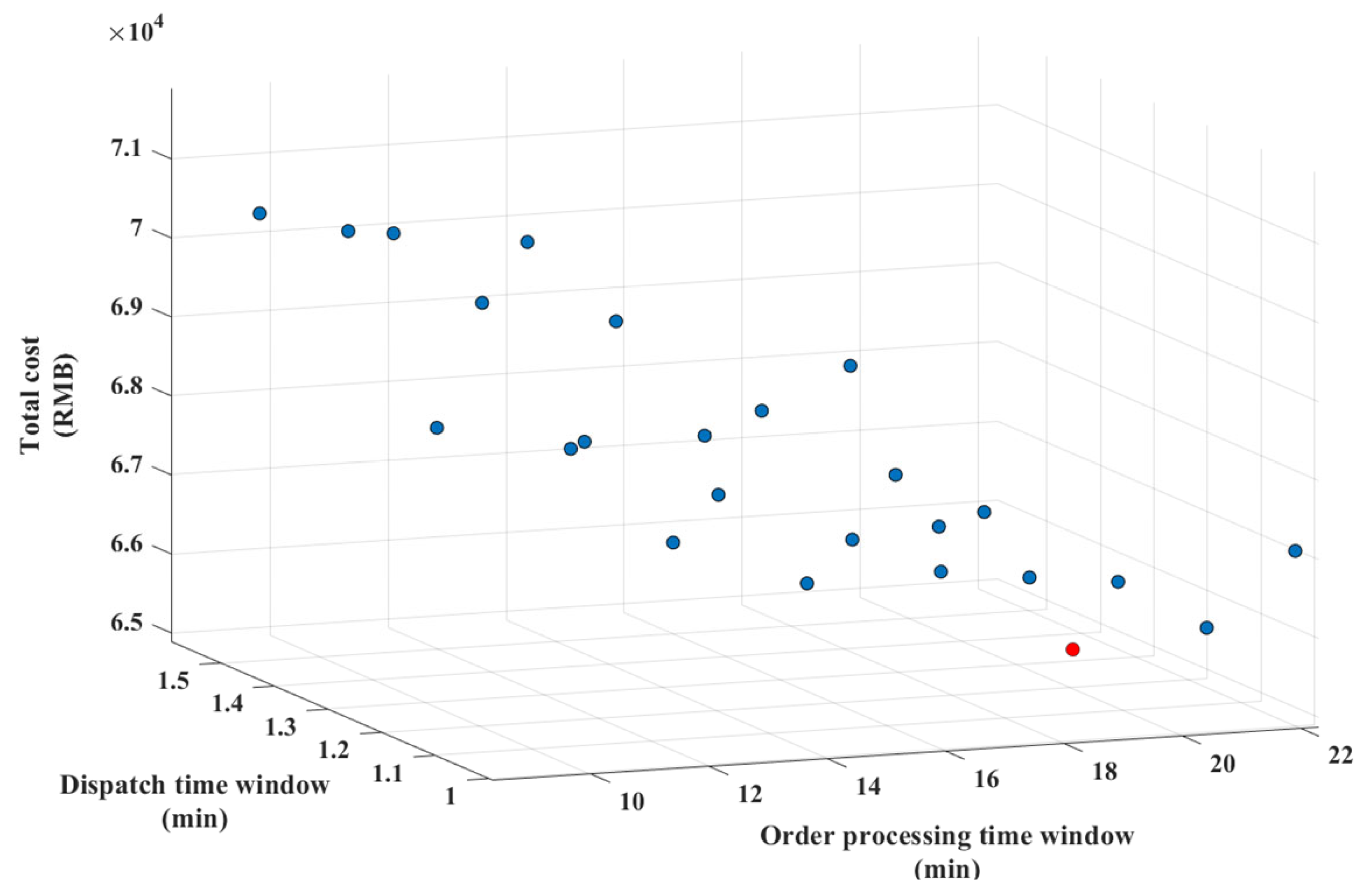
Adjust the parameters of the double-layer nested time window. Set the order processing time window to range from 9 to 22 min in 1.5 min steps, and set the dispatch time window to range from 1 to 1.5 min in quarter-minute steps. The results of different optimization schemes are shown in Table 11 and Figure 11.
The red dot in Figure 11 represents the optimal solution. The total cost of the optimal scheme 23 is nearly 10% lower compared to the highest cost scheme. Overall, setting longer time windows, while causing orders to wait longer in the order list, results in better optimization, reflected in lower total cost and fewer truck trips. In particular, by increasing the number of larger types of trucks, the number of smaller types of trucks has been significantly reduced, resulting in lower average costs. However, a longer time window is not necessarily better. Scheme 24 has a longer dispatch time window, and scheme 25 has a longer order processing time window compared to scheme 23, which bring about a reduction in the number of truck trips, but result in a higher total cost due to the truck serving more nodes and existing unnecessary detours.
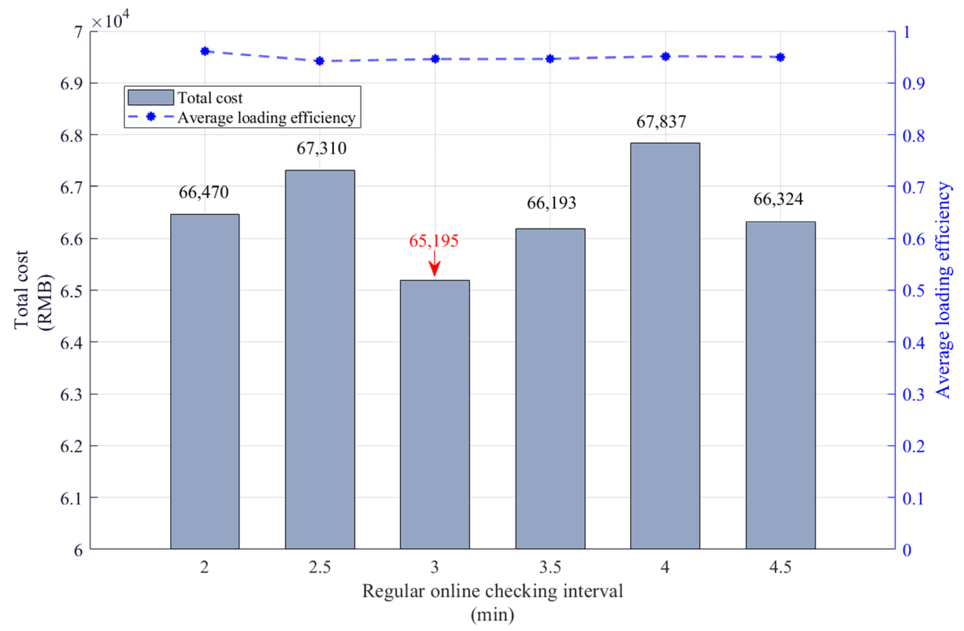
Adjust the parameters of the regular online checking interval. The checking interval should be set much shorter than the order processing time window to avoid orders that exceed the processing time window and are not being processed in time. However, too short an interval brings too high a check frequency, which is a waste of computing resources. Set the regular online checking interval to range from 2 to 4.5 min in 0.5 min steps. The results of different optimization schemes are shown in Table 12 and Figure 12.
Figure 12 shows that the fine-tuning of the regular online checking interval results in little change in the number of truck trips and truck loading efficiency but large fluctuations in total cost. In terms of cost objectives, appropriate selection of checking interval is conducive to obtaining lower total operating costs.
Furthermore, different algorithmic scenarios are considered. When the online matching algorithm is not used for optimization, generated orders must be processed instantly, and only the current order information is considered for the matching decision. Then, adjust the double-layer nested time window mechanism. When there is no time window, that is, the lengths of the double-layer time windows are both set to 0, it means that all generated orders in the current order list must be processed at each regular online checking time. When only a single time window is set, without considering the extra dispatch time window, the order processing time window is set to 20.5 min. The results for the different scenarios and the comparison with the optimal schemes are shown in Table 13.
In summary, the optimization of order consolidation using the designed online matching algorithm is significant and justifies the necessity of time window settings. In particular, the better optimization results are obtained due to the setup of the double-layer nested time window mechanism. It reduces the use of smaller trucks by increasing the number of trips by truck type III. As a result, fixed dispatch costs and variable transportation costs are reduced, bringing about a 3.8% reduction in total costs and a 1.24% increase in average loading efficiency compared to the single time window setting.
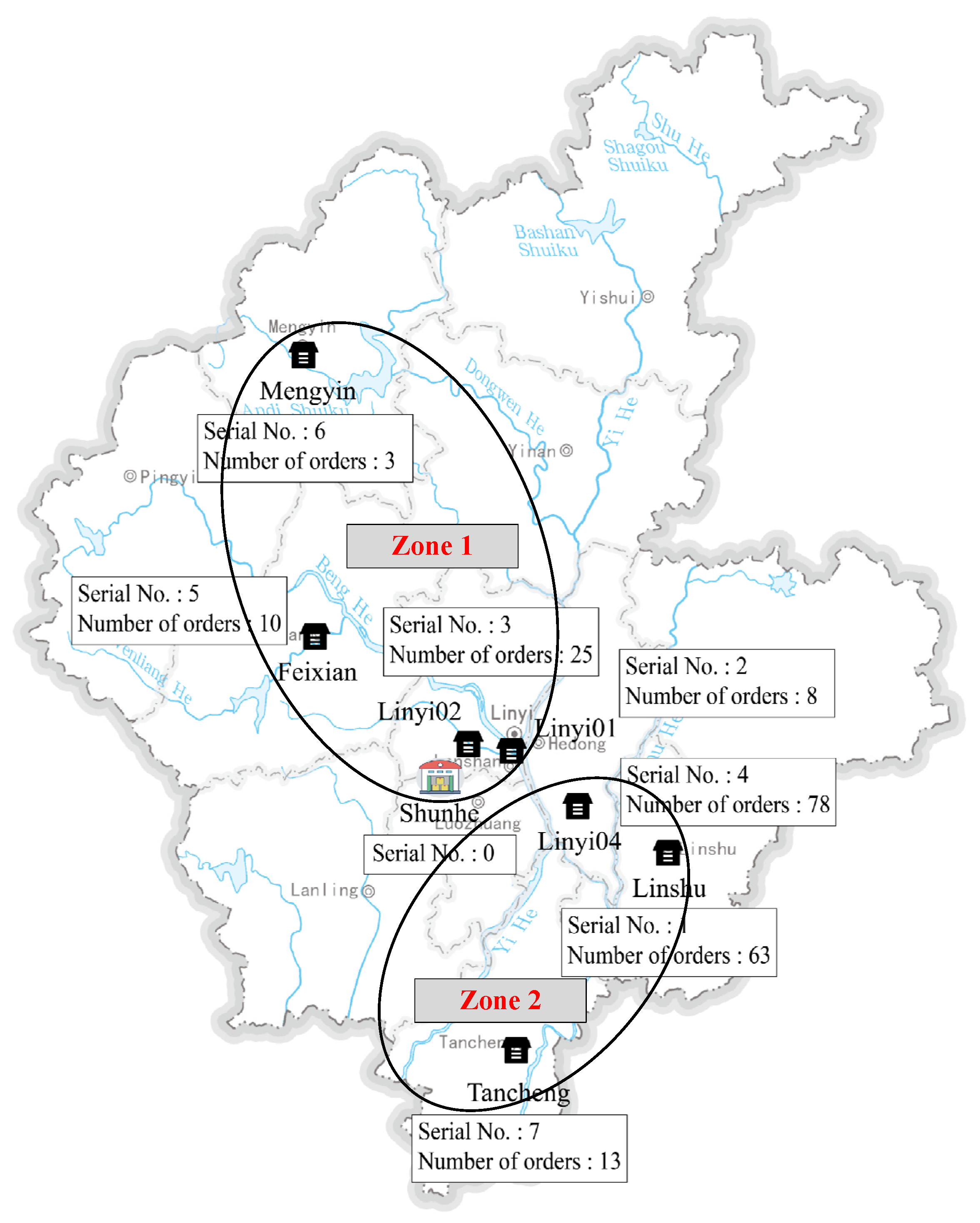
Consider service zone partitioning. As an example, a service zone partitioning approach is applied by dividing the pickup nodes into two zones according to their geographic location (considering north and south of the Shunhe hub), as shown in Figure 13. The online matching algorithm is used to solve respectively, and the optimal schemes are obtained as shown in Table 14 and Table 15. The parameters used are the same as for the empirical case.
The total cost of the optimal scheme with service zone partitioning to accomplish the LTL pickup assignment is RMB 65,636, which is a 0.7% increase in cost compared to the case without partitioning. The waybills of the three types of trucks accounted for 16.5%, 24.5%, and 60%, respectively, which mainly increased the number of trips for truck types I and II. This is because if there is no zone partitioning, some neighboring nodes to the north of the hub can also carry out mixed transportation with nodes to the south, to improve load efficiency and reduce the number of trucks used. Although it may lead to increased transportation costs, it can significantly reduce the dispatch cost, thus achieving a reduction in the total cost. Meanwhile, the algorithm designed in this paper is cost-oriented for optimization, so the high cost caused by unreasonable detours is not allowed in the optimal scheme.

5.3. Managerial Insights

Currently, the LTL logistics market is huge with a large number of market participants. However, the LTL logistics market is highly fragmented, and the allocation of logistics resources is unreasonable and insufficient. From the results of the case studies in this paper, it is clear that the integration of LTL logistics information resources, rational truck–cargo matching optimization, and coordinated scheduling of capacity resources can effectively reduce the operating costs of LTL logistics hubs.
Therefore, we suggest that LTL hubs establish logistics information platforms, integrate order demands information, and apply efficient algorithms to realize efficient truck–cargo matching and vehicle scheduling. Promote the transformation of digitalization and intelligence in LTL logistics. Thus, it enables rapid response to real-time demand, truck–cargo matching and truck scheduling, reduces operational costs through scale economy, and provides a guarantee for the efficient and stable business operation of the LTL hub operators.

6. Conclusions

Rapid economic development and the upgrading of people’s consumption patterns have driven the rapid development of LTL logistics and put forward higher requirements for the quick response to LTL logistics demand. There is an urgent need for LTL operators to apply optimization technology for reasonable and sufficient resource allocation.
In this study, based on analyzing the characteristics of LTL logistics order data, the scientific problem is abstracted. With the objective of minimizing the operation cost, the LTL truck–cargo matching and truck scheduling model is constructed, and the online matching optimization algorithm considering real-time scheduling is designed to solve the problem. It is demonstrated that the model and algorithm have great effectiveness and efficiency, based on a randomly generated small numerical case, and compared with the optimal results solved by Gurobi. By inputting the real business data for simulation and measurement and analyzing the results, the results of the study showed that the optimal scheme reaches a truck loading efficiency of nearly 95% by reasonably setting the algorithm parameters. Compared with the scenario without order consolidation, the number of trips is reduced by 71%, and the total cost is reduced by 38.8%. In addition, the setting of the double-layer nested time window mechanism performs well for optimization. The total costs are reduced by 34% and 3.8% compared to no time window and single time window setting, respectively. Moreover, a comparison is made between restricted pickup operations conducted on the basis of zone partitioning. The results show that for this problem, zoning does not lead to better optimization results.
However, our study simplifies the matching relationship between the cargo and the unitized implements. In the future, we will refer to related studies [23,24,28] to further refine the unitized implement–order–cargo matching relationship and enrich the existing research by studying the truck–cargo matching and truck scheduling problem based on the three-dimensional loading of multiple types of LTL cargoes and unitized implements.

Author Contributions

Conceptualization, W.T. and X.C.; Methodology, W.T. and X.C.; Validation, X.C.; Formal analysis, W.T.; Investigation, S.L., Y.L. and W.L.; Resources, M.L.; Writing—original draft, W.T.; Writing—review & editing, X.C. and M.L.; Supervision, M.L. All authors have read and agreed to the published version of the manuscript.

Funding

This research is funded by the National Key Research and Development Program of China (2021YFB1407003).

Data Availability Statement

Data are contained within the article.

Conflicts of Interest

The authors declare no conflicts of interest.

Appendix A

Appendix A.1. The Distances between the Nodes

Table A1. Distance between each node in small numerical case (Unit: kilometers).
Node 0Node 1Node 2Node 3Node 4
Node 004633
Node 140367
Node 263023
Node 336202
Node 437320
Table A2. Distance between each node in empirical case (Unit: kilometers).
Node 0Node 1Node 2Node 3Node 4Node 5Node 6Node 7
Node 00508530358674
Node 15004045209015055
Node 28400322388470
Node 35453025408075
Node 43020222506011050
Node 53590384060060104
Node 6861508480110600152
Node 774557075501041520

Appendix A.2. Truck and Unitized Implement Parameters

Table A3. Parameters of the truck type.
Truck TypeLoading Length
(m)
Loading Width
(m)
Weight Capacity
(t)
Number of Unitized Units Can Be Loaded
(pcs)
Unit Dispatch Cost
(RMB/trip)
Unit Transportation Cost
(RMB/pcs·km)
Type I4.22.1527122800.35
Type II6.82.4556203000.30
Type III122.4581443400.20
Table A4. Parameters of the unitized implements.
Unitized Implement TypeLength (m)Width (m)Height (m)
Assembly cage1.210.89
Pallet1.210.15

Appendix A.3. The Matching Relationship between the Different Types of Trucks and the Unitized Units
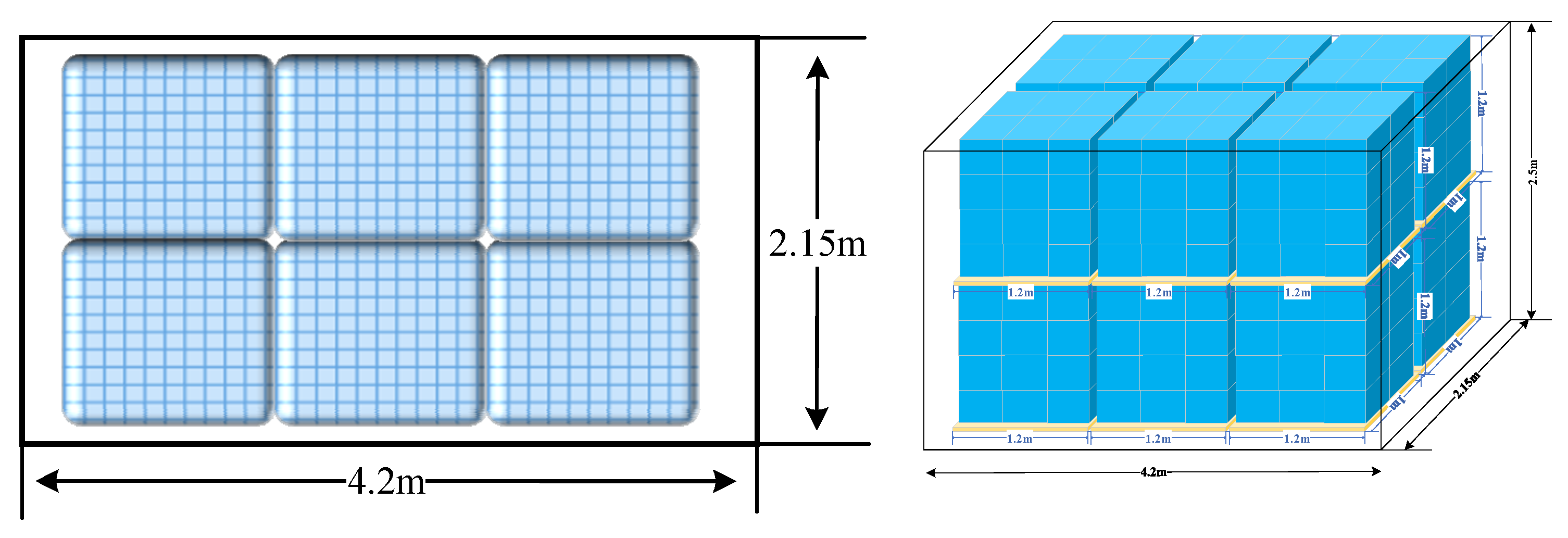
Figure A1. Schematic loading of unitized units for pickup trucks of type I (planar/dimensional).
Mathematics 12 00755 g0a1
Figure A2. Schematic loading of unitized units for pickup trucks of type II (planar/dimensional).
Mathematics 12 00755 g0a2
Figure A3. Schematic loading of unitized units for pickup trucks of type III (planar/dimensional).
Mathematics 12 00755 g0a3

References

  1. Forkenbrock, D. Comparison of external costs of rail and truck freight transportation. Transp. Res. Part A Policy Pract. 2001, 35, 321–337. [Google Scholar] [CrossRef]
  2. Ni, L.; Wang, X. Load factors of less-than-truckload delivery tours: An analysis with operation data. Transp. Res. Part E Logist. Transp. Rev. 2021, 150, 102296. [Google Scholar] [CrossRef]
  3. Tan, K.; Xu, F.; Fang, X.; Li, C. Research on Location Selection for Urban Networks of Less-than-Truckload Express Enterprises Based on Improved Immune Optimization Algorithm. Mathematics 2023, 11, 1543. [Google Scholar] [CrossRef]
  4. Herszterg, I.; Ridouane, Y.; Boland, N.; Erera, A.; Savelsbergh, M. Near real-time loadplan adjustments for less-than-truckload carriers. Eur. J. Oper. Res. 2022, 301, 1021–1034. [Google Scholar] [CrossRef]
  5. Ahmad, B.; Natashia, B.; Martin, S. The Dynamic Freight Routing Problem for Less-Than-Truckload Carriers. Transp. Sci. 2022, 57, 717–740. [Google Scholar]
  6. Giovanni, L.; Gastaldon, N.; Losego, M.; Sottovia, F. Algorithms for a Vehicle Routing Tool Supporting Express Freight Delivery in Small Trucking Companies. Transp. Res. Procedia 2018, 30, 197–206. [Google Scholar] [CrossRef]
  7. Shi, H.; Sun, L.; Teng, Y.; Hu, X. An online intelligent vehicle routing and scheduling approach for B2C e-commerce urban logistics distribution. Procedia Comput. Sci. 2019, 159, 2533–2542. [Google Scholar] [CrossRef]
  8. Cantarella, G.; Fiori, C. Multi-vehicle assignment with elastic vehicle choice behaviour: Fixed-point, deterministic process and stochastic process models. Transp. Res. Part C Emerg. Technol. 2022, 134, 103429. [Google Scholar] [CrossRef]
  9. Wang, Y.; Wei, Y.; Wang, X.; Wang, Z.; Wang, H. A clustering-based extended genetic algorithm for the multidepot vehicle routing problem with time windows and three-dimensional loading constraints. Appl. Soft Comput. 2023, 133, 109922. [Google Scholar] [CrossRef]
  10. Pasha, J.; Li, B.; Elmi, Z.; Fathollahi-Fard, A.; Lau, Y.; Roshani, A.; Kawasaki, T.; Dulebenets, M. Electric vehicle scheduling: State of the art, critical challenges, and future research opportunities. J. Ind. Inf. Integr. 2024, 38, 100561. [Google Scholar] [CrossRef]
  11. Ouyang, Z.; Leung, E.; Huang, G. Community logistics for dynamic vehicle dispatching: The effects of community departure “time” and “space”. Transp. Res. Part E Logist. Transp. Rev. 2022, 165, 102842. [Google Scholar] [CrossRef]
  12. Diefenbach, H.; Emde, S.; Glock, C. Multi-depot electric vehicle scheduling in in-plant production logistics considering non-linear charging models. Eur. J. Oper. Res. 2023, 306, 828–848. [Google Scholar] [CrossRef]
  13. Low, C.; Chang, C.; Li, R.; Huang, C. Coordination of production scheduling and delivery problems with heterogeneous fleet. Int. J. Prod. Econ. 2014, 153, 139–148. [Google Scholar] [CrossRef]
  14. Wang, J.; Yao, S.; Sheng, J.; Yang, H. Minimizing total carbon emissions in an integrated machine scheduling and vehicle routing problem. J. Clean. Prod. 2019, 229, 1004–1017. [Google Scholar] [CrossRef]
  15. Fathollahi-Fard, A.; Woodward, L.; Akhrif, O. Sustainable distributed permutation flow-shop scheduling model based on a triple bottom line concept. J. Ind. Inf. Integr. 2021, 24, 100233. [Google Scholar] [CrossRef]
  16. Ganji, M.; Kazemipoor, H.; Molana, M.; Sajadi, S. A green multi-objective integrated scheduling of production and distribution with heterogeneous fleet vehicle routing and time windows. J. Clean. Prod. 2020, 259, 120824. [Google Scholar] [CrossRef]
  17. Yağmur, E.; Kesen, S. Multi-trip heterogeneous vehicle routing problem coordinated with production scheduling: Memetic algorithm and simulated annealing approaches. Comput. Ind. Eng. 2021, 161, 107649. [Google Scholar] [CrossRef]
  18. Kang, Y.; Lee, S.; Chung, B. Learning-based logistics planning and scheduling for crowdsourced parcel delivery. Comput. Ind. Eng. 2019, 132, 271–279. [Google Scholar] [CrossRef]
  19. Wehbi, L.; Bektaş, T.; Iris, C. Optimising vehicle and on-foot porter routing in urban logistics. Transp. Res. Part D Transp. Environ. 2022, 109, 103371. [Google Scholar] [CrossRef]
  20. Gu, R.; Liu, Y.; Poon, M. Dynamic truck–drone routing problem for scheduled deliveries and on-demand pickups with time-related constraints. Transp. Res. Part C Emerg. Technol. 2023, 151, 104139. [Google Scholar] [CrossRef]
  21. Tian, R.; Wang, C.; Ma, Z.; Liu, Y.; Gao, S. Research on vehicle-cargo matching algorithm based on improved dynamic Bayesian network. Comput. Ind. Eng. 2022, 168, 108039. [Google Scholar] [CrossRef]
  22. Yu, X.; Huang, D.; Gao, Y.; Zhu, J.; Ren, B. Research on Vehicle and Cargo Matching of Electric Materials Based on Weed Optimization Algorithm. Lect. Notes Electr. Eng. 2023, 996, 380–388. [Google Scholar]
  23. Wang, N.; Zhang, J.; Zhao, J. Vehicle Routing Problem of Intercity Transportation Platform for Less-than-truck-load Cargo. J. Transp. Syst. Eng. Inf. Technol. 2022, 22, 163–177. [Google Scholar]
  24. Yücel, E.; Salman, F.; Erdoğan, G. Optimizing two-dimensional vehicle loading and dispatching decisions in freight logistics. Eur. J. Oper. Res. 2022, 102, 954–969. [Google Scholar] [CrossRef]
  25. Li, J.; Zheng, Y.; Dai, B.; Yu, J. Implications of matching and pricing strategies for multiple-delivery-points service in a freight O2O platform. Transp. Res. Part E Logist. Transp. Rev. 2020, 136, 101871. [Google Scholar] [CrossRef]
  26. Ni, S.; Luo, X.; Xiao, B. Optimization of Vehicle–Cargo Matching Regarding Interests of Three Parties. J. Southwest. Jiaotong Univ. 2023, 58, 48–57. [Google Scholar]
  27. Deng, J.; Chen, X.; Wei, W.; Liang, J. Resource coordination scheduling optimisation of logistics information sharing platform considering decision response and competition. Comput. Ind. Eng. 2023, 176, 108892. [Google Scholar] [CrossRef]
  28. Iris, C.; Christensen, J.; Pacino, D.; Ropke, S. Flexible ship loading problem with transfer vehicle assignment and scheduling. Transp. Res. Part B Methodol. 2018, 111, 113–134. [Google Scholar] [CrossRef]
  29. Agatz, N.; Erera, A.; Savelsbergh, M.; Wang, X. Optimization for dynamic ride-sharing: A review. Eur. J. Oper. Res. 2012, 223, 295–303. [Google Scholar] [CrossRef]
  30. Guo, X.; Caros, N.; Zhao, J. Robust matching-integrated vehicle rebalancing in ride-hailing system with uncertain demand. Transp. Res. Part B Methodol. 2021, 150, 161–189. [Google Scholar] [CrossRef]
  31. Zhan, X.; Szeto, W.; Chen, X. The dynamic ride-hailing sharing problem with multiple vehicle types and user classes. Transp. Res. Part E Logist. Transp. Rev. 2022, 168, 102891. [Google Scholar] [CrossRef]
  32. Meshkani, S.; Farooq, B. Centralized and decentralized algorithms for two-to-one matching problem in ridehailing systems. EURO J. Transp. Logist. 2023, 12, 100106. [Google Scholar] [CrossRef]
  33. Zhou, Z.; Roncoli, C. A scalable vehicle assignment and routing strategy for real-time on-demand ridesharing considering endogenous congestion. Transp. Res. Part C Emerg. Technol. 2022, 139, 103658. [Google Scholar] [CrossRef]
  34. Qin, X.; Yang, H.; Wu, Y.; Zhu, H. Multi-party ride-matching problem in the ride-hailing market with bundled option services. Transp. Res. Part C Emerg. Technol. 2021, 131, 103287. [Google Scholar] [CrossRef]
  35. Albers, S. Online algorithms: A survey. Math. Program. 2003, 97, 3–26. [Google Scholar] [CrossRef]
  36. Park, H.; Waddell, D.; Haghani, A. Online optimization with look-ahead for freeway emergency vehicle dispatching considering availability. Transp. Res. Part C Emerg. Technol. 2019, 109, 95–116. [Google Scholar] [CrossRef]
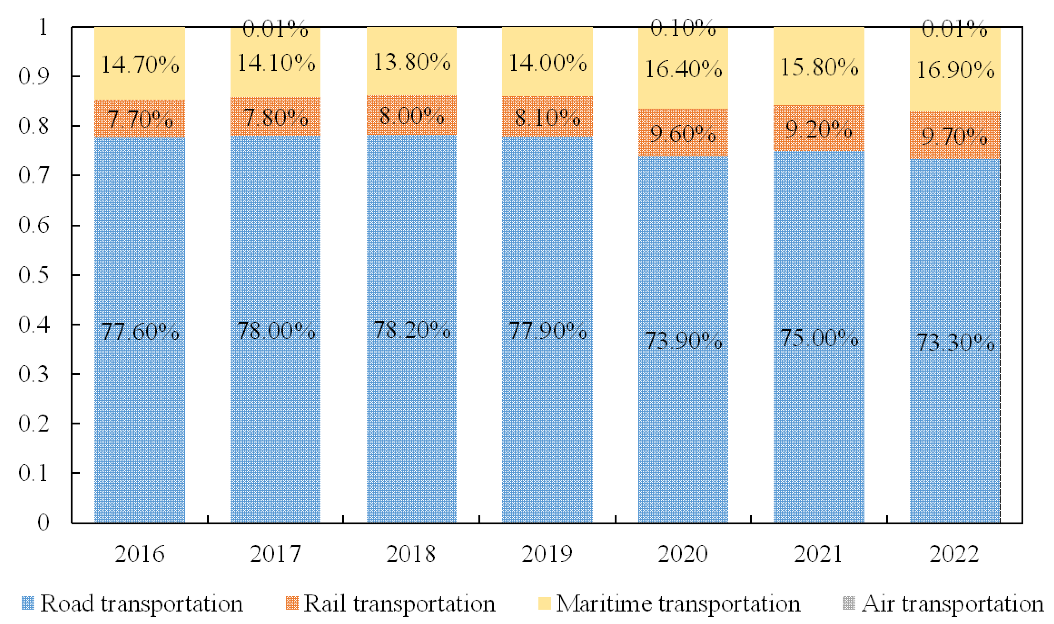
Figure 1. Percentage of four modes of freight transportation in China, 2016–2022.
Mathematics 12 00755 g001
Figure 2. Schematic of the LTL truck–cargo matching problem.
Mathematics 12 00755 g002
Figure 3. Schematic of truck–cargo matching process.
Mathematics 12 00755 g003
Figure 4. Example of order coding.
Mathematics 12 00755 g004
Figure 5. The order–waybill decoding process.
Mathematics 12 00755 g005
Figure 6. Example of waybills coding.
Mathematics 12 00755 g006
Figure 7. Flowchart of online matching algorithm.
Mathematics 12 00755 g007
Figure 8. Results of the optimization schemes (small numerical case).
Mathematics 12 00755 g008
Figure 9. Distribution of nodes.
Mathematics 12 00755 g009
Figure 10. Truck visit route for waybill 51 and waybill 55.
Mathematics 12 00755 g010
Figure 11. Results of the optimization schemes (empirical case).
Mathematics 12 00755 g011
Figure 12. Sensitivity analysis of regular online checking interval (empirical case).
Mathematics 12 00755 g012
Figure 13. Service zone partitioning.
Mathematics 12 00755 g013
Table 1. Three main modes of transport in the road freight logistics industry.
ModeExpressLTL LogisticsFTL Logistics
Target marketC2C, B2CB2BB2B
Shipment weight<30 kg30 kg~3 t>3 t
Market concentrationhighcomparatively lowlow
Timeliness requirementhighcomparatively lowlow
Table 2. The main features of the previous relevant survey studies and our study (logistics vehicle scheduling problem).
Authors
(Year)
Application ScenarioModelObjectiveAlgorithm
Giovanni et al. [6]
(2018)
Express logistics--Neighborhood search heuristic algorithm
Shi et al. [7] (2019)B2C e-commerceInteger programming modelMinimize the number of feasible routes selectedOnline intelligent scheduling approach
Wang et al. [9] (2023)Bulky cargo logisticsMixed-integer programming modelMaximize the average loading rate of vehicles and minimize the total operating costsExtended nondominated sorting genetic algorithm-II
Diefenbach et al. [12] (2023)In-plant logisticsInteger programming modelMinimize the number of required vehiclesDecomposition scheme based on branch-and-check approach
Low et al. [13] (2014)Production scheduling with deliveryNonlinear programming modelMinimize the total costAdaptive genetic algorithm
Wang et al. [14]
(2019)
Machine schedulingNonlinear programming model Minimize the total carbon emissionsTabu search hybrid algorithm
Fathollahi-Fard et al. [15] (2021)Production schedulingMixed-integer linear programming modelMaximize the social benefitsLearning-based heuristic algorithm
Ganji et al. [16] (2020)Integrated scheduling of production and distributionMixed-integer nonlinear programming modelMinimize total distribution costs, carbon emission, and customer dissatisfactionNSGAII algorithm
Yagmur et al. [17]
(2021)
Integrated scheduling of production and distributionMixed-integer programming modelMinimize the sum of total tour time and total tardinessMemetic Algorithm
Kang et al. [18] (2019)Crowdsourced parcel delivery--Learning-based logistics planning and scheduling algorithm
Wehbi et al. [19]
(2022)
Urban delivery system Mixed-integer linear programming modelMinimize the total time of deliveryHeuristic algorithm
Gu et al. [20] (2023)Drone deliveryMarkov decision processMaximize the total profitsHeuristic solution approach framework
This studyLTL logisticsMixed-integer nonlinear programming modelMinimize the total costOnline matching algorithm
Table 3. The main features of the previous relevant survey studies and our study (vehicle–cargo matching problem).
Authors
(Year)
Freight TransportationPassenger TransportationStatic Matching ProblemDynamic Matching ProblemMulti-Type VehicleIntegrated Loading ProblemIntegrated Scheduling ProblemAlgorithm
Tian et al. [21] (2022) Improved dynamic Bayesian network
Yu et al. [22] (2023) Weed optimization algorithm
Wang et al. [23] (2022) Hybrid quantum particle swarm algorithm
Yücel et al. [24] (2022) ALNS algorithm
Li et al. [25] (2020) Heuristic-based algorithm
Ni et al. [26] (2023) NSGA II
Deng et al. [27] (2023) Particle swarm and genetic algorithm
Iris et al. [28] (2018) Randomized construction heuristic approach
Agatz et al. [29] (2012) _
Guo et al. [30] (2021) Robust optimization
Zhan et al. [31] (2023) Artificial bee colony algorithm
Meshkani et al. [32] (2023) Two-step ride-matching algorithm
Zhou et al. [33] (2022) Insertion heuristic method
Qin et al. [34] (2021) Two-stage KM-based approach
This study Future researchOnline Algorithm
Table 4. Model notations.
Set:
N = { 0 , 1 , 2 , n + 1 } Set of nodes, the total number of nodes is n + 2
{ 0 , n + 1 } N Core hub node set
N = { 1 , 2 , 3 n } N Cooperative pickup node set
J = J 1 J 2 J n Set of orders for n cooperative pickup nodes
L = { 1 , 2 , , m } Set of pickup truck types, the total number of truck types is m
K = K 1 K 2 K m Set of trucks
J l k Order set for truck k services
Parameters:
c l d i s p a t c h Fixed dispatch cost for truck type l
c l t r a n s Unit transportation cost of truck type l
d i j Transportation distance from node i to node j
Q l Capacity of truck type l
Q i a l k The total load of truck k of type l after serving order a generated by node i
q i a The quantity of unitized units for order a generated by node i
q i The number of orders generated by node i
T i a The generation time of order a generated by node i
T i a l k Time for truck k of type l to arrive at node i and ready to start serving order a
T 1 Order processing time window
Decision variables:
x i a l Binary variable, equal to 1 if the order a generated by node i is transported by a truck of type l , otherwise, equal to 0
w i a l k Binary variable, equal to 1 if the order a generated by node i is transported by truck k of type l , otherwise, equal to 0
z i l k Binary variable, equal to 1 if truck k of type l service node i , otherwise, equal to 0
y i a j b l k Binary variable, equal to 1 if the truck k of type l services order a generated by node i and followed by services order b generated by node j , otherwise, equal to 0
Table 5. Orders information.
Order Sequence NumberNode NumberCargo VolumeOrder Generation Time
1218:20:03
2398:27:33
3138:31:54
4118:33:27
52178:36:08
62138:37:33
72108:38:57
81138:39:11
94118:40:30
10358:42:33
11368:42:55
124178:47:39
131118:47:43
144128:49:12
Table 6. The other parameters.
ParametersDescriptionValue
m Truck loading efficiency requirement90%
T 0 Regular online checking interval3 min
Table 7. Optimal scheme waybill information (small numerical case).
AlgorithmWaybill No.Waybill Generation TimeNumber of Online CheckingTruck TypeCargo Volume
(pcs)
Cost
(RMB)
Loading EfficiencyTruck Service Sequence
i.e., →Node Number(Order Sequence Number)→
Online Matching Algorithm18:43:058344428100.00%0 → 3(2) → 3(10) → 2(6) → 2(7) → 2(1) → 3(11) → 0
28:54:3712344454.4100.00%0 → 1(3) → 1(4) → 2(5) → 4(9) → 4(14) → 0
39:03:1515341454.893.18%0 → 4(12) → 1(8) → 1(13) → 0
Gurobi18:47:46-341454.893.18%0 → 1(1) → 2(7) → 1(2) → 1(4) → 1(3) → 0
28:49:12-344410.4100.00%0 → 3(9) → 3(11) → 4(14) → 4(13) → 0
38:42:35-344436.8100.00%0 → 3(10) → 2(5) → 2(8) → 2(6) → 4(12) → 0
Table 8. Results of the optimization schemes (small numerical case).
Scheme No. T 1
(min)
Total Number of TripsTruck Type ITruck Type IITruck Type IIITotal Cost
(Algorithm)
(RMB)
Total Cost
(Gurobi)
(RMB)
Gap Algorithm Runtime
(Algorithm/Gurobi)
(s)
12130031337.21293.83.25%73.16/3159.36
220.530031337.21294.43.20%72.86/3150.9
32030031337.213022.63%36.75/3025.75
419.530031337.213022.63%37.34/2769.47
51930031337.21320.81.23%41.06/2896.25
618.530031353.61345.40.61%64.22/2078.93
71830031345.413291.22%22.01/1856.65
Table 9. Results of the optimization scheme for demand fluctuations (small numerical case).
Scheme No.Total Number of TripsTruck Type I Truck Type II Truck Type III Truck Cargo Volume
(pcs)
Average Loading EfficiencyAWT
(min)
Total Cost
(RMB)
Gap with
Gurobi
Algorithm Runtime
(s)
0
(Gurobi)
300344/44/4197.73%-1302-3025
1
(Original order data)
300344/44/4197.73%13.281337.22.70%342.051
2300343/43/4397.73%14.931329.62.12%279.595
3300343/44/4297.73%12.271303.60.12%304.148
4300344/44/4197.73%14.7313292.07%156.398
5300344/44/4197.73%14.931302.60.05%155.728
6300344/44/4197.73%14.121320.81.44%71.076
Table 10. Optimal scheme waybill information (online matching algorithm, empirical case).
Waybill No.Waybill Generation TimeNumber of Online CheckingTruck TypeCargo Volume
(pcs)
Cost
(RMB)
Loading EfficiencyTruck Service Sequence
i.e., →Node Number(Order Sequence Number)→
18:43:0583441440100%0 → 5(1) → 4(2) → 4(3) → 4(4) → 4(8) → 4(10) → 4(11) → 0
29:00:2214343141597.73%0 → 5(5) → 4(9) → 4(12) →
4(20) → 4(21) → 0
39:00:2214341116093.18%0 → 1(6) → 1(14) → 1(22) →
4(13) → 0
49:03:15153441915.2100%0 → 7(7) → 7(18) → 1(15) →
1(17) → 1(23) → 0
59:14:46193441642.4100%0 → 7(16) → 7(26) → 7(30) → 0
69:17:39203441695.2100%0 → 7(19) → 7(25) → 4(27) →
4(36) → 0
79:26:1723344868100%0 → 4(24) → 4(31) → 4(33) →
4(41) → 4(44) → 0
89:29:10243441220100%0 → 1(28) → 1(29) → 1(32) →
1(34) → 1(40) → 1(42) → 1(48) → 4(35) → 0
99:40:4128344868100%0 → 4(37) → 4(39) → 4(55) →
4(62) → 0
109:43:3429340152490.91%0 → 7(38) → 7(49) → 7(65) → 0
119:46:27303441220100%0 → 1(43) → 1(45) → 1(46) →
1(57) → 4(47) → 4(50) → 0
129:52:13323441220100%0 → 1(51) → 1(66) → 4(52) → 0
139:55:05333441220100%0 → 1(53) → 1(54) → 1(56) →
4(67) → 4(73) → 0
149:57:5834344868100%0 → 4(58) → 4(59) →
4(70) → 0
1510:00:51353441220100%0 → 1(60) → 1(74) → 4(61) →
4(88) → 0
1610:03:44363441220100%0 → 1(63) → 1(68) → 1(81) →
4(76) → 0
1710:03:44363441220100%0 → 1(64) → 4(78) → 4(89) →
3(75) → 0
1810:06:37373441220100%0 → 1(69) → 4(72) → 4(86) → 0
1910:09:2938343102897.73%0 → 5(71) → 3(80) → 3(101) → 0
2010:12:22393441220100%0 → 1(77) → 1(83) → 4(82) →
4(84) → 0
2110:15:15403441695.2100%0 → 7(79) → 7(97) → 4(85) → 0
2210:21:01423441220100%0 → 1(87) → 4(90) → 4(92) → 0
2310:23:53433441220100%0 → 1(91) → 1(93) → 4(94) →
3(104) → 0
2410:26:46443441220100%0 → 1(95) → 1(98) → 3(106) → 0
2510:26:464434385697.73%0 → 4(96) → 4(103) → 4(107) → 4(108) → 0
2610:29:39453441220100%0 → 4(99) → 1(100) → 1(105) → 0
2710:32:324621862490.00%0 → 4(102) → 4(111) → 0
2810:46:56513441202.4100%0 → 1(109) → 1(110) → 1(115) → 1(119) → 2(114) → 0
2910:55:3454112322100%0 → 3(112) → 0
3010:58:2755340114090.91%0 → 1(113) → 1(117) → 0
3111:07:0558341116093.18%0 → 1(116) → 1(122) → 1(123) → 4(124) → 3(121) → 0
3211:07:055821781085.00%0 → 1(118) → 0
3311:15:446121867890.00%0 → 5(120) → 0
3411:30:0866341169393.18%0 → 5(125) → 4(134) → 1(127) → 1(131) → 0
3511:35:536834042090.91%0 → 3(126) → 3(136) → 0
3611:38:46693441220100%0 → 1(128) → 1(130) → 4(137) → 0
3711:41:39703441220100%0 → 4(129) → 4(139) → 4(141) → 1(132) → 1(135) → 1(138) → 0
3811:47:257234284495.45%0 → 3(133) → 2(143) → 4(142) → 0
3912:01:49771742758.33%0 → 4(140) → 0
4012:10:278021459470.00%0 → 5(144) → 0
4112:24:51853441220100%0 → 4(145) → 1(148) → 1(150) → 0
4212:24:51853441052.8100%0 → 5(146) → 2(151) → 3(152) → 0
4312:27:44863441220100%0 → 1(147) → 1(153) → 3(149) → 0
4412:50:469434042090.91%0 → 3(154) → 3(156) → 3(157) → 0
4512:53:39951752558.33%0 → 1(155) → 0
4613:08:031003412193.293.18%0 → 6(158) → 4(161) → 2(159) → 0
4713:19:3410434082090.91%0 → 3(160) → 3(163) → 0
4813:28:1310721557075.00%0 → 4(162) → 0
4913:39:441113442328.8100%0 → 6(164) → 4(165) → 4(169) → 2(167) → 2(170) → 0
5013:54:0811634284495.45%0 → 4(166) → 4(171) → 4(172) → 4(173) → 0
5113:59:53118341116093.18%0 → 1(174) → 1(178) → 4(179) → 2(168) → 3(177) → 0
5214:14:171233441695.2100%0 → 7(175) → 3(181) → 3(183) → 0
5314:14:1712334199693.18%0 → 5(176) → 5(182) → 3(180) → 3(184) → 0
5414:34:27130344868100%0 → 4(185) → 4(198) → 3(186) → 3(189) → 3(200) → 0
5514:37:201313442029.6100%0 → 6(187) → 5(196) → 2(195) → 3(188) → 0
5614:37:20131344868100%0 → 4(190) → 4(191) → 4(193) → 0
5714:40:1313221987095.00%0 → 1(192) → 4(194) → 4(199) → 0
5814:48:5113518324.866.67%0 → 2(197) → 0
Table 11. Results of the optimization scheme (empirical case).
Scheme No. T 1
(min)
T 2
(min)
Total Number of TripsTruck Type ITruck Type IITruck Type IIIAverage Loading EfficiencyAWT
(min)
Total Cost
(RMB)
191.0 7512234090.78%7.2871,646
291.25 7212184289.16%7.2571,023
391.5 7111184289.65%7.4370,544
410.51.0 697204291.67%8.5270,568
510.51.25676184392.15%8.670,070
610.51.5 686204292.24%8.8570,247
7121.0 6712114497.37%8.9769,047
8121.256712114493.95%8.9768,149
9121.5 641084692.41%9.0367,683
1014.5 1.0 646134592.16%9.867,610
1114.5 1.25614114693.79%1167,445
1214.5 1.5 614114693.79%11.0267,385
1316.0 1.0 60584794.47%11.667,130
1416.0 1.2559484794.80%11.7566,251
1516.0 1.5 60584794.00%12.2566,035
1617.5 1.0 60584794.05%13.0566,984
1717.5 1.2559394794.03%13.1267,551
1817.5 1.5 58374894.24%12.9767,630
1919.0 1.0 61684792.45%13.5866,856
2019.0 1.25626104692.73%13.9367,008
2119.0 1.5 58464893.58%14.368,127
2220.5 1.0 59564892.43%1566,201
2320.5 1.2558464894.59%14.665,195
2420.5 1.5 57364895.79%14.866,017
2522.0 1.25 57364895.06%15.8267,101
Table 12. Sensitivity analysis of regular online checking interval (empirical case).
Serial No. T 0
(min)
Total Number of TripsTruck Type ITruck Type IITruck Type IIIAverage Loading EfficiencyAWT
(min)
Total Cost
(RMB)
1257364896.08%13.866,470
22.558464894.21%14.1867,310
3358464894.59%14.665,195
43.558464894.63%14.7766,193
5457364895.15%15.4767,837
64.557274895.02%15.1366,324
Table 13. Comparison of experiment results for different algorithmic scenarios (empirical case).
ScenarioTotal Number of TripsTruck Type ITruck Type IITruck Type IIIAverage Loading EfficiencyAWT
(min)
Total Cost
(RMB)
No consolidation20010991066.7%0106,443.4
No time windows1607378972.25%1.4898,770
Single time window60584793.35%13.8667,764
Optimal solution58464894.59%14.6065,195
Table 14. Optimal scheme waybill information (zone 1, empirical case).
Waybill No.Truck TypeCargo Volume
(pcs)
Cost
(RMB)
Loading EfficiencyWaybill No.Truck TypeCargo Volume
(pcs)
Cost
(RMB)
Loading Efficiency
1220720100.00%1434142293.18%
2343102897.73%1521735185.00%
319311.575.00%16215107475.00%
411283.58.33%1721634880.00%
521434270.00%182191314.695.00%
63431036.697.73%19220396100.00%
71228716.67%203441044100.00%
821561575.00%2134242495.45%
934042090.91%2221935795.00%
1021534575.00%2319821.875.00%
11214367.270.00%24219761.795.00%
1221459470.00%2518324.866.67%
133441052.8100.00%
Table 15. Optimal scheme waybill information (zone 2, empirical case).
Waybill No.Truck TypeCargo Volume
(pcs)
Cost
(RMB)
Loading EfficiencyWaybill No.Truck TypeCargo Volume
(pcs)
Cost
(RMB)
Loading Efficiency
1344868100.00%26341116093.18%
23441220100.00%273441220100.00%
33441915.2100.00%281946975.00%
43421583.295.45%293441220100.00%
53441220100.00%303441220100.00%
6344868100.00%313441220100.00%
7340152490.91%323441220100.00%
834385697.73%3321987095.00%
93441220100.00%341742758.33%
103441220100.00%353441220100.00%
113441220100.00%3621678080.00%
123441220100.00%3711063083.33%
13344868100.00%381752558.33%
143441220100.00%3934082090.91%
153441220100.00%4011049083.33%
163441695.2100.00%4121557075.00%
173441220100.00%4234183293.18%
18344868100.00%433421633.695.45%
193441220100.00%44112532100.00%
203441695.2100.00%451235016.67%
213441220100.00%463441220100.00%
223441220100.00%47220660100.00%
23341116093.18%4821557075.00%
2421987095.00%491232216.67%
251946975.00%5021353465.00%
Disclaimer/Publisher’s Note: The statements, opinions and data contained in all publications are solely those of the individual author(s) and contributor(s) and not of MDPI and/or the editor(s). MDPI and/or the editor(s) disclaim responsibility for any injury to people or property resulting from any ideas, methods, instructions or products referred to in the content.