
On V-Geometric Ergodicity Markov Chains of the Two-Inertia Systems

1
Department of Mathematics Education, National Taichung University of Education, Taichung 4403514, Taiwan
2
Department of Greenergy, National University of Tainan, Tainan 700301, Taiwan
*
Author to whom correspondence should be addressed.
Mathematics 2024, 12(10), 1492; https://doi.org/10.3390/math12101492
Submission received: 16 March 2024
/
Revised: 23 April 2024
/
Accepted: 9 May 2024
/
Published: 10 May 2024
(This article belongs to the Special Issue Advances of Applied Probability and Statistics)
Abstract
:This study employs the diffusion process to construct Markov chains for analyzing the common two-inertia systems used in industry. Two-inertia systems are prevalent in commonly used equipment, where the load is influenced by the coupling of external force and the drive shaft, leading to variations in the associated output states. Traditionally, the control of such systems is often guided by empirical rules. This paper examines the equilibrium distribution and convergence rate of the two-inertia system and develops a predictive model for its long-term operation. We explore the qualitative behavior of the load end at discrete time intervals. Our findings are applicable not only in control engineering, but also provide insights for small-scale models incorporating dual-system variables.
1. Introduction
Two-inertia systems [1,2,3], as shown in Figure 1, have always been an important model for the miniaturization or simplification of rotating systems, especially the coupling of two-inertia systems involving nonlinear models [2]. For example, the common quarter car model of automotive suspension systems is used to construct active or semi-active suspension systems. Similarly, when satellites perform solar charging or communication, they require attitude control. In these cases, the two-inertia model is often adopted for modeling, analysis, and compensation. In vibration control of robot systems [4], or for vibration suppression control between floors in buildings, two-inertia systems are also frequently used for diagnosis and analysis. Therefore, a large number of industrial applications and research involving interactions with large servo motor-driven load systems can be conducted within the framework of relevant two-inertia system applications and theories. For instance, Wang et al. [5] proposed an improved adaptive neural control algorithm for a nonlinear two-inertia servo mechanism with rotational backlash, which has been validated through experiments. Yokokura & Ohnishi [6] introduced a load-side acceleration control method for two-inertia systems, utilizing torque sensors to suppress resonance vibrations. This method has been proven effective for controlling load-side acceleration through both theoretical analysis and experiments. Kawai et al. [7] suggested a high-robustness force control method for changes in environmental stiffness, based on the duality of two-inertia systems. Traditional force control methods do not consider variations in environmental stiffness, leading to instability when stiffness changes. To achieve higher robust stability, Kawai et al. [7] proposed a high-robustness force control method based on the duality of two-inertia systems, validated by numerical simulations and experiments for their robustness against environmental stiffness changes. Jung et al. [8] proposed a new iterative feedback tuning method for cascade control in two-inertia systems. This method included position and speed errors in the cost function, and has been proven effective under various conditions through experiments.
Ideally, two-inertia systems represent a linear, time-invariant model and a causal system. Therefore, the system’s response can easily be predicted, whether dynamically or in a steady state, through the solutions of governing equations. However, real physical systems, especially mass-produced products, often have issues such as defect rates or early failure. Hence, employing probabilistic statistical models to provide these types of two-inertia systems with an additional “anomaly prediction” warning has become an important function and contribution of stochastic control, extending into LTI (linear time-invariant) systems in recent years. In stochastic process [9,10,11,12], Markov chains can be used to model issues such as system performance degradation, stability, and system aging [13,14]. Krishnamoorthy & Kozyrev [15] conducted a novel analysis of the system by simulating the dwell time in states using semi-Markov rules and exponential distributions, through the transformation of the product space of three Markov chains. Wang et al. [16] established a joint optimization model for emergency engineering equipment maintenance and spare parts inventory strategy considering demand priority. They derived system performance indicators using Markov process embedding methods.
As a result, stochastic modeling has received considerable attention in industrial applications in recent years. In this study, a Markov chain is constructed to describe a two-inertia system using diffusion processes. This paper refers to the theory of [17] to study the equilibrium distribution and convergence speed of the two-inertia system. The two-inertia system can be applied to many common large or small facilities in daily life. As the load will be subjected to external forces and the nonlinearity of the drive shaft, there will be a gap between the output speed state and the actuator speed state. In practice, such nonlinear drops are often compensated by rules of thumb. This study uses probabilistic modeling to explore the qualitative behavior of the load at each discrete time and describes it from the perspective of stochastic control.
2. Existence of Invariant Measure
In this study, suppose that a diffusion on drives the rotational speed of a motor in a two-inertia system with a generator [18]:
where and are both continuous, and for all ; and denotes the limitation of a load with . In general, the expression of operators L often adopts the approach of , where the function belongs to a proper function space. However, in the field of stochastic processes, the approach is predominantly used. The operator L, along with initial conditions, determines the solution of diffusion. Herein, the coefficient variation of represents the variability of motor speed, while the drift term of represents the drift of motor speed. We then construct a homogeneous Markov chain with state space as follows. The transition probability of is defined by:
where . We use to express the rotational speed of a load. Referring to [14], we obtain that is irreducible. Let
where
Then is increasing on . Let be the inverse function of .
Assumption 1.
Assume that and fulfill the following
Substituting into , we obtain the diffusion , which takes value on , and its generator becomes , where
In addition, also takes value on
In order to clarify the asymptotic behavior of the whole process, firstly, we present the following definitions.
Definition 1
([10]). is said to possess an invariant finite measure , if, and only if, for any positive integer and any Borel set of ,
Assume that possesses the invariant measure . Given a twice differentiable function with , set :
Define the operator as follows:
Definition 2
([17]). We call a “V -geometrical ergodicity Markov chain”, if, and only if, there exists the such that
Assumption 2.
Assume that and for . On the other hand, and for , where is defined in Equation (1).
Assumption 3.
Assume that and defined in Equation (2) satisfies
where , , and are all positive constants and .
Result 1.
Assume that Assumptions 2 and 3 hold. For the same in Assumption 2, if a twice differentiable function on satisfies for and for , and if and satisfy Assumption 2, then there exist positive constants and such that for all .
Proof.
Let . It is easy to see and for ,
given that and . Taking and , we obtain
On the other hand, since is a convex function on , we have
which implies
where
In consequence, the conditions of Lemma 4.3 of [13] (Appendix A) are satisfied. This reveals that there exist positive constants and such that for all . This completes the proof. □
Result 2.
Under Assumptions 1 and 3, possess the invariant finite measure . Namely, for any and any Borel set of , we have
Proof.
The reader can refer to Elliott’s theorem in [18] for the existence of the invariant measure. Herein, we can apply Theorem 12.2 of [10] (Appendix D), and the desired result is immediately obtained. This completes the proof. □
Result 3.
Let and
, then is a positive measure such that and
for any Borel subset of and , where .
Proof.
Since , it is clear that
where
Denote with fixed , and view as a function of . It is clear that is continuous on because is a diffusion. Analogously, with fixed , view as a measure of . It is clear that is a positive measure. Since is a compact set, we obtain that is a positive measure. Moreover, we have
for . Finally, view as a function of . It is well-known that is continuous and
for . Since is a closed subset of , this completes the proof. □
3. Main Findings
3.1. Conditions in Which Possesses an Invariant Measure
Regarding seeking conditions of and such that possesses an invariant measure, we obtained the following result.
Result 4.
Under Assumptions 1 and 3, if and satisfy Assumption 2, then possesses a unique invariant probability measure and , where is defined in Result 1.
Proof.
Since and satisfy Assumption 2, we have
Moreover, we obtain
, , for . By means of Theorem 3.3 in [13] (Appendix B), we obtain that is a positive recurrent whose definition is defined in [13]. It yields that possesses a unique invariant measure . Furthermore, combining this with Assumptions 1 and 3, we get that all conditions of Theorem 3.5 hold in [13] (Appendix C). This yields , which implies
in terms of Result 3. This completes the proof. □
3.2. Approximation of by Utilizing Finite-Rank Operator
In order to approximate , we refer to [17] and utilize the positive finite-rank operators combined with the Krein-Rutman theorem [19] to complete it.
Result 5.
Under Assumptions 1 and 3, if and satisfy Assumption 2, then in Result 4 has the following representation
where and ,
for any .
Proof.
By Results 1 and 3, we see that Assumption (D) and (M) in [17] (Appendix E) hold. Therefore, the representation of is immediately obtained from [17]. This completes the proof. □
4. Evaluation of
By means of Definition 2, to evaluate , it suffices to compute .
Result 6.
Under Assumptions 1 and 3, if and satisfy Assumption 2, then
where and are defined in Result 1, is defined in Result 3, .
Proof.
Since , and satisfy Assumptions 2 and 3, respectively, we obtain that , , and , and the conditions of Theorem 2.4 in [14] (Appendix F) hold. This immediately leads to:
This completes the proof. □
5. Simulations
In this section, we verify the most important result, Result 6, through a numerical simulation. We wish to compare with . Suppose that is the Ornstein–Uhlenbeck process, which satisfies , where is a standard Brownian motion. Set , , for . Take . By means of Theorem 3.5 in [13] (Appendix C), we can use to represent and due to
Note that . In the following, the simulation result is based on 1000 iterations. Figure 2 shows the main simulation result. In this figure, the x-axis represents the number of interactions, and the y-axis represents the error value of . The red dashed line represents , while the blue solid line represents . Figure 2 demonstrates that the estimation of for using the upper bound is valid, i.e., Equation (3) holds.
6. Conclusions
Generally speaking, two-inertia systems can be applied in many common processes in daily life. Because the load will be affected by the external force and the transmission shaft, there exists a gap between the speed of the load and the actuator. In practice, rules of thumb are usually employed for compensation. However, these are not clear for user guidance. Therefore, this paper intended to discuss the qualitative behavior of the inherent state in the form of probabilistic modeling from a cross-domain perspective, so as to provide a control reference for relevant applications of such systems.
Essentially, this study constructs discrete-time Markov chains from a continuous-time diffusion process by incorporating load constraints of , resulting in two-inertia systems. This study first investigates the conditions for Markov chains with limiting distributions . Subsequently, it explores the rate at which Markov chains converge to the limiting distribution , which involves estimating the value of .
Using the approach outlined in Herve & Ledoux, this study expresses the mathematical form of the limiting distribution . The most noteworthy aspect is the estimation of the value of , which outperforms the results of previous studies. Through numerical simulation, the effectiveness of this study has been confirmed. In the future, the discrete-time Markov chains constructed in this study can be utilized to integrate relevant control applications for more two-inertia systems, thereby facilitating the development of new technologies.
Author Contributions
Conceptualization, F.-R.H.; methodology, F.-R.H.; investigation, F.-R.H. and J.-S.H.; resources, F.-R.H. and J.-S.H.; data curation, F.-R.H.; writing—original draft preparation, F.-R.H. and J.-S.H.; writing—review and editing, F.-R.H. and J.-S.H.; funding acquisition, F.-R.H. All authors have read and agreed to the published version of the manuscript.
Funding
This work was supported by National Science and Technology Council of Taiwan, under project 110-2115-M-142-002.
Data Availability Statement
No data were used for the research described in the article.
Conflicts of Interest
The authors declare no conflicts of interest.
Appendix A
Lemma 4.3 of [13]: Suppose that there exists a non-negative function which is twice differentiable for , for all and , , for all , where , are constants, . If satisfies
then there exist positive constants , such that
where is the generator of the diffusion with state space , are both continuous, ,
Appendix B
Theorems 3.3 of [13]:
- (a)
- Assume that satisfies . If there exists such that one of the following conditions holds;, , then is null recurrent.
- (b)
- For given , assume . If there exists such that , , then is positive recurrent.
Appendix C
Theorems 3.5 of [13]: For , assume whenever . Suppose that is positive recurrent and satisfies , whenever . If , then , where is the invariant measure of .
Appendix D
Theorem 12.2. of [10]: Suppose that the diffusion is positively recurrent with state space .
- (a)
- Then there exists a unique invariant measure .
- (b)
- For every real-valued function such that, then with probability 1,
Appendix E
Assumption (D) and (M) in [17]:
- -
- Assumption (D)There exist and , .
- -
- Assumption (M), where is a small set and is a positive measure,
Appendix F
Theorem 2.4 of [14]:
If any of the following conditions holds,
- (a)
- and ,
- (b)
- , and ,
- (c)
- and , then
and is the invariant measure of ,
, is a positive smooth function satisfied for .
References
- Hu, F.-R.; Hu, J.-S.; Kang, C.-H. On the two-inertia system: Analysis of the asymptotic behaviors to multiple feedback position control. Asian J. Control 2014, 16, 175–187. [Google Scholar] [CrossRef]
- Hu, F.-R.; Hu, J.-S. On the asymptotic behaviors of time homogeneous Markov chains in two-inertia systems. Microsyst. Technol. 2018, 24, 119–124. [Google Scholar] [CrossRef]
- Yang, Z.; Li, X.; Xu, J.; Chen, R.; Yang, H. Study of Dynamic Performance and Control Strategy of Variable Stiffness Actuator System Based on Two-Inertial-System. Mathematics 2023, 11, 1166. [Google Scholar] [CrossRef]
- Shang, D.; Li, X.; Yin, M.; Li, F. Vibration suppression for two-inertia system with variable-length flexible load based on neural network compensation sliding mode controller and angle-independent method. IEEE/ASME Trans. Mechatron. 2023, 28, 848–859. [Google Scholar] [CrossRef]
- Wang, S.; Yu, H.; Yu, J.; Gao, X. Adaptive neural funnel control for nonlinear two-inertia servo mechanisms with backlash. IEEE Access 2019, 7, 33338–33345. [Google Scholar] [CrossRef]
- Yokokura, Y.; Ohishi, K. Fine load-side acceleration control based on torsion torque sensing of two-inertia system. IEEE Trans. Ind. Electron. 2020, 67, 768–777. [Google Scholar] [CrossRef]
- Kawai, Y.; Yokokura, Y.; Ohishi, K.; Miyazaki, T. High-robust force control for environmental stiffness variation based on duality of two-inertia system. IEEE Trans. Ind. Electron. 2021, 68, 850–860. [Google Scholar] [CrossRef]
- Jung, H.; Jeon, K.; Kang, J.-G.; Oh, S. Iterative feedback tuning of cascade control of two-inertia system. IEEE Control Syst. Lett. 2021, 5, 785–790. [Google Scholar] [CrossRef]
- Biane, P. Intertwining of Markov semi-groups, some examples. Semin. Probab. Strasbg. 1995, 29, 30–36. [Google Scholar]
- Bhattacharya, N.; Waymire, E.C. Stochastic Processes with Applications; John Wiley & Sons: New York, NY, USA, 1990. [Google Scholar]
- Karlin, S.; Taylor, H.M. A Second Course in Stochastic Processes; Academic Press: New York, NY, USA, 1981. [Google Scholar]
- Kasahara, Y. Spectral theory of generalized second order differential operators and its applications to Markov processes. Jpn. J. Math. 1975, 1, 67–84. [Google Scholar] [CrossRef]
- Hu, F.-R. On Markov chains induced from stock processes having barriers in finance market. Osaka J. Math. 2002, 39, 487–509. [Google Scholar]
- Hu, F.-R. On convergent rates of ergodic Harris chains induced from diffusions. Taiwan. J. Math. 2006, 10, 651–668. [Google Scholar] [CrossRef]
- S, S.; Krishnamoorthy, A.; Kozyrev, D. A Two-Server Queue with Interdependence between Arrival and Service Processes. Mathematics 2023, 11, 4692. [Google Scholar] [CrossRef]
- Wang, X.; Wang, J.; Ning, R.; Chen, X. Joint Optimization of Maintenance and Spare Parts Inventory Strategies for Emergency Engineering Equipment Considering Demand Priorities. Mathematics 2023, 11, 3688. [Google Scholar] [CrossRef]
- Herve, L.; Ledoux, J. V-geometrical ergodicity of Markov kernels via finite-rank approximations. Electron. Commun. Probab. 2020, 23, 1–12. [Google Scholar] [CrossRef]
- Horsthemke, W.; Lefever, R. Noise-Induced Transitions: Theory and Applications in Physics, Chemistry, and Biology; Springer: Berlin/Heidelberg, Germany, 1984. [Google Scholar]
- Tudorache, A.; Luca, R. Positive Solutions of a Fractional Boundary Value Problem with Sequential Derivatives. Symmetry 2021, 13, 1489. [Google Scholar] [CrossRef]
Figure 1.
Two-inertia system.
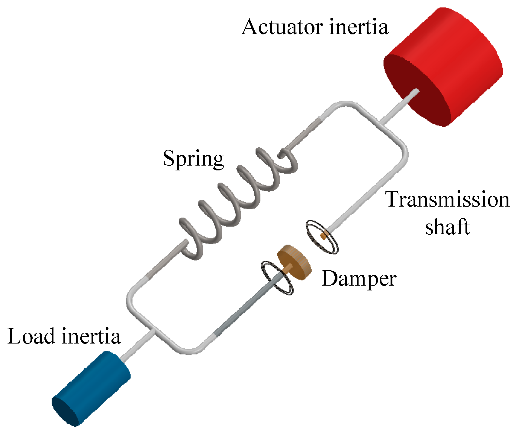
Figure 2.
Numerical simulation.

Disclaimer/Publisher’s Note: The statements, opinions and data contained in all publications are solely those of the individual author(s) and contributor(s) and not of MDPI and/or the editor(s). MDPI and/or the editor(s) disclaim responsibility for any injury to people or property resulting from any ideas, methods, instructions or products referred to in the content. |
© 2024 by the authors. Licensee MDPI, Basel, Switzerland. This article is an open access article distributed under the terms and conditions of the Creative Commons Attribution (CC BY) license (https://creativecommons.org/licenses/by/4.0/).
Share and Cite
MDPI and ACS Style
Hu, F.-R.; Hu, J.-S. On V-Geometric Ergodicity Markov Chains of the Two-Inertia Systems. Mathematics 2024, 12, 1492. https://doi.org/10.3390/math12101492
AMA Style
Hu F-R, Hu J-S. On V-Geometric Ergodicity Markov Chains of the Two-Inertia Systems. Mathematics. 2024; 12(10):1492. https://doi.org/10.3390/math12101492
Chicago/Turabian StyleHu, Feng-Rung, and Jia-Sheng Hu. 2024. "On V-Geometric Ergodicity Markov Chains of the Two-Inertia Systems" Mathematics 12, no. 10: 1492. https://doi.org/10.3390/math12101492
Note that from the first issue of 2016, this journal uses article numbers instead of page numbers. See further details here.