Abstract
The proliferation of Internet of Things (IoT) devices and their integration into critical infrastructure and business operations has rendered them susceptible to malware and cyber-attacks. Such malware presents a threat to the availability and reliability of IoT devices, and a failure to address it can have far-reaching impacts. Due to the limited resources of IoT devices, traditional rule-based detection systems are often ineffective against sophisticated attackers. This paper addressed these issues by designing a new framework that uses a machine learning (ML) algorithm for the detection of malware. Additionally, it also employed sequential detection architecture and evaluated eight malware datasets. The design framework is lightweight and effective in data processing and feature selection algorithms. Moreover, this work proposed a classification model that utilizes one support vector machine (SVM) algorithm and is individually tuned with three different optimization algorithms. The employed optimization algorithms are Nuclear Reactor Optimization (NRO), Artificial Rabbits Optimization (ARO), and Particle Swarm Optimization (PSO). These algorithms are used to explore a diverse search space and ensure robustness in optimizing the SVM for malware detection. After extensive simulations, our proposed framework achieved the desired accuracy among eleven existing ML algorithms and three proposed ensemblers (i.e., NRO_SVM, ARO_SVM, and PSO_SVM). Among all algorithms, NRO_SVM outperforms the others with an accuracy rate of 97.8%, an F1 score of 97%, and a recall of 99%, and has fewer false positives and false negatives. In addition, our model successfully identified and prevented malware-induced attacks with a high probability of recognizing new evolving threats.
Keywords:
intrusion detection; malware detection; Internet of Things; machine learning; optimization; classification MSC:
68-09
1. Introduction
In recent years, the surge in interconnected smart devices, known as the Internet of Things (IoT), has spanned industries like home appliances, vehicles, healthcare, and smart grids, offering convenience. However, widespread IoT adoption brings security challenges due to the lack of standardized security measures []. IoT devices, with lightweight protocols and low power consumption, become flexible but vulnerable to cyber threats, particularly malware. The absence of a comprehensive security protocol exposes devices to severe network attacks. The escalating accessibility of internet-connected devices intensifies cyber threats [], with new malware variants and development tools complicating accurate identification. Traditional security mechanisms, such as static or signature-based detection, struggle with zero-day attacks. In 2022–2023, the global count of IoT cyber-attacks surpassed 112 million incidents. This marks a substantial surge from approximately 32 million cases identified back in 2018 [].
Fixed-architecture machine learning algorithms are insufficient for detecting complex cyber breaches, necessitating advanced adaptive techniques for IoT security []. Traditional malware detection methods utilize both behavior-based and signature-based detection techniques. Signature-based detection involves comparing a program’s code against a repository of known signatures; if a match is found, the program is flagged as malware. While effective against established strains, it struggles with novel malware and requires frequent signature updates, demanding significant resources [,]. Behavior-based detection, on the other hand, focuses on monitoring program behavior rather than code, excelling in combating unknown or zero-day attacks. However, behavior-based detection may produce false positives and demands continuous system monitoring [].
To overcome these limitations, machine learning-based approaches are suggested. These involve training models on extensive datasets of known malware and benign programs, allowing the identification of new malware. Decision trees, support vector machines, and neural networks are common algorithms employed for malware detection []. Yet, these techniques face challenges, including the need for large and diverse malware datasets, susceptibility to bias, overfitting, and the “adversarial machine learning” problem, allowing attackers to manipulate input data [].
Deep learning algorithms seem to be a promising solution for malware detection and classification since deep learning algorithms can detect intricate patterns and features in data and quickly spot and react to novel, previously unnoticed malware. Nevertheless, deep learning models take a lot of computing power and time to train, which might be a problem for IoT devices [].
In the research community, machine learning-based techniques have made great strides in advancing the detection of malware in IoT devices. However, they have various limitations when applied to large datasets and struggle to find new and uncommon forms of malicious software. This is primarily due to the fact that the data in these datasets are highly dimensional and complex and cause scalability issues for an algorithm like SVM. Moreover, the SVM deployment of hyperparameters, such as the kernel type and the regularization parameter, is not flexible enough to capture the rapidly changing characteristics of novel malware strains. Furthermore, traditional SVM solutions to classification problems are unable to distinguish rarely encountered instances in the testing data due to class imbalance or a lack of representation in the training data. These shortcomings underscore the need for enhanced detection approaches to address the advancing danger of threats related to IoT. Some of the most effective methods to overcome these challenges are based on hybrid models that integrate various detection methodologies, thus enhancing and making the detection process efficient. The studies [,] recently unveiled the hybrid model, which integrates signature-based, behavior-based, and machine learning-based techniques to address the detection of known and unknown forms of malware. Through feature selection, the hybrid model integration improves efficiency by reducing dataset dimensionality, identifying proper attributes, and discarding irrelevant ones, which in turn reduces computational overhead [].
1.1. Understanding the Complexities of Securing IoT Devices
Recently, the rapid proliferation of IoT devices has led to various cybersecurity challenges caused by the interconnected nature of these devices. To form a well-rounded picture of the various challenges in securing IoT environments, it is important to discuss the shortcomings that render these devices vulnerable to cyber penetration.
- Resource limitation: IoT devices are normally considered resource-constrained. This inherently restricts the level at which adequate security can be implemented, making them vulnerable targets for actors with malicious intent.
- Outdated software and firmware: Despite the need to operate with the most current software and firmware, a vast number of IoT devices were unable to be updated due to a lack of updating mechanisms or existing ones being ineffective. As a result, a great many devices have widely recognized vulnerabilities that malefactors can take advantage of in order to compromise the security of the device.
- Weak authentication mechanism: Most IoT devices have an easily penetrable authentication mechanism that uses default or hardcoded passwords. In IoT, devices pose a low-bar authentication that permits malicious actors or cybercriminals to gain access to a device and network.
- Flawed encryption methods: The flaws in implementation and specific encryption technologies undermine the safety of the encryption process for IoT devices. This means that compromised encryption is likely to provoke a cyber-attack on the devices. Likewise, devices using that encryption will similarly be affected and may suffer data breaches for data extortion.
- Lack of standardization: There are a variety of devices that make up the IoT ecosystem, and they are developed and manufactured by various vendors. Often, each device has its own form of communication with other devices.
- Physical vulnerabilities: The presence of IoT devices in an uncontrolled environment raises the probability of physical exposure. An adversary with access to the hardware could take over the device or steal the data.
- Limited update capabilities: A substantial proportion of IoT devices cannot receive or install security updates on a regular basis. Therefore, they easily remain vulnerable to known threats.
By elucidating these specific deficiencies, we gain insights into the intricate challenges of securing IoT devices and can devise targeted strategies to bolster their resilience against cyber threats.
1.2. IoT Attack-Related Tangible Damage
The actual damage caused by the IoT is multifaceted and includes ramifications for operations, finances, and privacy. An example of a significant occurrence is a large-scale denial-of-service (DDoS) attack that was organized using hacked IoT devices []. The attacker normally creates a powerful botnet by taking advantage of flaws in networked devices, which disrupts a targeted internet service supplier and results in significant service unavailability. Organizations and enterprises incur substantial financial costs as a result of these attacks due to the disruptions in operations and the expenses associated with the analysis and resolution of cyber events [].
On the other hand, critical infrastructure can be disrupted as a result of attacks on the IoT environment. An attack on Industrial Internet of Things devices might lead to power outages, traffic congestion, etc. The affected sectors rely on these devices, from manufacturing to electrical networks []. Supply chains are affected by this operational disruption, which leads to inefficiencies and financial losses. IoT attacks may do serious harm in many ways, including violating people’s privacy. Unwanted monitoring and identity theft become more likely when security holes in household and healthcare IoT devices permit unauthorized access to private data [].
In addition, having the capability of modifying data adds an additional layer of risk. Modified readings from sensors or control signals in industrial IoT contexts might result in poor judgments, putting workers’ safety at risk and perhaps leading to mishaps or equipment damage. Critical sectors like hospitals and travel are also concerned about safety, as hacked IoT devices can endanger lives [].
One common topic in the wake of IoT hacks that affect companies as well as service providers is harm to reputation. When businesses neglect to safeguard their IoT infrastructure, confidence among consumers declines and there are implications for their brand perception. Regulatory agencies are increasingly holding businesses responsible for breaches of data and inadequate cybersecurity procedures, resulting in legal repercussions [].
The real-world consequences of IoT hacking attempts highlight the need for thorough cybersecurity plans, cooperative commercial initiatives, and regulations. Although IoT devices are interconnected, it is essential to actively minimize the different risks associated with their increasing ubiquity in everyday life.
1.3. Motivation and Contributions
Most existing studies on malware detection have focused on static or dynamic analysis, machine learning, or ensemble techniques, with some exploring hybrid analysis and big data approaches [,,,,]. AI-based malware detection is gaining attention, particularly through ensemble learning, which exhibits promise by training multiple classifiers. While signature-based detection is a prevalent approach, its effectiveness is constrained to identifying and mitigating just those malware versions that are already known. The integration of passive and active analytic techniques effectively tackles the challenge of deciphering concealed malware behavior; unfortunately, this comes at the cost of significant resource allocation []. The presence of a class imbalance between benign and malicious instances is a significant difficulty, requiring the implementation of strategies that address both balanced and unbalanced datasets [].
This study presents a novel optimized hybrid model for IoT malware detection, integrating support vector machines (SVM) with optimization methodologies. The design model improves the effectiveness of machine learning techniques by using mean decrease impurity (MDI) sequences of malware samples for feature extraction. Furthermore, it optimizes SVM parameterization, using NRO and ARO, to address overfitting concerns. Hence, the SVM will be optimized, and the identification efficiency will be advanced due to computational efficiency. Integrating static and dynamic analyses, SVM classification, NRO, ARO, and PSO optimization into a single ensemble learning methodology for continuous data streams on different devices has not been elaborated upon in the literature. Our optimized SVM models have substantially improved malware detection systems, and we provide practical insights into their key contributions.
- Enhanced SVM models: Three ensemble learning methods, NRO-SVM, ARO-SVM, and PSO-SVM, were developed to boost the performance of the traditional SVM method. These optimized SVM models leverage the full capacity of three distinct optimization algorithms, resulting in improved accuracy and efficiency in malware detection.
- Performance improvement: Our proposed algorithms outperform existing schemes by significantly reducing time complexity, mitigating overfitting, and efficiently handling large datasets while achieving an impressive accuracy range of 96% to 98%. This enhancement ensures the effectiveness of our approach in handling real-world data challenges.
- Adaptability and scalability: The proposed model demonstrates adaptability to newly discovered malware samples and effectively addresses the evolving nature of malware attacks. Moreover, its scalability enables it to handle large volumes of data without compromising accuracy or efficiency, making it suitable for widespread malware detection applications and contributing to the growing demands of cybersecurity.
The paper’s remaining sections are organized as follows: Section 2 briefly reviews related work in malware detection and classification. Section 3 elaborates on the proposed optimized hybrid model, including its components and operations. Section 4 presents the experimental outcomes and assesses the proposed model’s performance. Finally, Section 5 concludes the paper with a summary of our research.
2. Literature Review
A lot of research has been carried out in the field of IoT abnormality and intrusion detection to address issues and improve the accuracy of detection systems. Numerous strategies and algorithms have been used to provide outcomes that are solid and trustworthy.
The method set presented in [] is one noteworthy advancement in the field of anomaly detection; it uses recurrent neural network models to identify anomalies in Internet of Things settings. With respect to Dataset Kitsume, the system’s accuracy rating of 98% was achieved through the examination of sequential data patterns. But one important factor that has to be taken into account is the testing period, which was not specifically addressed in the study. This constraint makes it difficult to conduct a thorough assessment of its scalability and real-time suitability in extensive IoT setups.
A method for detecting and preventing attacks directed at IoT devices was presented by [] in the field of IoT attack detection. The method showed an impressive accuracy rate of 98.8% in accurately categorizing attack occurrences using the DS1-D1 and DS1-P datasets that contained examples of known attacks. Nevertheless, one of the most important shortcomings of this research is the use of an old dataset; recent attack trends and strategies are not included, affecting its application in real-world environments. To address the problem of secure analysis across a widespread IoT infrastructure, Taheri et al. [] proposed “federated approaches for multiparty computing using IoT devices”. Despite its accuracy rate of 56%, the algorithm was still unable to detect objects with a reasonable degree of accuracy, which warrants more exploration and enhancement. These solutions include testing with other deep learning architectures, expanding the set of training information sources, and tuning algorithm parameters.
To evade corrupted IoT devices, Wu et al. [] introduced the self-learning system D’IOT, reaching an accuracy rate of 95.6%. This constraint could be overcome by considering feature selection techniques, thus increasing not only detection accuracy but also overall efficiency. Future research could investigate more complex feature selection techniques, such as information gain or genetic algorithms. To spot IoT malware with an accuracy rate of 98%, Toldinas et al. [] added a DL-empowered LSTM method for malware based on opcodes. The study used a subpar dataset, and thus additional research with larger and more varied datasets is needed to determine the method’s utility.
Several authors have proposed DL-based methodologies to address IoT cybersecurity issues by enhancing detection and prevention mechanisms. Nisa et al. [] provided an accuracy of 99.20% using a DL-based technique to detect and prevent attacks by aggregating deep learning models. However, the model is not practical for real-world applications where the dataset does not include any IoT traffic or attack conditions due to dynamic and intricate patterns. Dhabal [] investigated RNN-based DL-powered intrusion detection with competitive recall and precision; however, its real-time application is restricted due to the model’s lengthy detection test period.
The academic industry has suggested a deep learning method for botnet identification that makes use of statistically determined network flow data that are acquired by using DNN []. The study’s astounding 99% accuracy rate attested to the efficacy of this strategy. Nevertheless, further investigation is required to completely evaluate the system’s performance in real-world scenarios, including testing duration computations. With 90% accuracy, Yilmaz et al. [] presented a deep learning-based algorithm to detect bots on online sites. The fact that detection accuracy may still be increased emphasizes how crucial it is to use feature selection strategies in order to increase precision. One of the study’s shortcomings was that it did not include a thorough analysis of relevant data, including testing time, confusion matrix, and other evaluative metrics.
The authors in [] recommended a deep learning approach for identifying botnets through the usage of DNN-obtained statistical network flow data. The model offers a 99% level of accuracy. However, more research will be necessary in order to fully assess the potential performance of this system in real-life circumstances, such as computations of testing time. Yilmaz et al. [] suggested a deep learning-based algorithm to identify bots on the internet but with a lower accuracy of 90%. Hence, there is a need to adopt feature selection techniques, given that detection levels can still be optimized.
The authors in [] presented a bidirectional long short-term memory (BLSTM) that achieved an accuracy of 99% in packet-level detection in IoT. However, the authors failed to provide sufficient details on the testing time, in-depth ROC curve, and confusion matrix. Another study used Q-learning to identify malware on mobile devices, and it achieved 67% accuracy []. Although 99.14% accuracy was claimed for enhanced intrusion detection utilizing deep belief networks and probabilistic neural networks, important parameters like false positive and false negative rates were absent. Notwithstanding the progress made [], further investigation is required to surmount constraints and augment precision, efficacy, and relevance in actual Internet of Things contexts. Table 1 shows a compressive summary of the above-discussed literature.

Table 1.
Overview of the literature.
In view of the current literature and research progress in this area, there is still a need for robust algorithms for malware detection, given the significant increase in attacks, as indicated by Figure 1.
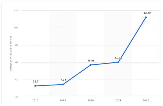
Figure 1.
Prevalence of IoT cyber-attacks.
Despite the progress that has been made, additional research is required to overcome constraints and improve accuracy, efficiency, and applicability in Internet of Things contexts. Our proposed optimized malware detection framework is detailed in Section 3.
3. Materials and Methods
This article employs a hybrid approach, utilizing 8 malware datasets (see Section 3.1) to develop a machine learning model for malware detection. First, the dataset is loaded into data frames, and then all of the datasets that include the target column are merged together, with the target column being classified as either malicious or benign. Subsequently, exploration data analysis (EDA) uncovers data patterns. To address the imbalance, the target variable distribution is adjusted to prevent overfitting. Feature engineering techniques, including one-hot encoding, are applied for data transformation, while feature scaling standardizes data within the range of independent variables.
The XGBoost algorithm and mean decrease impurity (MDI) identify the most crucial features integrated into the Zeek Analysis Tool (ZAT) data frame for the efficient handling of large datasets. With the help of the silhouette score measure, the studied data are clustered using the k-means and principal component analysis techniques. Then the data are prepared for machine learning analysis using the method of an isolation forest, which detects abnormalities and outliers in the data. The data are separated into 25% for testing and 75% for training. The SVM parameters are optimized based on the NRO, ARO, and PSO methods.
Furthermore, 11 out of the best techniques are used for validation of the model, including normalized cross-correlation (NCC), decision tree classifier (DTC), logistic regression (LR), SVM-GridSearch, Naïve Bayes (NB), XGBoost, linear model (LM), UnTuned-SVM (UTSVM), ADAboost (ADA), linear discriminant analysis (LDA) and k-nearest neighbor (KNN). Performance metrics include accuracy, Matthew’s correlation coefficient, precision, confusion matrix, recall, ROC, complexity, and F1 score to evaluate the performance of proposed and previous state-of-the-art models. Figure 2 illustrates the suggested model’s flow chart, with detailed steps discussed in the subsequent subsections.
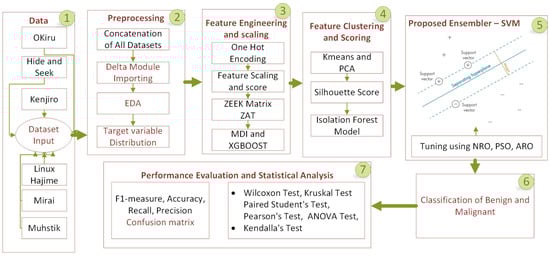
Figure 2.
Comprehensive flow diagram for the hybrid system model.
3.1. Dataset
The IoT-23 dataset comprises current network traffic data from diverse IoT devices, featuring eight instances of adverse activities involving various malware-infected devices. Additionally, three benign scenarios represent regular IoT device traffic []. These scenarios are embedded in eight network captures (PCAP files) from infected IoT devices and three captures displaying network activity from legitimate IoT devices. PCAP files rotate every 24 h to accommodate prolonged malware execution, though certain files may terminate prematurely due to rapid growth, leading to varied capture times. Table 2 details the eight malicious scenarios, providing information on ID, dataset name, operation hours, packet count, and Zeek ID flows from the conn.log file. The table also includes details on the size of the original PCAP files and potentially the identity of the malware sample infecting the device. Recognized as a vital resource, the IoT-23 dataset supports IoT security exploration, aiding algorithm enhancement and serving as a valuable tool for training and evaluating IoT security solutions.
Table 2.
Malicious IoT devices (summary) [].
3.2. Preprocessing
Before we applied classification methods to our data, we employed various techniques for analyzing and pre-processing it. First, we loaded all the data into a single data frame and concatenated it with the target column.
The pre-processing steps were thereafter executed in a sequential manner, and we will now elaborate on each step in a comprehensive manner.
3.2.1. Target Variable Distribution
The target variable in malware detection often takes on a binary form, designating whether a particular sample is dangerous (coded as 1) or benign (coded as 0). The distribution pattern of the target variable is of utmost significance because it has a substantial influence on the efficiency with which the ML model is being utilized for detection functions []. If there is a considerable imbalance in the distribution of the target variable, characterized by a large number of benign occurrences and a small number of malicious cases (or vice versa), the model may become biased and favor the majority class. In an illustrative scenario where the distribution of samples consists of 95% benign samples and 5% malicious samples, a basic model that consistently predicts the benign state would yield an observed accuracy of 95%. But by its very nature, this model would be unable to recognize any of the potentially malicious samples. Different statistical measures are used as quantifiers in order to evaluate the target variable’s distribution. Among these metrics are the proportion that contains harmful instances, the total number of data points in each class, and the mean and variance of the intended parameter. Equation (1) can be used to definitively state this:
where n_mal means the number of malicious samples and n_ben means the number of benign samples. Considering p as the proportion of detrimental samples, with nmalicious denoting the count of malicious samples, and nbenign indicating the count of benign samples, an alternative approach to calculate the mean as well as the variance of the target variable has been outlined [], presented in Equations (2) and (3):
Both the variance and the mean of the target parameter are important statistical measures in the field of malware identification. The mean or average value of the target variable provides a close representation of the proportion of malicious samples present in the collection.
Within the extensive domain of statistical analysis, the concept of variance unveils its complex characteristics, demonstrating the degree to which the target variable deviates from the alleged mean value. These significant metrics provide us with access to a vast amount of information, offering invaluable perspectives on the intricate nature of the distribution of the target variable. As we set off on our quest in the vast ocean of machine learning models to determine which one is the most accurate in detecting malware, the statistics outlined below are nothing short of critical to evaluate the efficiency and abilities of our models with rigorous scrutiny.
3.2.2. One-Hot Encoding for Feature Engineering
Each malware sample from the provided dataset is defined specifically for malware classification. An 8-bit vector and the method of one-hot encoder are used to realistically present different types of viruses. Specifically, the method defines that every point in the vector is a unique type of virus []. To illustrate, the Gagfyt malware type could manifest as [1, 0, 0, 0, 0, 0, 0], while the Hide and Seek malware type could be denoted as [0, 1, 0, 0, 0, 0, 0, 0]. The result is a single hot encoded vector engaging that uniquely identifies the relevant malware class, hence trimming down the effort of representing each and every element in our entire collection. To illustrate, the order [0, 0, 0, 0, 1, 0, 0] gets used to represent a specimen that has been tagged as Muhstik. The same process is used consistently for all of the samples in our dataset.
Malware labels are transformed into vectors using a single-hot encoding process. Moreover, machine learning algorithms built expressly to identify as well as classify malware use these vectors as inputs. Through the analysis of these vectors, the algorithms are able to identify complex relationships and patterns between various malware strains by analyzing their unique one-hot encoded representations. The algorithms are then enabled to classify fresh malware samples in accordance with their different kinds by means of the information that has been obtained.
3.2.3. Feature Scaling
Samples tagged with different kinds of malware, such as Gagfyt and Hide and Seek, are included in the malware data collection. These samples may have different ranges, which makes assessment and comparison more difficult. Feature scaling, a critical preprocessing step, standardizes the range of these features, enhancing the effectiveness of machine learning algorithms [].
To achieve uniformity among feature values, we adopt normalization, gracefully rescaling them to a range between 0 and 1. The process involves uncovering minimum and maximum feature values across all malware samples. Equation (4) is given by []:
Consider the malware specimen Gagfyt, with properties measuring 100, and mirai, measuring 50. Applying normalization to these values involves utilizing the unique minimum and maximum values for each feature within the dataset. For Gagfyt, with values ranging from 50 to 500, and mirai, with values ranging from 20 to 200, the normalization equation unveils a symphony of scaled magnitudes.
Normalized Gagfyt value: , The result is 0.1876. This indicates that the average value of the Gagfyt attribute for this sample is 0.1876, as stated.
Normalized mirai value: , the output is 0.326. This indicates that the normalized mirai feature value for this sample is 0.326.
The transformative power of attribute scaling ensures harmonious proportions among features, facilitating precise comparison and analysis. By placing all feature values on the same scale, machine learning algorithms, when applied to our dataset, exhibit enhanced performance and accuracy of malware categorization.
Practical issues become critical in circumstances where the endless nature of the incoming information makes its range unpredictable. Statistical metrics created from the given data are a regularly used method in handling such cases. For the aim of data standardization, we employ reliable statistical metrics like the mean and standard deviation over global minimums and maximums. For the purpose of standardizing the data and converting them to a conventional normal distribution, the mean is subtracted, and the deviation from the mean is divided. This technique has proven to be reliable and broadly applicable, especially when the input data range cannot be explicitly defined. Our scaling procedure guarantees flexibility to the intrinsic characteristics of the data by utilizing statistical measures that are directly extracted from the dataset. This technique improves the flexibility and reliability of our analysis in situations where the exact spectrum of input data is uncertain.
3.2.4. Feature Importance
Feature importance is integral for understanding machine learning model predictions, especially in malware detection, aiding in recognizing and classifying essential malware traits. XGBoost is the most popular algorithm for accurate malware models which relies on the MDI technique to determine the importance of features. This approach measures how much impurity is diminished when splitting the data with respect to a given feature, hence identifying important features for detecting malware.
Moreover, one must have access to the feature significance property to obtain and rank the scores, and the model must be fit to determine the importance of the attributes in XGBoost for the identification of malware using MDI. Thereafter, the scores are studied to identify the distinct characteristics that malware have in common, which can be the basis for improving the acquired model. Moreover, this discovery improves efficiency due to the reduction in the same components, simplicity, and better performance but also detection accuracy. The method is effective in detecting and categorizing malware as it emphasizes the major infection signs [].
3.2.5. Zero Access Tool (ZAT) to Convert Dataframe to Matrix
ZAT is a standalone Python program that can process multiple file formats, but it was designed to analyze and visualize malware data exclusively. The functionality DataFrame to Matrix offers an opportunity to generate a matrix representation from the malware-related data that are stored in a data frame, as it is infeasible to use matrices directly. In order to scale numerical features and encode categorical data, one must transform the matrix, making it possible to apply machine learning recommendations to instances, such as clustering and classification [].
Mathematically, the transformation of a data frame to a matrix representation can be formulated in the following way: the original DataFrame X introduced in Equation (5) is presented with n rows and m columns, while a row is a sample, and a column is an attribute:
Let denote the i-th feature in the feature set . Let be a matrix depiction of the target variable , where each row corresponds to a sample, and every column represents a feature. This is in accordance with Equation (6) [].
The term “hi(yk)” in the given scenario denotes the numerical value assigned to the i-th feature for the j-th sample. Depending on the properties within the original data frame, various encoding and scaling techniques may be applied before transforming the data into a matrix representation.
3.2.6. Making Clusters Using k-Means and PCA
k-means and PCA clustering are valuable techniques for malware detection because they help to collect malware samples that have identical characteristics. It may be simpler to find various malware and more accurate to detect the various changes happening in the data under testing.
PCA and k-means clustering were used in [] to identify malware cases. The dataset should undergo feature engineering and preparation to identify distinguishing features for different malware instances. PCA is used to find a reduced set of orthogonal axes that encapsulate the most important variance in data. In this way, the dimension of space in which the feature space exists is fundamentally reduced. Later on, k-means clustering is applied to group malware samples in this lower-dimensional feature space according to their newly generated feature representation. The primary objective of k-means clustering is to partition a dataset X with n malware samples (C1, C2,…, Ck), each characterized by m attributes, into k different clusters. In order to facilitate clustering, Equation (7) reduces the overall linear length [] among instances of malware Xj and their center points µi.
When PCA is implemented, the aim is to transform dataset X, comprising n malware samples, each with m features, into a new set with k features. This transformation is designed to maximize the extraction of variance from the data. ‘Ci’ in this method denotes the collection of instances of malware that are associated with the node of the cluster i’s centroid. The transformation is governed by Equation (8), as outlined below.
where X’s covariance matrix’s k orthogonal eigenvectors and W’s matrix have the same k greatest eigenvalues.
After categorizing the malware samples with k-means clustering and PCA, it becomes possible to identify various types of malwares. These types include Gagfyt, Hide and Seek, Kenjiro, Linux Hajime, Mirai, Mu-hstik, Okiru, and Tori, which are useful in the classification of malware.
3.2.7. Silhouette Score
Silhouette scoring assesses clustering quality by evaluating how well clusters group instances. A high score indicates effective clustering, which is crucial in malware detection. This tool helps identify shared traits in malware samples, aiding the detection of new strains. In malware detection, silhouette scoring evaluates clustering algorithms depending on patterns like mirai and okiru. Let X be the feature vectors representing malware. A clustering method then yields C clusters, and the cluster of instances I is denoted by c(i). Equation (9) uses trait-based clustering to efficiently identify emerging risks by calculating the silhouette coefficient for each occurrence I in X [].
The silhouette scoring tool assesses cluster quality by evaluating the effectiveness of clustering instances within clusters and cluster divisions. Where a high score indicates successful clustering, the measure aids in uncovering novel malware strains and uncovering inherent qualities. The effectiveness of a clustering algorithm based on its ability to identify malware is ascertained by computing each element’s silhouette coefficient in dataset X. The coefficient ranges from −1 to 1, and a value of 1 indicates an instance that is best attuned to remaining in its cluster. The distance is calculated as the average silhouette coefficient, according to Equation (10), which measures dissimilarities between instances in other clusters and within the same cluster [].
where |X| is the number of instances in set X.
Equation (10) shows how we can consider the efficiency of our clustering algorithm in accurately putting similar malware samples into one group. A high silhouette score will indicate how quickly we can differentiate clusters and the presence of similar instances in a cluster. Then, our clustering algorithm efficiently reveals distinct patterns in these malware samples.
3.2.8. Model of Isolation Forests
The use of the isolation forest technique for malware detection [] illustrates a novel machine learning approach that can aid in unraveling the mechanics of malevolent malware. This method seeks to identify heterotypic patterns, including virus samples, by forming random decision trees that distinguish them from the majority of instances. The random forest of the model, trained and tested with the aforementioned features X for normal malware datasets, then isolates previously undetected malware with heterozygous behavior patterns. By utilizing the dividing criteria and replication functions, the isolation forest locally isolates the data points. The abnormality of a given data point is represented by a single, h(x), which measures the number of times that the particular data point has actually been isolated by selecting hyperplanes. The lower the h(x), the higher the anomaly, as exemplified by malware samples with heterozygous feature assortment [].
The model further considers several parameters, including the normalization factor, C(n), the aggregate number of data points, and the average route length a data point x takes across all trees, E(h(x)). Higher values of the anomaly score, s(x), indicate more substantial irregularity. The score ranges from 0 to 1. The program, which was trained on existing malware samples, recognizes new and possibly hazardous samples that display unique behavior. It then marks such samples as anomalous and proposes a new malware.
3.3. Model of Ensemble Classification
Support vector machines (SVM) are used as the main classifier in this study, along with optimization techniques. The ensemble approach has also been validated using eleven state-of-the-art methods. A thorough explanation and assessment of each model are provided below.
3.3.1. SVM
A potent supervised learning tool for classification, regression analysis, and anomaly detection is the support vector machine (SVM) []. SVMs look for the best hyperplane to divide data into different groups. The margin is determined by how far the hyperplane is from the closest points (also known as the support vectors) in each class.
Depending on the kernel function selected, an SVM’s decision boundary may be linear or nonlinear. The input data are transformed by the kernel function into a higher-dimensional feature space, enabling nonlinear data separation. The linear, polynomial, radial basis function (RBF), and sigmoid kernel functions are often utilized. The SVM optimization problem can be expressed mathematically as follows [] in Equation (12):
and are the input feature vector and label for the training example, where b is the bias term and w is the weight vector. C is a hyperparameter that manages the trade-off between increasing the width of the margin and decreasing the classification error, and I is the space variable that permits soft margin classification.
Typically, quadratic programming approaches tackle optimization, which entails minimizing a quadratic objective function while adhering to linear constraints. The best solution to the Lagrange dual issue may also be determined, leading to the construction of the SVM as a linear combination of support vectors [], as in Equation (13):
The Lagrange multiplier is I, the bias term is bs, and the kernel function is K(zu, z). The non-zero Lagrange multipliers of the support vectors determine the decision boundary’s placement. The optimized version of SVM is graphically presented in Figure 3.
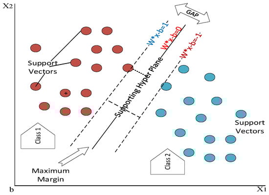
Figure 3.
Optimized SVM representation.
3.3.2. Artificial Rabbits Optimization
ARO is a metaheuristic optimization method inspired by rabbit foraging behavior []. In the domain of malware classification, ARO is utilized to discover the optimal hyperparameters for support vector machines (SVMs). SVMs are widely employed in malware classification tasks due to their effectiveness in handling large datasets and non-linearly separable classes. The selection of appropriate hyperparameters, such as the bias term, normalization parameter, and kernel function, significantly influences the performance of SVMs. The ARO algorithm working flow is shown in Figure 4. The arrows shows the data flow in the process.
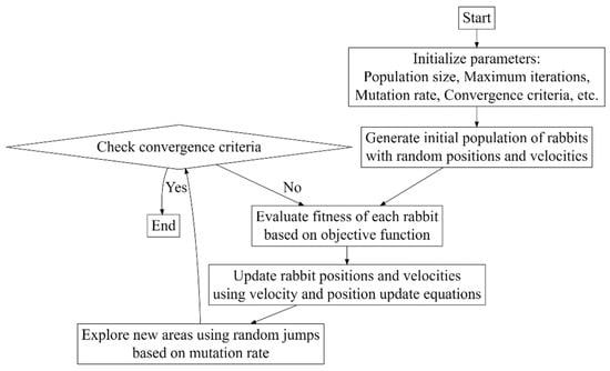
Figure 4.
ARO steps for finding the optimum solution.
In the application of ARO to SVM hyperparameter optimization, the solution domain is explored using a population of artificial rabbits. These rabbits are categorized into three groups based on their behavior: explorers, exploiters, and breeders.
- Explorers are moving across the solution space randomly, visiting different regions. They help to implement the exploration part of the optimization when all areas of the solution space are reviewed.
- Exploiters are more concentrated and move closer to the best solution that has been found so far. In this process, they exploit certain information retrieved through the exploration part to refine the solutions. Therefore, exploiters implement exploitation.
- Breeders generate new solutions by combining the concepts exploited by exploiters. This obviously helps to maintain population diversity by combining attractive solutions.
The ARO algorithm employs three unique artificial rabbit behaviors, namely exploring, exploiting, and breeding, to dynamically adjust the behavior of artificial rabbits. ARO uses breeds to ensure that a bunny continues to explore more regions of the arrangement space, exploring both variations and promising regions to refine solutions. Because ARO balances both approaches, using ARO to discover optimal or near-optimal configurations for SVMs in malware classification is effective.
In SVM-based malware classification, the fitness function is measured with model accuracy as well as complexity. ARO optimizes the hyperparameters of SVM, including the kernel function, kernel parameters, regularization parameter, and bias parameter to improve performance. The decision boundary is tuned to optimally separate malware and non-malware classes, as defined in Equation (14) []:
This technique optimizes hyperparameters in SVM for malware classification. It explores the hyperparameter space to select the optimal kernel function and parameters, balancing the accuracy and the model’s complexity. The kernel, therefore, is chosen in such a way that data are most effectively transformed for linear separation. Accuracy is measured using validation or cross-validation, and complexity is controlled using support vectors or the regularization parameter [].
3.3.3. Nuclear Reactor Optimization (NRO)
Model name = Nuclear Reactor Optimization, short name = NRO. NRO maintains the tradeoff between exploration and exploitation by a dynamic process inspired by nuclear reactors. NRO uses the principle of the process in a nuclear reactor to optimize hyperparameters in malware detection with a major focus on SVM []. The process in a nuclear reactor is based on the two principles of fission and neutron absorption:
- Fission refers to the splitting of nuclei to create new candidate solutions that could be explored. In the context of optimization, fission refers to the exploration nature of the problem as new solutions are created by expanding the search space.
- Neutron absorption also improves the current solutions via the absorption of neutrons. This is the exploitation part of the optimization process, which involves improving the solutions found by using the information acquired from the exploration part.
In the optimization process, NRO tunes hyperparameters such as the kernel function, regularization, and bias term for SVMs used in malware detection. It achieves this by randomly dividing solutions, updating them with random values inspired by the fission and neutron absorption principles, and evaluating their fitness based on SVM correctness. The steps are shown in Figure 5.
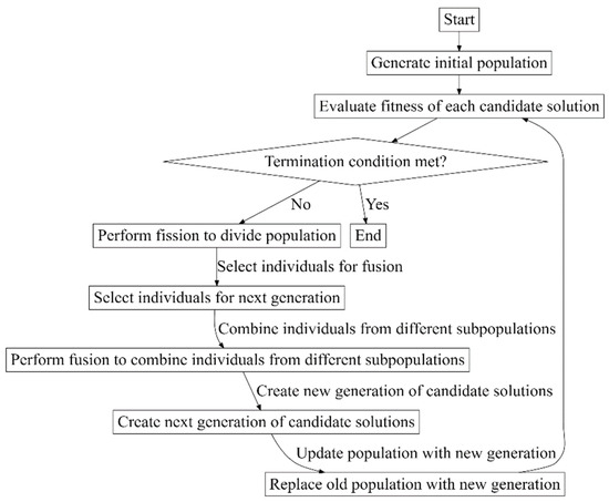
Figure 5.
NRO steps for finding the optimum solution.
By dynamically balancing the generation of new solutions through fission and the refinement of existing solutions through neutron absorption, NRO effectively maintains the exploration and exploitation tradeoff. This ensures that the optimization process explores diverse regions of the solution space while also exploiting promising areas to improve the quality of solutions, ultimately leading to the discovery of optimal or near-optimal hyperparameter configurations for SVM-based malware detection.
The fitness function and parameter optimization are expressed in Equations (15) and 16, showcasing NRO’s role in refining SVM for enhanced malware classification.
The ARO approach is used to search the hyperparameter space for the ideal kernel function and its parameters that optimize the accuracy of the SVM model while minimizing its complexity. Accuracy may be assessed using a validation set or a cross-validation approach. The number of support vectors or the value of the regularization parameter can be used to determine the complexity.
3.3.4. Particle Swarm Optimization (PSO)
PSO is a metaheuristic algorithm that models a swarm of particles moving in a search space to find the optimal solution []. Each particle in the swarm represents a candidate solution. In malware detection, PSO can tune the hyperparameters of an SVM. The optimization process involves the following steps:
- Create a swarm of N particles with positions and velocities , where and and are n-dimensional vectors.
- Evaluate the objective function for each particle’s current position .
- Initialize the personal best position and the global best position .
- For each iteration :
- Update the velocity of each particle using the velocity update equation:
- where w is the inertia weight, c1 and c2 are the acceleration coefficients, and rand() is a random number between 0 and 1.
- Update the position of each particle using the position update equation:
- Evaluate the objective function for each particle’s new position .
- Update the personal best position if is greater than .
- Update the global best position if is greater than .
- Return the global best position as the optimal solution.
Each particle’s location in this situation denotes a set of SVM hyperparameters. The PSO algorithm iteratively adjusts these hyperparameters to maximize the classification accuracy of the SVM. The objective function indicates the SVM’s classification accuracy using those hyperparameters. The PSO approach explores the hyperparameter space for the set that optimizes the SVM’s classification accuracy on a given dataset. Graphically the steps for finding an optimum solution are shown in Figure 6.
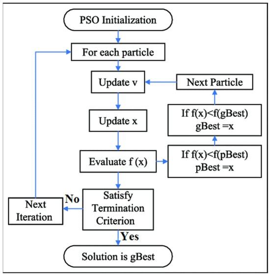
Figure 6.
PSO steps for finding the optimum solution [].
The exploration and exploitation tradeoff is maintained through the collective behavior of particles navigating the search space.
Exploration: In PSO, exploration is facilitated by the stochastic movement of particles through the search space. Each particle represents a potential solution, and its position in the search space corresponds to a candidate solution. During the exploration phase, particles explore the search space by adjusting their positions based on two key factors:
- Global best position: Each particle is aware of the best solution found by any particle in the swarm. This global best position serves as a guide for exploration, pulling particles toward promising regions of the search space.
- Local best position: Each particle keeps track of the best position it has ever encountered when moving. The local best position influences the particle to search the surrounding area of the search space.
The stochastic movement and interactions with both global and local best positions allow particles to search various parts of the search space, which leads to searching for new solutions.
Exploitation: The exploitation in PSO includes promising solutions or findings, refining and modifying the search process. Particles modify their velocities as they traverse the search space to get closer to the optimal solutions or suboptimal regions. The velocity updating equation in PSO is based on two main parts:
- The cognitive component directs a particle towards its personal best position, thus promoting the exploitation of the local solution.
- The social component directs a particle towards the global best found by a particle, thus exploiting the entire swarm.
The exploration and exploitation are balanced through particles’ interaction with global and local best positions while managing the velocities by continuously adjusting according to personal and global best positions. The exploration is based on the initial position, while exploitation is through the possible situation they have identified. Thus, in the above expression of PSO, the search mechanism proceeds through the exploration of different parts of the search space while exploitation refines the exploration process through convergence to an optimal point.
4. Experimental Results
The proposed model is implemented with TensorFlow on the Google Colab environment using the premium GPU-based end-to-end open-source ML platform.
The experimental process consists of recording the feature obtained from incoming packet data extracted from a prespecified set of features given by the category. To simplify processing complexity, a feature selection approach will be adopted. Corresponding features are extracted from the input traffic pattern as a pre-processing step. Subsequently, the packet data extracted are sequentially passed through individual attack detection sub-engines. Figure 7 illustrates boxplots showcasing the distributions of various features within the dataset. Each boxplot offers a visual representation of a specific feature’s distribution, with the median represented by the central line, the interquartile range (IQR) depicted by the box, and the whiskers extending to illustrate the data range. Any outliers, if present, are also depicted as individual points lying beyond the whiskers. This graphical representation facilitates the examination of the spread and variability of each feature, aiding in the detection of potential outliers and enhancing comprehension of the dataset’s overall distribution characteristics.
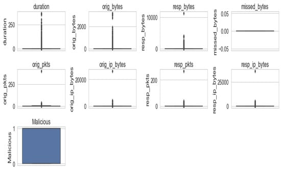
Figure 7.
Exploring the distribution.
The core component of this proposed framework is the attack detection sub-engines responsible for identifying various types of attacks. Multiple sub-engines comprise the detection engine, each dedicated to detecting specific attack types. The number of distinct sub-engines depends on the number of attacks in the training database. In our proposed framework, firstly, the entire dataset is loaded into data frames. Then, the Traffic column is labeled with the malicious type, and if it is benign, the values are simply kept as benign. Furthermore, unnecessary columns are dropped during the pre-processing stage, and white spaces are removed before and after the string. The next step involves filtering out portscan packets, okiru packets, and other malicious packets, such as DDOS and C&C.
Next, we apply target variable distribution to some columns to observe malicious and benign data distribution, as depicted in Figure 8.
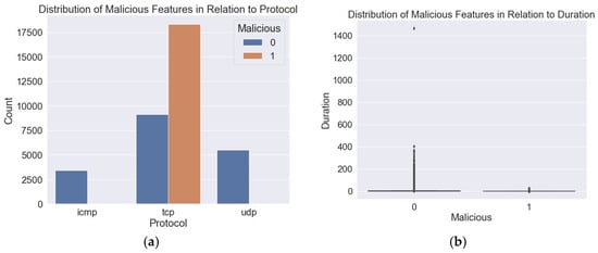
Figure 8.
Exploring the distribution of malicious features in relation to other dependent variables. (a) Feature protocol distribution; (b) Feature duration.
Figure 9 illustrates our further exploration of the data to analyze the outliers present in the data. The correlation of data indicates that the records in the dataset are more relevant. However, some records significantly differ from the actual data and are considered outliers.
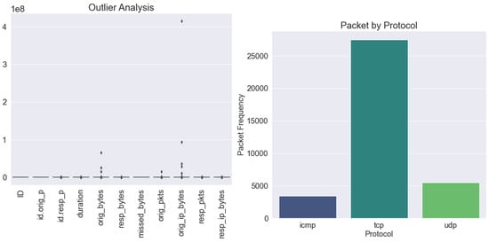
Figure 9.
Outlier analysis and packet counting w.r.t different protocols.
Moreover, when examining the quantity of packets received from various protocols, it is evident that there is a greater number of packets for TCP in comparison to UDP and ICMP. This discovery highlights the need for greater scrutiny prior to categorization. Furthermore, we created a customized diverging color map pattern to represent the features and showcased their significance using a heatmap, as depicted in Figure 10. It also illustrates the correlations between the dataset’s numerical characteristics. The intensity and direction of correlations are clearly communicated by the color gradient that moves from warm to cold tones. Strong positive associations are shown by abundant red hues, while strong negative correlations are indicated by deep blue hues. Near zero, lighter hues indicate minuscule or moderate associations. The identification of feature interdependencies and the strategic choice of characteristics for modeling are greatly aided by this depiction. It also helps identify multicollinearity issues, offering a concise yet informative assessment for intelligent decisions in further investigations and modeling projects.
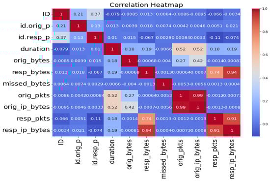
Figure 10.
Heat map correlation analysis of features and their dependency.
The MDI method, often employed alongside XGBoost, is a widely recognized technique for feature selection. It assesses the importance of each feature by examining how much it contributes to reducing impurity when included in the decision tree. In essence, it measures a feature’s impact on the decision-making process of the tree. The results of the MDI analysis, as depicted in Figure 11, show the relative significance of each feature in the dataset, with importance typically expressed as a percentage. Features are ranked based on their importance, with those contributing most significantly assigned higher percentages. Understanding Figure 11 requires recognizing that features with higher importance scores are more influential in shaping the model’s output. Therefore, prioritizing features with high-importance scores is advisable, as they offer valuable insights into explaining the target variable. When many features exhibit comparable relevancy assessments, further investigation utilizing methods like correlation analysis or feature selection algorithms might assist in determining the most vital group of information for the predictive algorithm.
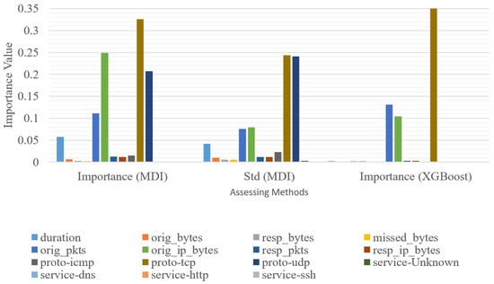
Figure 11.
Evaluating the significance of features in target prediction analysis.
We employed the ZAT data processing module to manage categorical data, ensuring explicit conversion before inputting them into the transformer. The analysis and grouping of malware samples involved the application of two widely recognized techniques, namely k-means and PCA clustering. The findings are presented in Figure 12, which illustrates the visualization of grouped data points in two or three dimensions following PCA reduction and k-means clustering. The resulting plot visually shows each individual data point as a colored dot, serving as an indicator of its respective cluster. Figure 12 aids in identifying patterns or trends, offering insights into malware behavior and characteristics. Clusters are distinctly separated, suggesting notable dissimilarities within each cluster. Silhouette scoring assessed clustering quality by calculating the average distance within a cluster and spacing to the nearest neighboring cluster.
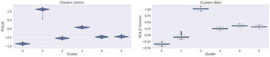
Figure 12.
Clustering for different group identification based on silhouette scores.
Higher values of silhouette scores, a scale from −1 to 1, suggest better clustering outcomes. If a data point has a score of 1, it is successfully assigned to its designated cluster and not to any neighboring clusters. Conversely, a score of −1 indicates that the data point is given to neighboring clusters rather than its own cluster.
The next step involves forwarding the data to classification methods. We began by tuning the hyperparameters of the ARO_SVM, NRO_SVM, and PSO_SVM. The hyperparameters are passed through the optimization methods, and then the model is trained and evaluated on each combination of the SVM. Optimization methods help find the best solution for handling large malware data. The best combination of parameters determined by different optimization methods is presented in Table 3.
Table 3.
Optimized parameter values by metaheuristic algorithms.
In order to evaluate our model, we conducted an assessment of the performance of the ARO_SVM, NRO_SVM, and PSO_SVM algorithms. This evaluation involved optimizing the hyperparameters of the SVM model through these aforementioned optimization methods. The optimization techniques successfully acquired the optimal parameters for SVM, as outlined in Table 3. These parameters were subsequently employed in the training and testing processes. Furthermore, we assessed the performance of the proposed model by calculating the true positive and true negative values, which are graphically shown in Figure 13a for both the proposed and existing techniques. Figure 13b shows how three proposed optimized algorithms (ARO_SVM, NRO_SVM, and PSO_SVM) work to find the best kernel function for detecting malware. The x-axis tracks the number of iterations, or rounds of optimization, while the y-axis measures the loss incurred during each iteration. It can be interpreted that the lower the values on the y-axis, the better the optimization.
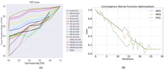
Figure 13.
ROC curve analysis and optimization algorithm convergence. (a) ROC Curve Analysis; (b) Convergence of Optimization Algorithms.
Firstly, we can observe the algorithms’ behavior with time. ARO_SVM and NRO_SVM both have a gradual decrease which proves that they are constantly improving. Meanwhile, PSO_SVM has many ups and downs, showing that sometimes it does not find the optimal solution. Thus, analyzing the plot above, one can learn which of the algorithms minimizes loss better, and hence gives the resulting optimal kernel function that is used for detecting malware.
ARO_SVM, NRO_SVM, and PSO_SVM have great results in efficiently managing large datasets and achieving good accuracy scores and ROC curve values. The SVM model has been tested for accuracy values. The accuracy values are shown in Figure 14 below. The range of accuracy values falls between 0 and 1. If the value is closer to 1, the accuracy score is high; otherwise, the score is low if it is closer to 0.
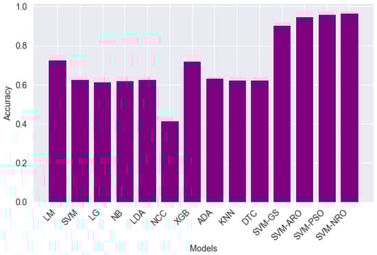
Figure 14.
Performance evaluation of accuracy values.
As shown in Table 4 below, performance metrics of various algorithms were evaluated using five-fold cross-validation for the considered dataset. Specifically, each fold was a split of the data, with one fold used as the test set and the remaining used for training. In different folds, the corresponding F1 score, accuracy, precision, and recall metrics for each algorithm are displayed in the table below. This means that for each fold, F1 score, accuracy, precision, and recall were obtained and analyzed for all algorithms. Furthermore, at the end of the table, average values of these performance measures across all folds are presented. Among all algorithms, the performance of NRO_SVM is remarkable and the highest.
Table 4.
Accuracy values of the proposed scheme and existing methods.
For the purpose of determining the accuracy of binary classification, Figure 15 utilized the Matthews correlation coefficient (MCC), considering true positives, true negatives, false positives, and false negatives. This indicates that the model is performing better in terms of successfully identifying malware samples when the MCC value is higher. An MCC value near 1 indicates accurate predictions, while values closer to 0 or −1 suggest incorrect predictions. NRO_SVM achieves a 93% MCC value and outperforms other existing and proposed optimized methods. The statistical analysis in Table 5 validates the hypothesis acceptance rate for existing and proposed methods.
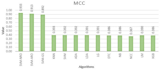
Figure 15.
MCC values of existing algorithms and proposed ensemble methods.
Table 5.
Statistical analysis of the models.
The system under consideration consists of two main components: a feature selection module and a model selector module. The feature selection module is responsible for reducing the number of original features, while the model selector module is designed to identify classifiers that demonstrate superior performance in terms of accuracy and processing times for each sub-engine. Our “hybrid” categorization approach produces a lighter and more accurate system than the traditional detection architecture.
Table 6 intends to give an in-depth understanding of the technical advantages and disadvantages of each model. Researchers, practitioners, and cybersecurity specialists who want to understand the intricacies of cutting-edge malware detection techniques may find it very helpful. The features that have been emphasized provide a thorough understanding of the models’ capabilities and aid in decision-making when choosing an appropriate strategy for IoT malware detection.
Table 6.
Comparison of the technical aspects with the recent trend.
5. Conclusions
This study aimed to design a detection framework to counter the escalating cyber-attacks targeting IoT devices. By employing advanced techniques in feature selection, distribution, and clustering, our primary objective was to achieve precise and efficient detection capabilities. Our proposed detection framework, integrating hybrid classification methods such as ARO_SVM, NRO_SVM, and PSO_SVM, exhibited remarkable proficiency in identifying diverse types of attacks on IoT devices, including both known and novel threats. Notably, NRO_SVM emerged as the most accurate method, boasting an impressive F1 score of 0.962 and an accuracy of 0.978. The implications of our findings are substantial for the cybersecurity domain, particularly within IoT ecosystems. The ability to accurately detect and mitigate cyber threats can significantly enhance the security posture of IoT environments. Moreover, the lightweight nature of our framework ensures minimal resource utilization, making it suitable for deployment in resource-constrained environments.
Future research endeavors will focus on several areas for improvement. Extensive validation of our detection framework in diverse IoT environments will be undertaken to evaluate its performance under real-world conditions. Furthermore, exploration of advanced machine learning techniques and anomaly detection algorithms will be pursued to enhance the system’s capabilities. Additionally, efforts will be directed toward developing methodologies for efficiently isolating compromised devices and devising adaptive defense mechanisms against evolving cyber threats.
Author Contributions
Conceptualization, I.A. and Z.W.; methodology, I.A. and A.A.; software, I.A.; validation, I.A., Z.W. and S.S.U.; investigation, Z.W. and A.A.; resources, I.A. and S.S.U.; writing—original draft preparation, I.A. and Z.W.; writing—review and editing, I.A., Z.W., A.A. and S.S.U.; visualization, I.A.; supervision, Z.W.; funding acquisition, S.S.U. All authors have read and agreed to the published version of the manuscript.
Funding
This research received no external funding.
Data Availability Statement
The data are available from the corresponding author upon reasonable request.
Conflicts of Interest
The authors declare no conflicts of interest.
References
- Zhou, J.X.; Shen, G.Q.; Yoon, S.H.; Jin, X. Customization of on-site assembly services by integrating the internet of things and BIM technologies in modular integrated construction. Autom. Constr. 2021, 126, 103663. [Google Scholar] [CrossRef]
- Shalender, K.; Yadav, R.K. Security and Privacy Challenges and Solutions in IoT Data Analytics. In IoT and Big Data Analytics for Smart Cities; Chapman and Hall/CRC: Boca Raton, FL, USA, 2023; pp. 43–55. [Google Scholar]
- Mishra, N.; Pandya, S.J.A. Internet of things applications, security challenges, attacks, intrusion detection, and future visions: A systematic review. IEEE Access 2021, 9, 59353–59377. [Google Scholar] [CrossRef]
- Macas, M.; Wu, C.; Fuertes, W. A survey on deep learning for cybersecurity: Progress, challenges, and opportunities. Comput. Netw. 2022, 212, 109032. [Google Scholar] [CrossRef]
- Maniriho, P.; Mahmood, A.N.; Chowdhury, M.J.M. A study on malicious software behaviour analysis and detection techniques: Taxonomy, current trends and challenges. Futur. Gener. Comput. Syst. 2022, 130, 1–18. [Google Scholar] [CrossRef]
- Udousoro, I.C. Machine Learning: A Review. Semicond. Sci. Inf. Devices 2020, 2, 5–14. [Google Scholar] [CrossRef]
- Shaukat, K.; Luo, S.; Varadharajan, V. A novel method for improving the robustness of deep learning-based malware detectors against adversarial attacks. Eng. Appl. Artif. Intell. 2022, 116, 105461. [Google Scholar] [CrossRef]
- Zeadally, S.; Tsikerdekis, M. Securing Internet of Things (IoT) with machine learning. Int. J. Commun. Syst. 2020, 33, e4169. [Google Scholar] [CrossRef]
- Aslan, Ö.A.; Samet, R.J.A. A comprehensive review on malware detection approaches. IEEE Access 2020, 8, 6249–6271. [Google Scholar] [CrossRef]
- Mishra, A.; Almomani, A. Malware Detection Techniques: A Comprehensive Study. Insights 2023, 1, 1–5. [Google Scholar]
- Singh, J.; Singh, J. A survey on machine learning-based malware detection in executable files. J. Syst. Archit. 2021, 112, 101861. [Google Scholar] [CrossRef]
- Tayyab, U.-E.; Khan, F.B.; Durad, M.H.; Khan, A.; Lee, Y.S. A survey of the recent trends in deep learning based malware detection. J. Cybersecur. Priv. 2022, 2, 800–829. [Google Scholar] [CrossRef]
- Arfeen, A.; Khan, Z.A.; Uddin, R.; Ahsan, U. Toward accurate and intelligent detection of malware. Concurr. Comput. Pract. Exp. 2022, 34, e6652. [Google Scholar] [CrossRef]
- Zhang, Z.; Li, Y.; Wang, W.; Song, H.; Dong, H. Malware detection with dynamic evolving graph convolutional networks. Int. J. Intell. Syst. 2022, 37, 7261–7280. [Google Scholar] [CrossRef]
- Adewumi, A.; Misra, S.; Omoregbe, N.; Crawford, B.; Soto, R. A systematic literature review of open source software quality assessment models. SpringerPlus 2016, 5, 1936. [Google Scholar] [CrossRef] [PubMed]
- Luo, Y.; Xiao, Y.; Cheng, L.; Peng, G.; Yao, D. Deep learning-based anomaly detection in cyber-physical systems: Progress and opportunities. ACM Comput. Surv. 2021, 54, 1–36. [Google Scholar] [CrossRef]
- Aurangzeb, S.; Anwar, H.; Naeem, M.A.; Aleem, M. BigRC-EML: Big-data based ransomware classification using ensemble machine learning. Clust. Comput. 2022, 25, 3405–3422. [Google Scholar] [CrossRef]
- Dener, M.; Ok, G.; Orman, A.J.S. Malware Detection Using Memory Analysis Data in Big Data Environment. Appl. Sci. 2022, 12, 8604. [Google Scholar] [CrossRef]
- Mahindru, A.; Sangal, A.L. HybriDroid: An empirical analysis on effective malware detection model developed using ensemble methods. J. Supercomput. 2021, 77, 8209–8251. [Google Scholar] [CrossRef]
- Sun, Z.; Rao, Z.; Chen, J.; Xu, R.; He, D.; Yang, H.; Liu, J. An opcode sequences analysis method for unknown malware detection. In Proceedings of the 2019 2nd International Conference on Geoinformatics and Data Analysis, Prague, Czech Republic, 15–17 March 2019. [Google Scholar]
- Patil, S.; Varadarajan, V.; Walimbe, D.; Gulechha, S.; Shenoy, S.; Raina, A.; Kotecha, K. Improving the robustness of AI-based malware detection using adversarial machine learning. Algorithms 2021, 14, 297. [Google Scholar] [CrossRef]
- Taheri, R.; Ghahramani, M.; Javidan, R.; Shojafar, M.; Pooranian, Z.; Conti, M. Similarity-based Android malware detection using Hamming distance of static binary features. Futur. Gener. Comput. Syst. 2020, 105, 230–247. [Google Scholar] [CrossRef]
- Wu, Y.; Wei, D.; Feng, J. Network attacks detection methods based on deep learning techniques: A survey. Secur. Commun. Netw. 2020, 2020, 8872923. [Google Scholar] [CrossRef]
- Toldinas, J.; Venčkauskas, A.; Damaševičius, R.; Grigaliūnas, Š.; Morkevičius, N.; Baranauskas, E. A novel approach for network intrusion detection using multistage deep learning image recognition. Electronics 2021, 10, 1854. [Google Scholar] [CrossRef]
- Nisa, M.; Shah, J.H.; Kanwal, S.; Raza, M.; Khan, M.A.; Damaševičius, R.; Blažauskas, T. Hybrid malware classification method using segmentation-based fractal texture analysis and deep convolution neural network features. Appl. Sci. 2020, 10, 4966. [Google Scholar] [CrossRef]
- Dhabal, G.; Gupta, G. Towards Design of a Novel Android Malware Detection Framework Using Hybrid Deep Learning Techniques. In Soft Computing for Security Applications: Proceedings of ICSCS 2022; Springer: Berlin/Heidelberg, Germany, 2022; pp. 181–193. [Google Scholar]
- Dhanya, L.; Chitra, R.; Bamini, A.A. Performance evaluation of various ensemble classifiers for malware detection. Mater. Today Proc. 2022, 62, 4973–4979. [Google Scholar] [CrossRef]
- Yilmaz, A.B.; Taspinar, Y.S.; Koklu, M. Classification of Malicious Android Applications Using Naive Bayes and Support Vector Machine Algorithms. Int. J. Intell. Syst. Appl. Eng. 2022, 10, 269–274. [Google Scholar]
- Palša, J.; Ádám, N.; Hurtuk, J.; Chovancová, E.; Madoš, B.; Chovanec, M.; Kocan, S. MLMD—A malware-detecting antivirus tool based on the xgboost machine learning algorithm. Appl. Sci. 2022, 12, 6672. [Google Scholar] [CrossRef]
- Chicco, D.; Jurman, G. The advantages of the Matthews correlation coefficient (MCC) over F1 score and accuracy in binary classification evaluation. BMC Genom. 2020, 21, 6. [Google Scholar] [CrossRef] [PubMed]
- Geetha, K.; Brahmananda, S.H. Network traffic analysis through deep learning for detection of an army of bots in health IoT network. Int. J. Pervasive Comput. Commun. 2022, 19, 653–665. [Google Scholar]
- Sebastian, G.; Agustin, P.; Maria, J.E. IoT-23: A Labeled Dataset with Malicious and Benign IoT Network Traffic (Version 1.0.0). Zenodo. 2024. Available online: https://zenodo.org/records/4743746 (accessed on 31 January 2024).
- Cerda, P.; Varoquaux, G. Encoding high-cardinality string categorical variables. IEEE Trans. Knowl. Data Eng. 2020, 34, 1164–1176. [Google Scholar] [CrossRef]
- Gomes, H.M.; Read, J.; Bifet, A.; Barddal, J.P.; Gama, J. Machine learning for streaming data: State of the art, challenges, and opportunities. ACM SIGKDD Explor. Newsl. 2019, 21, 6–22. [Google Scholar] [CrossRef]
- Chen, R.-C.; Dewi, C.; Huang, S.-W.; Caraka, R.E. Selecting critical features for data classification based on machine learning methods. J. Big Data 2020, 7, 52. [Google Scholar] [CrossRef]
- Hoyer, S.; Hamman, J. xarray: ND labeled arrays and datasets in Python. J. Open Res. Softw. 2017, 5, 10. [Google Scholar] [CrossRef]
- Anaraki, S.A.M.; Haeri, A.; Moslehi, F. A hybrid reciprocal model of PCA and k-means with an innovative approach of considering sub-datasets for the improvement of k-means initialization and step-by-step labeling to create clusters with high interpretability. Pattern Anal. Appl. 2021, 24, 1387–1402. [Google Scholar] [CrossRef]
- Shahapure, K.R.; Nicholas, C. Cluster quality analysis using silhouette score. In Proceedings of the 2020 IEEE 7th International Conference on Data Science and Advanced Analytics (DSAA), Sydney, NSW, Australia, 6–9 October 2020. [Google Scholar]
- Lovmar, L.; Ahlford, A.; Jonsson, M.; Syvänen, A.-C. Silhouette scores for assessment of SNP genotype clusters. BMC Genom. 2005, 6, 35. [Google Scholar] [CrossRef] [PubMed]
- Hariri, S.; Kind, M.C.; Brunner, R.J. Extended isolation forest. IEEE Trans. Knowl. Data Eng. 2019, 33, 1479–1489. [Google Scholar] [CrossRef]
- Wang, L.; Cao, Q.; Zhang, Z.; Mirjalili, S.; Zhao, W. Artificial rabbits optimization: A new bio-inspired meta-heuristic algorithm for solving engineering optimization problems. Eng. Appl. Artif. Intell. 2022, 114, 105082. [Google Scholar] [CrossRef]
- Wei, Z.; Huang, C.; Wang, X.; Han, T.; Li, Y. Nuclear reaction optimization: A novel and powerful physics-based algorithm for global optimization. IEEE Access 2019, 7, 66084–66109. [Google Scholar] [CrossRef]
- Kennedy, J.; Eberhart, R. Particle swarm optimization. In Proceedings of the ICNN’95—International Conference on Neural Networks, Perth, WA, Australia, 27 November–1 December 1995. [Google Scholar]
- Almazroi, A.A.; Ayub, N. Enhancing Smart IoT Malware Detection: A GhostNet-based Hybrid Approach. Systems 2021, 11, 547. [Google Scholar] [CrossRef]
- Almazroi, A.A.; Ayub, N. Deep learning hybridization for improved malware detection in smart Internet of Things. Sci. Rep. 2024, 14, 7838. [Google Scholar] [CrossRef] [PubMed]
Disclaimer/Publisher’s Note: The statements, opinions and data contained in all publications are solely those of the individual author(s) and contributor(s) and not of MDPI and/or the editor(s). MDPI and/or the editor(s) disclaim responsibility for any injury to people or property resulting from any ideas, methods, instructions or products referred to in the content. |
© 2024 by the authors. Licensee MDPI, Basel, Switzerland. This article is an open access article distributed under the terms and conditions of the Creative Commons Attribution (CC BY) license (https://creativecommons.org/licenses/by/4.0/).