
DOA-Estimation Method Based on Improved Spatial-Smoothing Technique

1
College of Information and Control Engineering, Qingdao University of Technology, Qingdao 266520, China
2
School of Marine Science and Technology, Northwest Polytechnical University, Xi’an 710129, China
*
Author to whom correspondence should be addressed.
Mathematics 2024, 12(1), 45; https://doi.org/10.3390/math12010045
Submission received: 8 November 2023
/
Revised: 18 December 2023
/
Accepted: 21 December 2023
/
Published: 22 December 2023
(This article belongs to the Section Engineering Mathematics)
Abstract
:To improve the data utilization of the sensor array and direction-of-arrival-(DOA)-estimation performance for coherent signals, a DOA-estimation method with a modified spatial-smoothing technique is proposed. The covariance matrix of the received data of the sensor array is decomposed to obtain the signal subspace vectors, and the obtained vectors are smoothed in the proposed method. Then, a new data covariance matrix is constructed by using the autocorrelation covariance matrix of the intra-subarrays and the cross-correlation covariance matrix of the inter-subarrays. Finally, the DOA of the incident signal is estimated, using the new data covariance matrix with the multiple-signal-classification-(MUSIC) algorithm. The data-processing results of the simulation and lake test show that the modified method has stronger decoherence ability, as it utilizes more comprehensive coherent signal information. It also has better azimuth-estimation performance and robustness in the case of a low signal-to-noise ratio (SNR), few snapshots, and small incident-angle intervals when compared to the traditional method. Therefore, the modified method has great engineering application value.
Keywords:
direction-of-arrival estimation; sensor array; spatial smoothing; coherent signal; lake testMSC:
94-101. Introduction
Direction-of-arrival-(DOA) estimation is a technique to obtain the direction of the target signal based on the array receiving data. It has been widely used and rapidly developed in the fields of radar, sonar, detection, and mobile communication [1,2,3]. The classical high-resolution algorithms [4,5] mostly study incoherent signals. However, due to the influences of co-frequency interference and multipath propagation, there are a large number of coherent signals in the actual propagation process [6,7] that result in the rank loss of the covariance matrix of the received data of the sensor array, which leads to the deterioration of the performance of the above high-resolution algorithms. Therefore, the research on DOA-estimation methods for coherent signals becomes particularly important.
At present, there are two kinds of commonly used decoherence methods in the field of array signal processing. One is the matrix-reconstruction method [8,9,10]. Ref. [8] proposed the use of the reconstructed Toeplitz matrix to decompose the coherent signal without preprocessing the noise. Ref. [9] proposed the reconstruction of the Toeplitz matrix by using the covariance matrix of the received data of the array and constructing the loss function according to the minimum error criterion, to estimate the coherent signal. However, the accuracy of DOA estimation using the above two methods is low in a low-SNR environment. In ref. [10], the Toeplitz matrix was constructed by selecting any row of the covariance matrix of the received data of the sensor array, and the decoherence was realized according to the rotation invariance between the subarrays. This method did not make full use of the covariance matrix information of the received data of the sensor array. In ref. [11], a method combining beamforming and matrix reconstruction was proposed, to eliminate the phase perturbation caused by the interaction of coherent signals. Another method is the spatial-smoothing method [12,13,14]. The earliest decoherence method was the forward-spatial-smoothing-(FSS) method, which reduced the array aperture and the azimuth-estimation performance [15]. Researchers have subsequently proposed many improved methods. Ref. [16] proposed to reconstruct the data matrix by using the subarray-spatiotemporal correlation matrix, which improved the noise-suppression ability. Ref. [17] proposed a real-valued joint-angle-and-frequency-estimation algorithm for non-Gaussian signals using fourth-order cumulants. By constructing a double-rotation invariance to estimate the generalized steering vector, the coherent signals were associated with different groups, and then forward and backward spatial smoothing was performed, which not only improved the estimation accuracy but could also estimate more signals. In ref. [18], the forward- and backward-spatial-smoothing-(FBSS) technique was used to achieve decoherence, which improved the estimation accuracy and could estimate more coherent signals, but only the autocorrelation covariance matrix information of the subarray was used in the processing. Ref. [19] proposed a high-resolution spatial-smoothing algorithm, which used the autocorrelation covariance matrix and partial-cross-correlation covariance matrix of the subarray for decoherence, thus making better use of the information of the array receiving the signal; however, it was still not fully utilized. In the DOA estimation of coherent signals, the application of compressed-sensing-(CS) [20] technology has attracted increasing attention. Ref. [21] proposed an iterative-target-localization method based on semi-unitary constraint and feature-decomposition technology, which solved the problem of estimation performance degradation due to insufficient target-classification ability when the target was embedded in a mixed-interference environment. Although this kind of method has good DOA estimation performance, the computational complexity is high.
Aiming at the problems in refs. [18,19], this paper proposes a coherent-signal-DOA-estimation method based on the improved spatial-smoothing technique. The signal subspace is obtained by an eigen-decomposition covariance matrix, and the signal vector is smoothed. The autocorrelation covariance matrix of the subarray and the cross-correlation covariance matrix of different subarrays are constructed. Then, the new signal covariance matrix is constructed by using the autocorrelation covariance matrix and the cross-covariance matrix of the subarray. Finally, the DOA estimation is carried out by using the basic principle of the MUSIC algorithm. The effectiveness of the improved method was verified by simulation experiments and lake-test data processing.
2. Signal Model
Consider a uniform linear array (ULA) composed of M elements. The distance between the adjacent elements is d, where and is the signal-carrier wavelength. There are far-field narrowband coherent signals from directions that impinge on the ULA. Taking the first array element as the reference, the data received by the mth array element at time t are
where , , represent the kth signal and Gaussian white noise received by the mth array element with zero mean and covariance matrix at time t, respectively. Suppose that the signal and noise are independent of each other; (1) can be expressed as
where is the array receiving data, the superscript T is the transpose operation, denotes the directional matrix, is an array steering vector of the kth signal, denotes the incident signal vector, and is a noise vector.
3. MUSIC Algorithm
According to expression (2), the covariance matrix of is computed as
where , is the identity matrix and the superscript H represents the conjugate-transpose operation. In practical applications, the number of sampling snapshots N is limited, so the original covariance matrix is usually replaced by the estimated value of the sample covariance matrix:
The eigenvalue decomposition of (4) is derived as
where denotes the eigenvectors corresponding to the K maximum eigenvalues that span the signal subspace, is the diagonal matrix composed of the K maximum eigenvalues, denotes the eigenvectors corresponding to the small eigenvalues, and is the diagonal matrix composed of the small eigenvalues. Let , ; then, (5) can be rewritten as
As is orthogonal to the steering vector of the direction matrix , . We can construct the spatial spectral function:
The spectral-peak search is performed on (7), and the coordinate value at the maximum point is the DOA of the incident signal. TheMUSIC algorithm has high estimation accuracy and high resolution when solving the DOA estimation problem of non-coherent signals. However, when the incident signal is coherent, the estimation performance of the algorithm is seriously degraded and the DOA estimation cannot be accurately performed.
4. Proposed Method
For DOA estimation of coherent signals, spatial-smoothing technology is an effective decoherence method. The basic idea is to divide the uniform linear array into multiple overlapping subarrays with the same number of array elements. The covariance matrix of each subarray is summed and averaged, to obtain the rank recovered matrix [22].
The ULA is divided into L subarrays. Each subarray has P elements, , and the spatial-smoothing diagram is shown in Figure 1:
Taking the first subarray as the reference array, the received data of the ith forward-smoothed subarray are expressed as
According to (8), the covariance matrix of the ith subarray forward-smooth receiving data is calculated:
After forward smoothing L times, the covariance matrix of the array receiving data is expressed as
Because there is a conjugate-reciprocal-invariant relationship between the forward-smoothing covariance matrix and the backward-smoothing covariance matrix, the backward-smooth covariance matrix of the ith submatrix can be expressed as
where the superscript * denotes the complex conjugate operation and is a commutative matrix with order-counter-diagonal elements of 1 and the remaining elements of 0. Therefore, after backward smoothing L times, the covariance matrix of the array receiving data is expressed as
Based on (10) and (12), the spatial-smoothing covariance matrix is expressed as
The eigenvalue decomposition is performed on (13), to obtain the corresponding noise subspace and then it is substituted into (7) for the spectral-peak search, to obtain the DOA estimation value.
The traditional spatial-smoothing algorithm does not use the cross-correlation covariance matrix between subarrays. Only the autocorrelation covariance matrix of a single subarray is used, and the received data of the array are not fully utilized. Therefore, an improved spatial-smoothing algorithm is proposed in this paper, which can make full use of the array receiving data and can be directly applied to the signal subspace.
When the incident signal is coherent, there is only one signal eigenvalue in the covariance matrix , so the signal subspace contains only one eigenvector, . At this time, the signal covariance matrix is expressed as
The signal feature vector is divided into L subarrays; then, the ith subarray forward-smooth autocorrelation matrix is expressed as
where is the ith submatrix of . According to (11), we know that the ith submatrix backward-smooth autocorrelation matrix is
According to (15) and (16), the rank recovery matrix is constructed by using all the forward-smoothing and backward-smoothing autocorrelation matrices:
Similarly, the forward-smoothed cross-correlation matrix of the ith and jth submatrices of can be expressed as
Therefore, the backward-smoothed cross-correlation matrix between the ith and jth submatrices is defined as
According to (18) and (19), the rank recovery matrix is constructed by using all the cross-correlation matrices:
Therefore, the covariance matrix of the improved spatial-smoothing technique is expressed as
Eigenvalue decomposition is performed on (21), and then DOA estimation of coherent signals is realized by combining the MUSIC algorithm. Compared to the traditional algorithm, this method makes full use of the information of the signal subspace and has better noise-suppression ability.
5. Experimental Analysis
5.1. Simulation Experiment
This section describes the simulation experiments carried out to verify the effectiveness of the proposed method. Two kinds of ULA with different numbers of elements—, and —were used for the experiments. The array element spacing —two far-field narrowband coherent signals with a center frequency of 1500 Hz—were incident from and , respectively. The SNR = 0 dB and the number of snapshots . The FSS algorithm, FBSS algorithm, IRNSMUSIC [23] algorithm, and the proposed method were used to search the spectral peaks and the spatial spectrum shown in Figure 2 and Figure 3, respectively.
Figure 2 shows that the proposed method, the FBSS algorithm, and the IRNSMUSIC algorithm had good performance when the SNR was 0 dB and that the proposed method had the lowest sidelobe. Compared to the FBSS algorithm, the SNR was improved by about 5 dB, while the SNR was improved by about 28 dB compared to the IRNSMUSIC algorithm. The spectral peak was the sharpest, and the resolution was the best. Due to the limitation of the number of array elements, the FSS algorithm could not estimate two coherent signals and the performance was poor. In Figure 3, because the number of array elements was increased, the four algorithms could effectively distinguish two coherent signals, and the proposed method was still superior to the other three algorithms.
Considering two far-field narrowband coherent signals from and incident to the ULA of , respectively, and other experimental conditions remaining unchanged, the spatial spectrum is shown in Figure 4.
It can be seen from Figure 4 that under the condition of low SNR, when the separation angle of the incident signal was small, the proposed method had a sharp spectral peak, could clearly distinguish two coherent signals, and had the best resolution. Although the spatial spectrum of the FBSS algorithm also had two obvious spectral peaks, it seriously deviated from the actual incident angle of the signal. The spatial spectrum of the other two algorithms only contained one spectral peak and could not distinguish two coherent signals with similar incident angles. Therefore, the proposed method had the best estimation performance under the conditions of low SNR and small separation angle.
5.2. Performance Analysis
In order to further verify the estimation performance of the proposed method, this section analyzes the above methods from two aspects: estimation accuracy and probability of resolution (POR). Among them, the root-mean-square error (RMSE) is used as the evaluation index of estimation performance. The Cramer–Rao bound (CRB) results are also provided [24]. The calculation formulas of RMSE and POR are
where Q represents the number of Monte Carlo experiments and in this simulation, K represents the number of coherent signals, and is the estimated value of the actual angle in the qth experiment. Consider as a “success”, and is used to count the number of successful resolutions of the signal. As the FSS algorithm cannot distinguish two coherent signals when the number of array elements is five, this section uses a ULA with and for simulation, and the incident angles of the signals are and , respectively. Furthermore, in this section, we have added the comparative experiment of the FTMR [8] algorithm.
Figure 5 shows that, when the number of snapshots is 400, the RMSE of the five algorithms decreases with the increase in SNR, and the RMSE of the proposed method is always smaller than the other four algorithms. When the SNR is dB, the RMSE of the proposed method is . It is higher than the FBSS algorithm, higher than the the FSS algorithm, higher than the FTMR algorithm, and higher than the IRNSMUSIC algorithm. It can be seen from Figure 6 that the probability of resolution of the five algorithms increases with the increase in SNR. When the SNR is dB, the probability of resolution of the proposed method is , which is , , , and higher than that of the FBSS algorithm, the FTMR algorithm, the FSS algorithm, and the IRNSMUSIC algorithm, respectively. When the SNR is 5 dB, the probability of resolution of the proposed method reaches , while the resolution probability of the other four algorithms is still less than . Therefore, under the condition of low SNR, the proposed method has the highest estimation accuracy and the best resolution performance.
It can be seen from Figure 7 that when the SNR of the five algorithms is 0 dB, the RMSE of the proposed method decreases the fastest as the number of snapshots increases. When the number of snapshots is 100, the RMSE of the proposed method is higher than that of the FBSS algorithm, higher than that of the FTMR algorithm, and higher than that of the IRNSMUSIC algorithm and the FSS algorithm. The probability of resolution with the number of snapshots is shown in Figure 8. With the increase in the number of snapshots, the probability of resolution of various algorithms increases. When the number of snapshots is 100, the probability of resolution of the proposed method is , which is higher than that of the FBSS algorithm, higher than that of the FSS algorithm, higher than that of the FTMR algorithm, and higher than that of the IRNSMUSIC algorithm. The proposed method has better DOA estimation performance under conditions of low SNR and few snapshots.
Figure 9 shows the RMSE of DOA estimation versus the separation angle when the SNR is 0 dB and the number of snapshots is 400. According to the analysis of Figure 9, with the increase in the separation angle, the RMSE of the proposed method is always lower than that of the other four algorithms. When the two coherent signals are separated by , the proposed method is higher than the FBSS algorithm, higher than the FSS algorithm, higher than the FTMR algorithm, and higher than the IRNSMUSIC algorithm. The probability of resolution of DOA estimation versus the separation angle is shown in Figure 10. When the separation angle is , the probability of resolution of the proposed method is , while the other four algorithms are still less than . Furthermore, as the separation angle increases, the resolution probability of the proposed method is always better than the other four algorithms. Therefore, the proposed method has better estimation performance than the other four algorithms when the separation angle is small.
6. Lake-Test Data Processing
In order to verify the effectiveness of the proposed method in an actual underwater environment, the collected data were analyzed and processed in the lake test. Figure 11 shows the layout diagram of the lake-test equipment. Two test boats were arranged on the lake surface. Two transmitting transducers were hung on the head and tail of the launching boat, respectively, to transmit CW pulse signals at the frequency of 1500 Hz, and the transmitting transducer was located 6m underwater. The receiving boat was hung with a five-element uniform fiber-optic hydrophone linear array, to receive signals. The array element spacing was half the wavelength of the transmitting signal. The number of snapshots was 400, and the SNR in the test environment was about 17 dB. The two small boats were about 300 m apart, and the length of the boat was 6 m. The receiving data of the fiber-optic hydrophone are shown in Figure 12. A total of 10,000 sample datapoints were intercepted from the data received by the fiber-optic hydrophone array for processing and analysis.
Firstly, the Hilbert transform was performed on the received data of the fiber-optic hydrophone array, and the received data of the array were converted to the complex domain data. Then, the received data of the array were processed by the algorithms mentioned in the simulation experiment in Section 3, and the target-orientation-course charts of different methods were obtained, as shown in Figure 13.
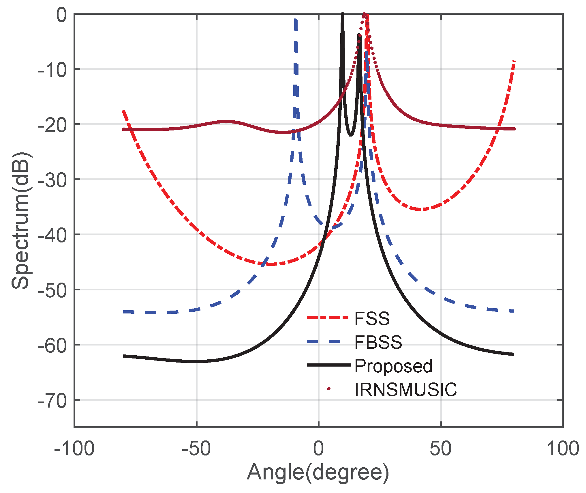
From Figure 13, it can be seen that there was only one signal trajectory in the target-orientation-course charts of the FSS algorithm and the IRNSMUSIC algorithm, and the two methods could not estimate the two coherent signals; there were two clear signal trajectories in the target-orientation-course charts of the FBSS algorithm, but the processing results of these two methods were greatly different from the actual incident angle, and the estimation results were not accurate. The two signal trajectories in the target-orientation-course charts of the proposed method were clear, the background depth was the lowest, and the estimation result was very close to the real angle. Taking the data of the 60th frame as an example, the calculated spatial spectrum is shown in Figure 14. It can be seen from Figure 14 that the proposed method could accurately estimate the incident angle of two coherent signals and that the sidelobe was the lowest. Therefore, the proposed method has the best decoherence performance and the best robustness.
The experimental results on the lake show that the proposed method has the strongest noise-suppression ability, can accurately estimate the incident angle of two coherent signals, and has the best DOA-estimation performance. It has high robustness in an actual underwater environment and has good engineering application value.
7. Conclusions
In this paper, a coherent DOA-estimation method based on an improved spatial-smoothing technique is proposed. This method directly smooths the signal subspace and uses a single-subarray-autocorrelation covariance matrix and different subarray cross-correlation covariance matrices to improve the utilization of the array receiving data. Compared to the traditional decorrelation processing method, the proposed method uses the array to receive more sufficient data information and has stronger decoherence ability. The results of simulation and lake-test data processing show that the improved method has better azimuth-estimation performance and spatial resolution. The advantages are more prominent in the case of low SNR, few snapshots, and a small signal-incident separation angle. It has good robustness in the actual underwater environment and has great engineering application value.
Author Contributions
All the authors made significant contributions to this paper. Conceptualization, Y.H.; methodology, Y.H.; formal analysis, Y.H. and X.W.; writing—original draft preparation, Y.H. and L.D.; writing—review and editing, X.W. and X.J.; validation Q.Z. All authors have read and agreed to the published version of the manuscript.
Funding
This work was funded in part by the National Natural Science Foundation of China under Grant 62171247 and in part by the Shandong Provincial Natural Science Foundation of China under Grants ZR2022MF273 and ZR2021QF113.
Data Availability Statement
Data are contained within the article.
Conflicts of Interest
The authors declare no conflicts of interest.
References
- Fu, W.; Liu, H.; Chen, Z.; Yang, S.; Hu, Y.; Wen, F. Improved Amplitude-Phase Calibration Method of Nonlinear Array for Wide-Beam High-Frequency Surface Wave Radar. Remote Sens. 2023, 15, 4405. [Google Scholar] [CrossRef]
- Zhao, A.; Ma, L.; Ma, X.; Hui, J. An improved azimuth angle estimation method with a single acoustic vector sensor based on an active sonar detection system. Sensors 2017, 17, 412. [Google Scholar] [CrossRef] [PubMed]
- Li, Y.; Shu, F.; Hu, J.; Yan, S.; Song, H.; Zhu, W.; Tian, D.; Song, Y.; Wang, J. Machine Learning Methods for Inferring the Number of UAV Emitters via Massive MIMO Receive Array. Drones 2023, 7, 256. [Google Scholar] [CrossRef]
- Schmidt, R. Multiple emitter location and signal parameter estimation. IEEE Trans. Antennas Propag. 1986, 34, 276–280. [Google Scholar] [CrossRef]
- Roy, R.H., III; Kailath, T. ESPRIT—Estimation of signal parameters via rotational invariance techniques. Opt. Eng. 1990, 29, 296–313. [Google Scholar] [CrossRef]
- Jeong, S.H.; Son, B.K.; Lee, J.H. Asymptotic performance analysis of the MUSIC algorithm for direction-of-arrival estimation. Appl. Sci. 2020, 10, 2063. [Google Scholar] [CrossRef]
- Hu, B.; Li, X.J.; Chong, P.H.J. Denoised modified incoherent signal subspace method for DOA of coherent signals. In Proceedings of the 2018 IEEE Asia-Pacific Conference on Antennas and Propagation (APCAP), Auckland, New Zealand, 5–8 August 2018; pp. 539–540. [Google Scholar] [CrossRef]
- Zhang, W.; Han, Y.; Jin, M.; Qiao, X. Multiple-Toeplitz matrices reconstruction algorithm for DOA estimation of coherent signals. IEEE Access 2019, 7, 49504–49512. [Google Scholar] [CrossRef]
- Qian, C.; Huang, L.; Zeng, W.J.; So, H.C. Direction-of-arrival estimation for coherent signals without knowledge of source number. IEEE Sens. J. 2014, 14, 3267–3273. [Google Scholar] [CrossRef]
- Han, F.M.; Zhang, X.D. An ESPRIT-like algorithm for coherent DOA estimation. IEEE Antennas Wirel. Propag. Lett. 2005, 4, 443–446. [Google Scholar] [CrossRef]
- Qi, B. DOA estimation of the coherent signals using beamspace matrix reconstruction. Signal Process. 2022, 191, 108349. [Google Scholar] [CrossRef]
- Sun, Z.G.; Bai, Q.S.; Bai, Y.Z.; Sun, R.C. Improved Weighted Spatial Smoothing Algorithm Based on Virtual Array Expansion. Syst. Eng. Electron. 2023, 45, 250–256. Available online: https://www.sys-ele.com/CN/Y2023/V45/I1/250 (accessed on 11 July 2023).
- Wen, J.; Liao, B.; Guo, C. Spatial smoothing based methods for direction-of-arrival estimation of coherent signals in nonuniform noise. Digit. Signal Process. 2017, 67, 116–122. [Google Scholar] [CrossRef]
- Li, H.S.; Shan, L.; ZHou, T. DOA estimation based on spatial smoothing for multi-beam bathymetric sonar coherent distributed sources. J. Vib. Shock 2014, 33, 138–142. [Google Scholar] [CrossRef]
- Tan, J.; Nie, Z.; Peng, S. Quadratic Forward/Backward Spatial Smoothing Polarization Smoothing MUSIC algorithm for Low Angle Estimation. In Proceedings of the 2019 IEEE Radar Conference (RadarConf), Boston, MA, USA, 22–26 April 2019; pp. 1–6. [Google Scholar] [CrossRef]
- Qi, B.; Liu, D. An enhanced spatial smoothing algorithm for coherent signals DOA estimation. Eng. Comput. 2022, 39, 574–586. [Google Scholar] [CrossRef]
- Wang, Y.; Wang, L.; Yang, X.; Xie, J.; Ng, B.W.H.; Zhang, P. Efficient cumulant-based methods for joint angle and frequency estimation using spatial-temporal smoothing. Electronics 2019, 8, 82. [Google Scholar] [CrossRef]
- Pillai, S.U.; Kwon, B.H. Forward/backward spatial smoothing techniques for coherent signal identification. IEEE Trans. Acoust. Speech Signal Process. 1989, 37, 8–15. [Google Scholar] [CrossRef]
- Dong, M.; Zhang, S.; Wu, X.; Zhang, H. A high resolution spatial smoothing algorithm. In Proceedings of the 2007 International Symposium on Microwave, Antenna, Propagation and EMC Technologies for Wireless Communications, Hangzhou, China, 16–17 August 2007; pp. 1031–1034. [Google Scholar] [CrossRef]
- Liu, Y.; Xia, X.G.; Liu, H.; Nguyen, A.H.; Khong, A.W. Iterative implementation method for robust target localization in a mixed interference environment. IEEE Trans. Geosci. Remote Sens. 2021, 60, 1–13. [Google Scholar] [CrossRef]
- Zamani, H.; Zayyani, H.; Marvasti, F. An iterative dictionary learning-based algorithm for DOA estimation. IEEE Commun. Lett. 2016, 20, 1784–1787. [Google Scholar] [CrossRef]
- Shi, Y.W.; Chen, M.; Shan, Z.T.; Shi, Y.R.; Shan, Z.B. Spatial smoothing technique for coherent signal DOA estimation based on eigen space MUSIC algorithm. J. Jilin Univ. (Eng. Technol. Ed.) 2017, 47, 268–273. [Google Scholar] [CrossRef]
- Zhang, S.; Xu, F.H.; She, L.H.; Ping-Fan, L. DOA estimation of coherent signals based on reconstructed noise subspace. J. Northeast. Univ. (Nat. Sci.) 2021, 42, 1696–1700. [Google Scholar] [CrossRef]
- Stoica, P.; Larsson, E.G.; Gershman, A.B. The stochastic CRB for array processing: A textbook derivation. IEEE Signal Process. Lett. 2001, 8, 148–150. [Google Scholar] [CrossRef]
Figure 1.
Spatial-smoothing diagram.

Figure 2.
, .

Figure 3.
, .

Figure 4.
Separation angle of the incident signal is small.
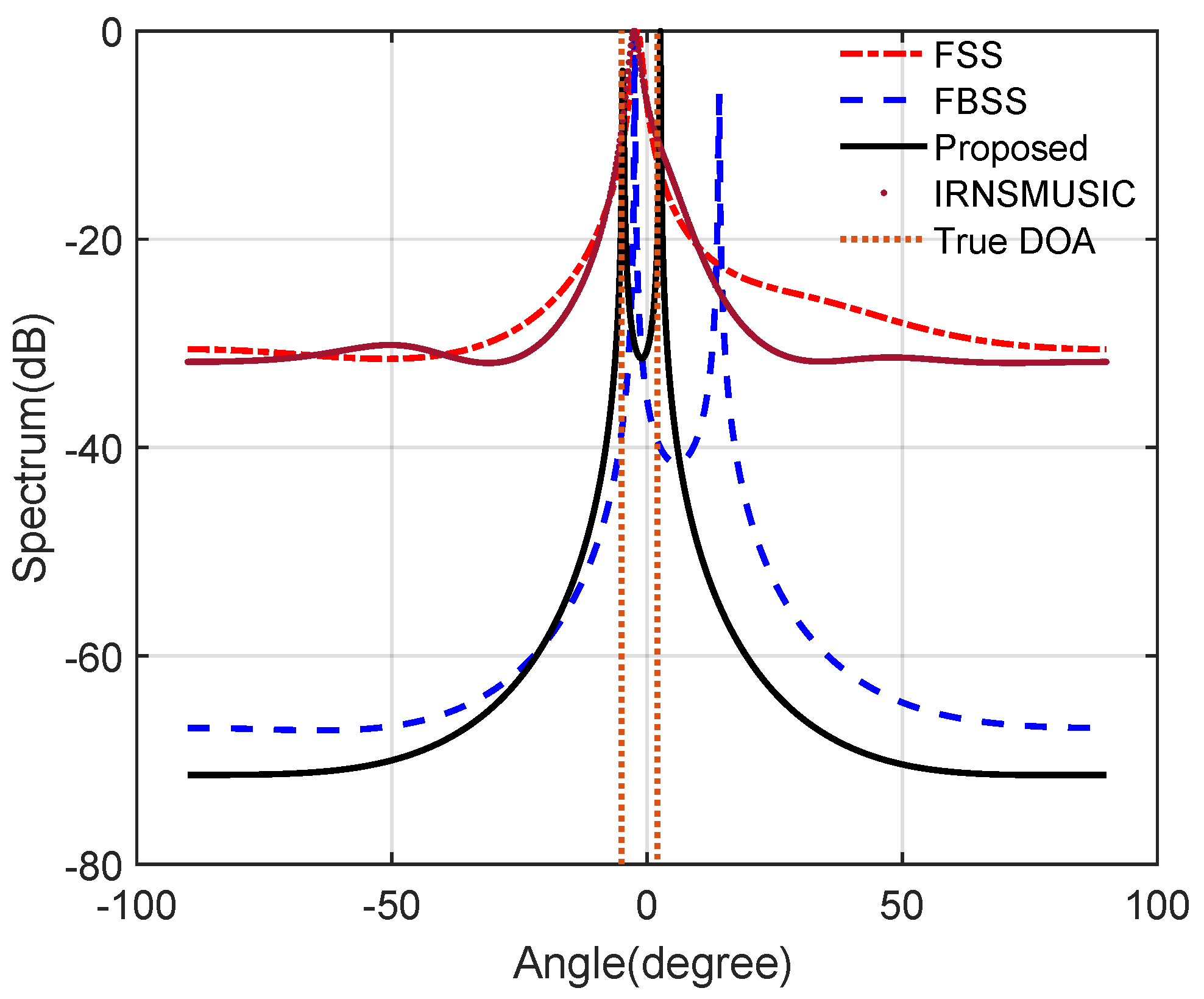
Figure 5.
RMSE of DOA estimation versus SNR.
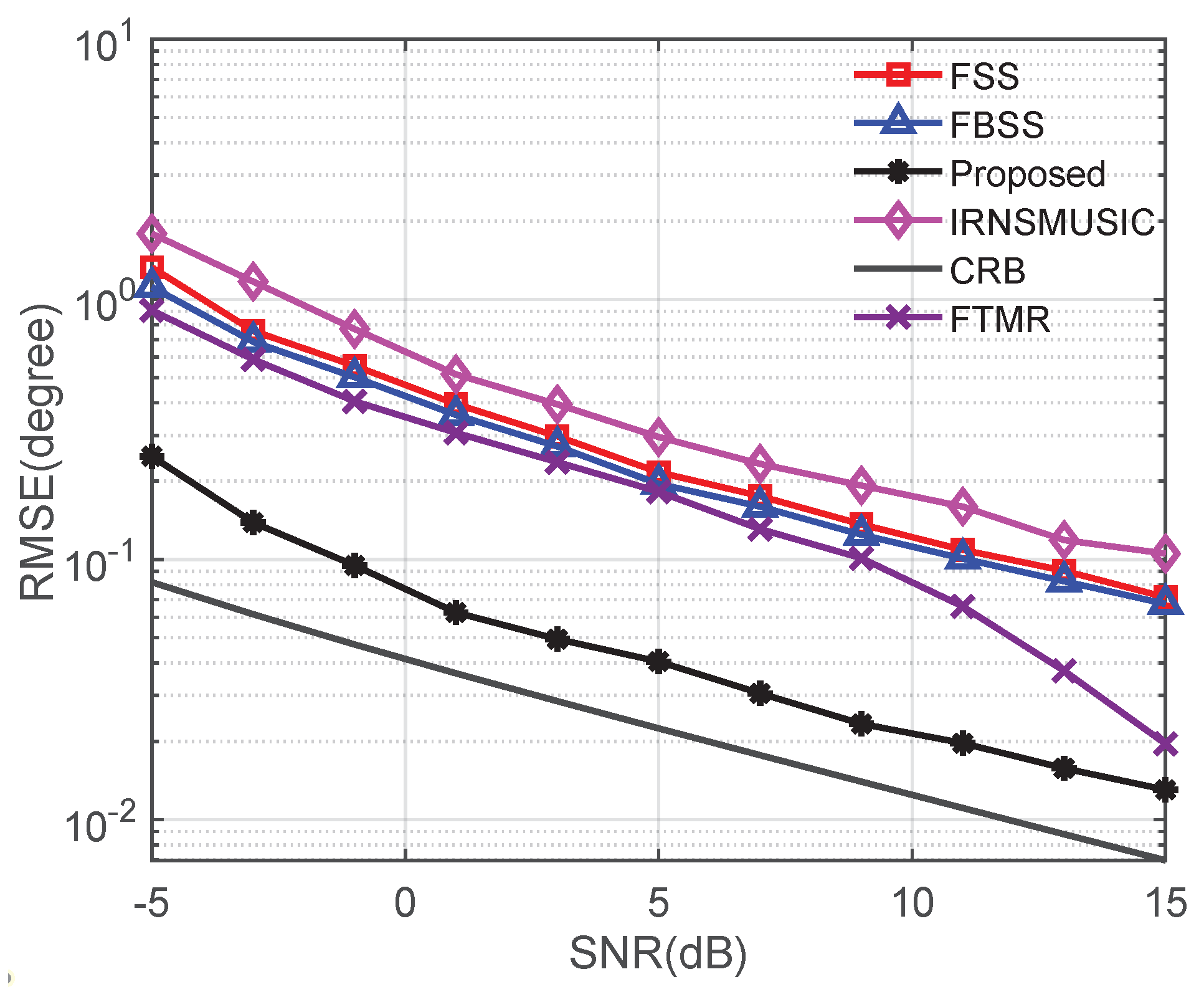
Figure 6.
Probability of resolution of DOA estimation versus SNR.
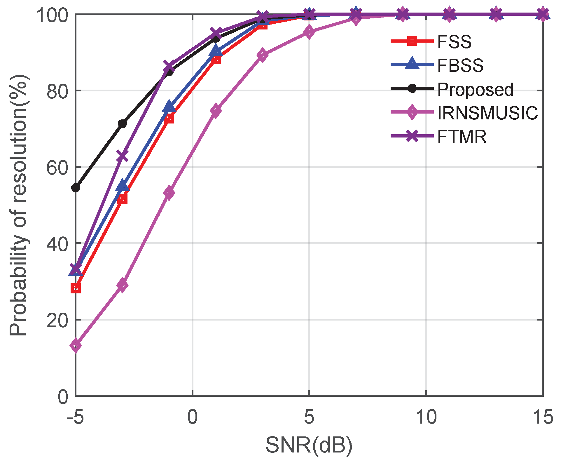
Figure 7.
RMSE of DOA estimation versus the number of snapshots.

Figure 8.
Probability of resolution of DOA estimation versus the number of snapshots.

Figure 9.
RMSE of DOA estimation versus separation angle.

Figure 10.
Probability of resolution of DOA estimation versus separation angle.
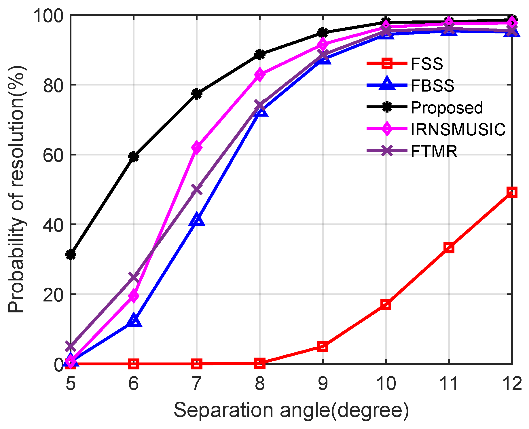
Figure 11.
Schematic diagram of equipment layout.
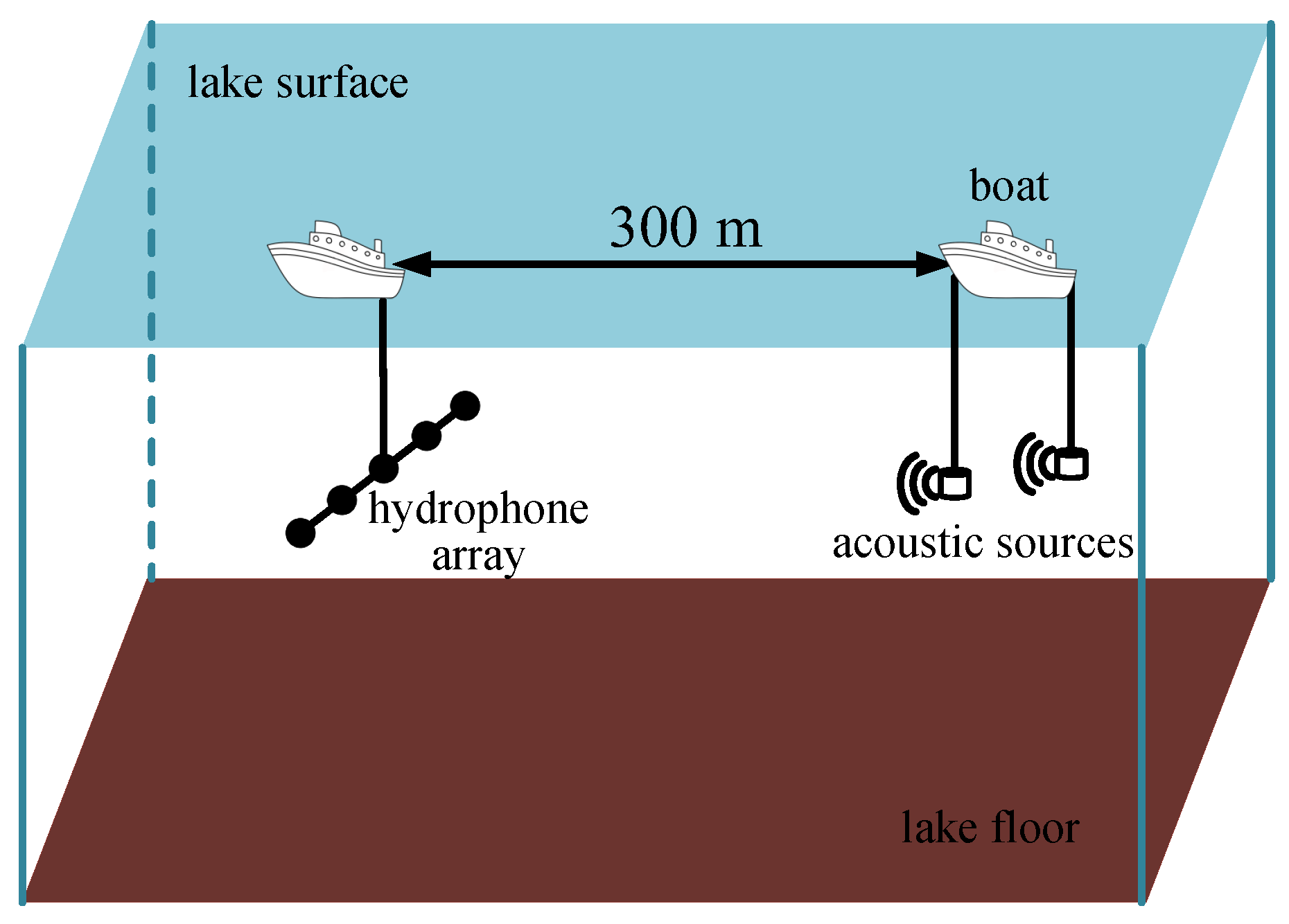
Figure 12.
The actual data received by the array.
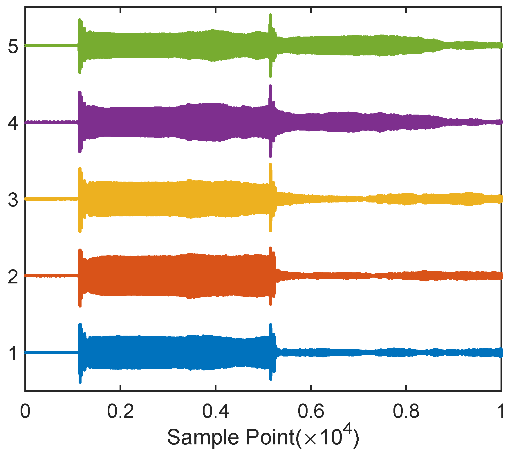
Figure 13.
Target−orientation-course charts obtained by four algorithms: (a) proposed; (b) FSS; (c) FBSS; (d) IRNSMUSIC.
Figure 13.
Target−orientation-course charts obtained by four algorithms: (a) proposed; (b) FSS; (c) FBSS; (d) IRNSMUSIC.
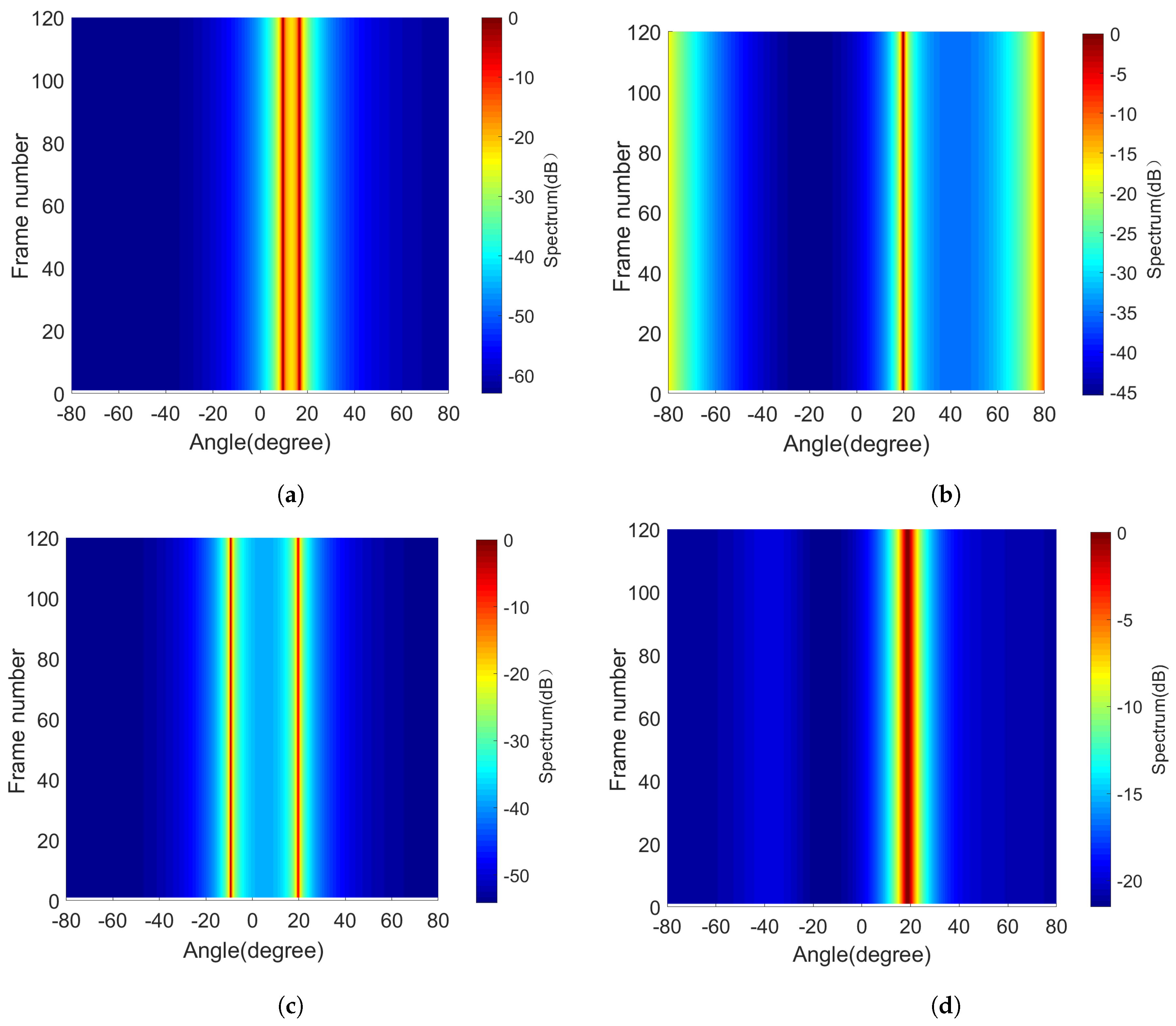
Figure 14.
Spatial spectrum of 60th frame data.
Disclaimer/Publisher’s Note: The statements, opinions and data contained in all publications are solely those of the individual author(s) and contributor(s) and not of MDPI and/or the editor(s). MDPI and/or the editor(s) disclaim responsibility for any injury to people or property resulting from any ideas, methods, instructions or products referred to in the content. |
© 2023 by the authors. Licensee MDPI, Basel, Switzerland. This article is an open access article distributed under the terms and conditions of the Creative Commons Attribution (CC BY) license (https://creativecommons.org/licenses/by/4.0/).
Share and Cite
MDPI and ACS Style
Hou, Y.; Wang, X.; Ding, L.; Jin, X.; Zhang, Q. DOA-Estimation Method Based on Improved Spatial-Smoothing Technique. Mathematics 2024, 12, 45. https://doi.org/10.3390/math12010045
AMA Style
Hou Y, Wang X, Ding L, Jin X, Zhang Q. DOA-Estimation Method Based on Improved Spatial-Smoothing Technique. Mathematics. 2024; 12(1):45. https://doi.org/10.3390/math12010045
Chicago/Turabian StyleHou, Yujun, Xuhu Wang, Lei Ding, Xu Jin, and Qunfei Zhang. 2024. "DOA-Estimation Method Based on Improved Spatial-Smoothing Technique" Mathematics 12, no. 1: 45. https://doi.org/10.3390/math12010045
Note that from the first issue of 2016, this journal uses article numbers instead of page numbers. See further details here.