Machine Learning Techniques Applied to the Harmonic Analysis of Railway Power Supply

Abstract

Harmonic generation in power system networks presents significant issues that arise in power utilities. This paper describes a machine learning technique that was used to conduct a research study on the harmonic analysis of railway power stations. The research was an investigation of a time series whose values represented the total harmonic distortion (THD) for the electric current. This study was based on information collected at a railway power station. In an electrified substation, measurements of currents and voltages were made during a certain interval of time. From electric current values, the THD was calculated using a fast Fourier transform analysis (FFT) and the results were used to train an adaptive ANN—GMDH (artificial neural network–group method of data handling) algorithm. Following the training, a prediction model was created, the performance of which was investigated in this study. The model was based on the ANN—GMDH method and was developed for the prediction of the THD. The performance of this model was studied based on its parameters. The model’s performance was evaluated using the regression coefficient (R), root-mean-square error (RMSE), and mean absolute error (MAE). The model’s performance was very good, with an RMSE (root-mean-square error) value of less than 0.01 and a regression coefficient value higher than 0.99. Another conclusion from our research was that the model also performed very well in terms of the training time (calculation speed).

1. Introduction

Nowadays, transportation is becoming increasingly reliant on electricity. Railway transport, in particular, is over 90% electrified. At the moment, transportation is critical. In general, all forms of transportation emit some level of pollution. However, when compared with other types of transportation, railway transportation may be the least polluting because it uses electricity. Transport on electrified railways is advantageous because it allows for relatively fast travel, ensures sustainability, and reduces pollution [1,2,3]. However, there are some issues with electrified rail transportation that affect power quality. Reactive power and harmonic currents are examples of these [4,5].

A perfect power supply is always accessible, operates within permissible voltage and frequency limits, and has a perfectly sinusoidal voltage curve. Poor-quality voltage is a hidden expense. Usually, it goes unreported and misdiagnosed as long as there are no costly failures. The effect of nonlinear equipment on power quality is proportional to the nominal power [6,7]; computers and printers, fluorescent lighting, battery chargers, and variable-speed drives are among examples of this.

Load types in power systems have changed significantly in recent decades, with an increase in the number and variety of nonlinear loads. Any load with a nonlinear V–I characteristic produces current harmonics in the electrical network [8]. Rectifiers with thyristors used to control the train speed in railway transportation cause harmonic distortion of the current due to their nonlinear characteristic [2]. These harmonics have an effect on the power quality and cause power loss. Harmonics were shown to reduce the power factor by 1–5% [8]. Inter-harmonics appear, particularly in electric rail. The inter-harmonics are non-integer multiples of the power system’s frequency components up to 2 kHz. Even at low amplitude levels, the presence of inter-harmonics can cause additional problems, such as sub-synchronous oscillations, light flickers, and voltage fluctuations [9].

Numerous studies were conducted in order to eliminate, or at least reduce, the harmonics of the current and, implicitly, the voltage [10,11].

Current harmonics are becoming more prevalent due to the increased usage of nonlinear electrical equipment in numerous industries, including rail transportation [4,5,8,9]. Modern electrical and electronic equipment, including home appliances, consists primarily of switching sources [7].

2. Related Works

In this section, we present previous research that is the most relevant to our work in a concise manner. The research presented here aimed to investigate the impact of electrified railway transportation on power quality.

There was a considerable amount of research done on the power quality of railway transportation.

The paper [1] emphasizes the main effects that electric locomotives produce: harmonic currents, reactive power, and unbalanced currents, which can cause unbalanced voltages. The research was based on measurements from the 25 kV Electric Railway System.

A system of harmonics filters (both DC and AC) was proposed in article [5], which focuses on the research of current harmonics in railway substations, which were tested via simulation in Matlab, achieving a reduction of these harmonics by 5% below the IEEE requirements. Furthermore, in [2], hybrid reactive power filters composed of active and passive filters were used to reduce current harmonics and compensate for reactive power in a railway substation. A model in Matlab Simulink was also proposed for analyzing the effects of these filters and compensators.

In their article [4], the authors described a methodology for achieving optimal filter design for harmonic filtration in railway substations across the full spectrum of harmonic frequencies. Measurements are presented in the work that highlighted the presence of harmonics (particularly those of low order) in a substation railway. The described method was used to design the filters and was validated through simulation.

The goal of the work in [8] was to investigate power quality in railway substations. PQ was analyzed for various types of transformer stations, with simulations for each type highlighting the harmonics that occurred in each case.

The study of current harmonics produced by non-linear electrical loads was carried out using various methods in the specialized literature because it is useful to understand as much as possible about their values in order to have a strategy to reduce them, both in the short and long terms.

As evidenced by studies [12,13,14] in 2007, [15] in 2008, [16] in 2013, [17] in 2015, [18] in 2016, [19,20] in 2017, [21] in 2018, [22] in 2019, [23,24] in 2020, [25] in 2021, and [26,27] in 2022, the monitoring, tracking, and prediction of current harmonics began in the last few decades. The prediction of the power factor in 2022 was also discussed in article [28], which is considered to be a significant indicator of power quality. All of these research studies focused on THD prediction by applying intelligent methods, and the preponderance of them was based on intelligent methods and ANN.

According to the results presented in papers [12,13,14,15], ANN models are capable of producing reliable estimates of the voltage THD, current THD, and power factor.

A method for harmonic current prediction based on EMD-SVR (empirical mode decomposition–intrinsic mode regression) theory and applied to forecasting is proposed in article [16]. Article [17] also addresses harmonic current prediction using a double Fourier series analysis to eliminate high-frequency harmonics from all harmonic contents.

Comparisons between measured and predicted results were made in article [18]. These comparisons demonstrate that the method used in this study was effective and can be used as a model to predict the RMS value of the current and THD.

The authors of [20,21] proposed a method for short-term harmonic forecasting from electrified railways on the power grid using a stack autoencoder (SAE) neural network. Among the conclusions of these studies is the importance of short-term predictions of harmonics that affect the railways’ electric power supply network.

Total harmonic distortion (THD) prediction (in a grid-connected photovoltaic system) is illustrated in the study [22] using a heuristic algorithm called grey wolf optimizer–least-squares support vector machine.

The paper [23] illustrates a technique for THD prediction based on a hybridized heuristic algorithm called grey wolf optimizer–least-squares support vector machine (GWO-LSSVM). The authors of [23] concluded that their proposed method performed well when compared with other methods.

Based on ANN-Narx and utilizing Matlab/Simulink for distribution system modeling and simulation, the paper [24] presents a multi-step prediction technique for THD in networks with nonlinear loads. The research [24] investigated the proposed prediction method on three distinct nonlinear loads using the distribution system to demonstrate its applicability.

The article [26] focuses on a THD prediction method based on an improved AdaBoost algorithm that employs a generalized regression neural network (GRNN). The mind evolution algorithm optimizes the GRNN, which is trained and simulated using the experiment’s harmonic data.

Prediction methods for voltage THD at low-voltage bus bars are also proposed in the paper [27]. Prediction techniques for THD involving autoregressive and feedforward neural networks are explored in [27].

The research presented in the paper [28] utilized sequential artificial neural networks (ANNs) for the accurate estimation of harmonic distortion in large transmission networks. The authors highlighted the benefits of their method in terms of the THD estimation accuracy it provided.

The article [29] titled “Review of AI applications in harmonic analysis in power systems” discusses in a very comprehensive manner how artificial intelligence (AI) techniques are used in numerous perspectives of analyzing harmonics in electrical power.

Our study was also focused on THD modeling and prediction using experimental measurements via new machine learning techniques. The method used in this study was a novel technique with better performances than the classical ANN. Experiments were carried out in a Romanian substation to analyze this power quality in order to apply this technique, which was based on ANN-GMDH. Following these experiments, the total harmonic distortion of the current and voltage in the power supply substation was calculated and found to be high.

Many recent studies focused on the application of new machine learning techniques in the modeling, prediction, and forecasting of nonlinear systems.

Short-term power load forecasting can ensure power grid safety and stability in a short period. The paper [30] describes an attention bidirectional LSTM (long short-term memory) system that was used for power load forecasting. The same LSTM-based technique was used in the study [31] to reduce power fluctuations in an islanded microgrid.

Furthermore, many studies [32,33,34,35] investigated the problem of power load forecasting using a modeling technique based on LSTM.

Machine learning is a popular method for extracting useful and optimal features from data to improve classification performance. As a result, the study [36] employed a machine learning technique for analyzing and identifying power quality disturbances. The study presented in [36] employed an LSTM model to identify various power quality disturbances, such as voltage sag, voltage swell, interruption, impact, oscillation, and harmonics. These disruptions were both simulated and validated. In addition, to classify power quality disturbances, the study [37] employed a hybrid model of multi-resolution analysis and a long short-term memory network.

In numerous studies, machine learning and, more recently, deep learning techniques were found to be effective at analyzing power quality and harmonics. The article [38] proposes a fault detection method for harmonic reducers based on the CNN-LSTM (convolutional neural network–LSTM) model. Hybrid research using ANN and deep learning to improve forecasting in order to study the possibilities of improving power quality, developing load forecasting models to study power consumption, and fault detection. Forecasting techniques are affected by various sources of randomness. Improvements to prediction models with more accurate results and lower errors are required. The article [39] presents and compares an innovative short-term forecasting system based on GMDH to the LS-SVM (least-squares support vector machine).

The prediction of time series has significant theoretical implications and numerous engineering applications [40]. Forecasting can be used in applications where estimation is not possible [39,40,41,42]; it is the process of determining future values of time series data based solely on past data. Because of its wide range of applications, time series forecasting is a current research topic [32,33,34,35,36].

There are several methods for forecasting time series. ANN-based methods were shown to benefit nonlinear time series forecasting [43,44].

GMDH is an effective modeling and prediction tool [45,46]. This study employed an ANN based on GMDH to model and predict total harmonic distortion in railway power supplies in the short term.

3. Materials and Methods

The measurements made in a railway power supply station were used to perform the harmonics analysis. The voltage and current in a single phase were measured. An FFT was also used to calculate the values of the current and voltage harmonics [47]. Fourier analysis is the process of converting a time wave signal into a frequency or spectrum component. There are numerous methods for converting the time domain of a sampling signal to its frequency domain, but the fast Fourier transformation (FFT) is the most well-known.

Figure 1 depicts the electrical scheme used to collect the measurements. The measurements were made on the single phase in the secondary of the substation transformer. Because the use of an electric locomotive, which is connected to the secondary of the transformer, is the primary source of pollution in the railway power supply system, electromagnetic pollution is at its peak in this area, which is why this measurement point was chosen. The second reason for choosing this measurement point was that the transformer used a current and voltage symmetrization scheme, which improved the electrical parameters of the transformer’s primary connection.

The instantaneous current and voltage values were measured using an NI MyRIO data acquisition board at a 5 kHz acquisition frequency.

Figure 2 depicts the variation in current and voltage, which was distorted and did not have a perfectly sinusoidal variation.

To quantify harmonic distortions, the total harmonic distortion index was calculated using Formula (1).

$$THDI=\frac{\sqrt{{{\displaystyle \sum }}_{k=2}^{\infty }{\left(I_k\right)}^2}}{I_1},$$

(1)

A total of 40 harmonics were used because the values of the harmonics were insignificant above this value.

Figure 3 depicts the current and voltage harmonics of the waveform depicted in Figure 2. These values were obtained through the use of an FFT. These harmonics had excessively high values, particularly in the case of the current harmonics.

As shown in Figure 3, the harmonics of even order had higher values than harmonics of odd order, as expected.

The THD values of the current were determined over a longer time in order to make a complete and consistent analysis of the variation of the total harmonic distortion. For this, data was recorded at a frequency of 5 kHz, and the THD frequencies of the current were calculated using this data. Figure 4 depicts this. This determination was made for a time interval of approximately 16 min. Every 1 s, a sample was calculated. The THD varied significantly depending on several factors.

To investigate the power quality, modeling, and forecasting were performed using an adaptive ANN—GMDH for THDI.

3.1. GMDH

The group method of data handling (GMDH) is a set of inductive algorithms that are used to mathematically model datasets.

Applications of GMDH include data mining, prediction, modeling of complex systems, optimization, and pattern recognition [48]. This methodology is also known as a polynomial neural network, which is a machine learning method. The GMDH is a meta-heuristic method that can be utilized in conjunction with other techniques, such as genetic algorithms, particle swarm optimization algorithms, the fuzzy method, backpropagation, and the Levenberg–Marquardt method [49].

The method operates by dividing the problem model into simple patterns and then reassembling them using a pre-selection.

A GMDH network that has n inputs but only one output is considered to be a subset of the components of the base function, which may be found in (2) ([48]).

$$Y\left(x_1, x_2,\dots , x_n\right)=a_0+{{\displaystyle \sum }}_{i=1}^m{a}_i{f}_i,$$

(2)

In Equation (2), f denotes the elementary functions that depend on different sets of inputs, a_i denotes the coefficients, and m denotes the number of base function components.

Several subsets of the base function (2) that represent partial models are evaluated by GMDH algorithms in order to determine which one produces the optimal answer. These models’ coefficients are estimated using the least-squares method. GMDH algorithms progressively increase the number of partial model components until a model structure with the smallest value of an external criterion is identified. The concept for this is model self-organization.

In fact, a GMDH is a model of self-organizing neural networks. The equation that describes the relationship between the inputs and outputs in a GMDH model may be seen in Equation (3) [48].

$$y=a_0+{{\displaystyle \sum }}_{i=1}^m{a}_i{x}_i+{{\displaystyle \sum }}_{i=1}^m{{\displaystyle \sum }}_{j=1}^m{a}_{ij}{x}_i{x}_j+{{\displaystyle \sum }}_{i=1}^m{{\displaystyle \sum }}_{j=1}^m{{\displaystyle \sum }}_{k=1}^m{a}_{ijk}{x}_i{x}_j{x}_k+\cdots ,$$

(3)

where the inputs are x_i, i = 1, …, m; the polynomial coefficients are a_ijk, with i, j, k = 1, …, m; and the output is y.

A typical GMDH training model is depicted in Figure 5. The nodes in the input layer stand in for the network’s input values, while the nodes in the hidden layer and the output layer stand in for the neurons.

3.2. Training ANN—GMDH

GMDH ANNs are modelling techniques that are based on learning relationships between input variables. A GMDH is also used in time series forecasting. In this case, the algorithm uses values at delayed time points as inputs [46].

The following steps are used to train the polynomial networks ANN—GMDH.

An initial layer is created, as with MLP (multi-layer perceptron) networks. The first layer is created by the algorithm based on the number of inputs representing partial descriptions. The number of nodes is defined as m two-by-two network entry combinations ($m=C_n^2$) [49]. Each first-layer neuron output is dependent on two inputs, as is shown in (4) [48].

$$y_{1i}=f_{1i}\left(x_j,x_k\right), i=1,\dots m; j,k=1,\dots ,n,$$

(4)

The neurons in this layer are trained, and neurons that fail to meet the minimum requirements are eliminated after training. After calculating the coefficients, the algorithm evaluates the performance and eliminates the neurons with the worst results. A method is used to evaluate the performance of a neuron that is based on an imposed minimum error defined by Equation (5) [50].

$$e_c=\alpha \times RMS{E}_{min}+\left(1-\alpha \right)\times RMS{E}_{max},$$

(5)

In Equation (5), α is a selection-pressure-influencing coefficient, and RMSE_min and RMSE_max are the root-mean-square minimum and maximum values, respectively [50].

The training process is depicted as a logical diagram in Figure 6. Figure 7 depicts an example of the GMDH ANN architecture with four inputs and three layers. Low-performance nodes are colored lighter in Figure 7 and removed. When the last layer has a single node, the training stops.

3.3. Modeling the Total Harmonic Distortion with ANN—GMDH

In the rail power supply station, a model incorporating GMDH and experimental measurements was developed. A GMDH was used to model and analyze the power quality using total harmonic distortions. The values of the THDI at time-delayed moments were put into a vector that were used as inputs for the ANN to create the time series that were used in ANN-GMDH training.

If the time series has t time points and m inputs, the m inputs represent previous total harmonic distortion samples that were used in the input layer.

A total of m nodes representing previous samples of total harmonic distortion were used in the input layer of the case presented in this paper.

Figure 8 depicts the development of the first layer of a GMDH network for the modeling and prediction of a time series. For m = 4, an example of THDI variation was used.

The following gives three well-known measures that were used to evaluate the performance of the ANN—GMDH modeling. These measures are described as follows [51]: the regression coefficient (R), root-mean-square error (RMSE), and mean absolute error (MAE, MSE), as shown in Equations (6)–(8).

$$MSE=\frac{{{\displaystyle \sum }}_{i=1}^n\left(y_m-\overline{y_m}\right)\left(y_p-\overline{y_p}\right)}{{{\displaystyle \sum }}_{i=1}^n{\left(y_m-\overline{y_m}\right)}^2{{\displaystyle \sum }}_{i=1}^n{\left(y_p-\overline{y_p}\right)}^2}$$

(6)

$$RMSE=\sqrt{\frac{1}{n}{\displaystyle \sum }_{i=1}^n{\left(y_m-y_p\right)}^2}$$

(7)

$$MAE=\frac{1}{n}{\displaystyle \sum }_{i=1}^n\left|y_m-y_p\right|$$

(8)

where y_p and y_m are, respectively, the predicted THD and measured THD; n is the number of measured data; and $\overline{y_p}$ and $\overline{y_m}$ are the average value of predicted THD and measured THD, respectively.

Root-mean-square error (RMSE): This is a statistical measure of precision that has many applications in engineering experiments. The RMSE is scale-dependent and is used to compare errors in various numerical models. Specifically, the RMSE detects differences between predicted and observed values.

Another parameter determined was the error standard deviation, which is shown in (9).

$$S=\sqrt{\frac{1}{N-1}{\displaystyle \sum }_{i=1}^N{\left|E_i-\mu \right|}^2}$$

(9)

where μ is the mean of E, the errors:

$$\mu =\frac{1}{N}{\displaystyle \sum }_{i=1}^N{E}_i$$

(10)

4. Results

A model incorporating the GMDH and the experimental THDI measurements was created. The model was used for the GMDH ANN training with the values of the THDI at time-delayed moments. In fact, the THDI samples represented in Figure 3 were used for training, as shown in Figure 6. Matlab was used to create the simulations, which were then compared with the experimental measurements. The following network parameters were used to train the GMDH ANN:

• The percentage of training data, pTrain;
• The maximum number of neurons accepted per layer, nMax;
• The maximum number of layers, maxL;
• The m value, which represents the number of previous samples used for prediction;
• A layer’s selection pressure, α.

As a result, the model was created and tested in Matlab using the flowchart of the GMDH algorithm shown in Figure 9.

Matlab and the Neural Network Toolbox were used to create the model. The experiments were carried out by varying the model’s parameters within certain limits. For the percentage of training data, for example, values between 60% and 80% were considered. The maximum number of neurons on each layer is a variable with fairly broad limits. In the study presented in this paper, values ranging from 3 to 50 were considered. It is obvious that having too few neurons on a layer does not provide adequate model performance or accuracy. A large number of neurons on a layer, on the other hand, results in too many calculations and does not significantly improve the model’s performance. In contrast, high values of this parameter result in very good training data performance but poor test data performance, leading to the conclusion that the model lost its ability to generalize.

The maximum number of layers is another parameter that can be considered. Many layers can theoretically be introduced, but experiments show that increasing the number of layers too much does not always result in better model performance. It also achieves good performance on training data while performing poorly on test data. Experiments were also conducted in which the number of previous samples used to predict the next sample was varied. The conclusion was that increasing the number of previous samples improved the model performance, but a large increase in the number of previous samples was not justified because the calculation was too complicated and a much higher accuracy was not obtained. Because the model had many parameters, it was obvious that determining a unique optimal configuration of the model was difficult, as there were several configurations that offered very good performance. Following the experiments, we selected a configuration that provided good model accuracy on both the training and test data. The results from Figure 10, Figure 11, Figure 12 and Figure 13 are presented for this configuration.

Figure 10 depicts the THDI (a) and errors (b) variations obtained with this model using the training data for the following parameters: nMax = 16, maxL = 6, α = 0.5, m = 5, and pTrain = 70%. Figure 11 depicts the error mean and the error standard deviation for the same parameters as in Figure 10.

Figure 12 depicts the THDI (a) and errors (b) variations obtained with this model using the testing data for the following parameters: nMax = 16, maxL = 6, α = 0.5, m = 5, and pTrain = 70%. Figure 13 depicts the error mean and the error standard deviation for the same parameters as in Figure 12.

5. Discussion

The model’s parameters were chosen after several experiments, which revealed that they provided good model performance. These parameters were obviously not unique and exhaustive. There was a range of values for which the model’s performance was otherwise satisfactory. In

Table 1. The model performances for different values of model parameters.

Model Parameters: α/maxL/nMax		Train					Test
		MSE	RMSE	Error Mean	Error Std	R	MSE	RMSE	Error Mean	Error Std	R
α = 0, maxL = 4	8	0.00019	0.01372	0.00141	0.01366	0.99938	0.00016	0.01261	0.00119	0.01257	0.99874
	12	0.00015	0.01231	−0.00192	0.01216	0.99914	0.00011	0.01056	−0.00135	0.01049	0.99909
	16	0.00014	0.01187	0.00454	0.01097	0.99939	0.00010	0.00989	0.00449	0.00882	0.99910
	20	0.00009	0.00965	0.00027	0.00966	0.99928	0.00008	0.00872	−0.00002	0.00873	0.99917
	24	0.00018	0.01330	−0.00224	0.01312	0.99926	0.00012	0.01107	−0.00222	0.01087	0.99912
α = 0.3, maxL = 4	8	0.00016	0.01265	−0.00071	0.01264	0.99915	0.00015	0.01202	−0.00018	0.01204	0.99850
	12	0.00012	0.01108	−0.00174	0.01095	0.99942	0.00013	0.01148	−0.00127	0.01143	0.99870
	16	0.00033	0.01813	0.00027	0.01815	0.99816	0.00036	0.01901	0.00084	0.01902	0.99575
	20	0.00015	0.01229	0.00047	0.01229	0.99947	0.00017	0.01320	0.00028	0.01322	0.99870
	24	0.00017	0.01312	0.00212	0.01295	0.99927	0.00013	0.01118	0.00191	0.01104	0.99906
α = 0.6, maxL = 4	8	0.00023	0.01509	0.00001	0.01510	0.99897	0.00016	0.01264	0.00099	0.01263	0.99878
	12	0.00023	0.01513	0.00221	0.01498	0.99938	0.00017	0.01299	0.00299	0.01266	0.99905
	16	0.00013	0.01156	0.00104	0.01152	0.99930	0.00012	0.01080	0.00074	0.01079	0.99885
	20	0.00008	0.00911	0.00224	0.00884	0.99975	0.00008	0.00899	0.00238	0.00868	0.99939
	24	0.00016	0.01264	−0.00106	0.01261	0.99916	0.00016	0.01262	−0.00099	0.01260	0.99838
α = 0.9, maxL = 4	8	0.00017	0.01304	0.00126	0.01299	0.99941	0.00012	0.01081	0.00189	0.01066	0.99918
	12	0.00023	0.01514	−0.00012	0.01515	0.99905	0.00018	0.01331	−0.00023	0.01333	0.99867
	16	0.00024	0.01542	0.00074	0.01541	0.99885	0.00018	0.01339	0.00146	0.01333	0.99827
	20	0.00007	0.00845	−0.00140	0.00834	0.99965	0.00008	0.00885	−0.00199	0.00863	0.99932
	24	0.00019	0.01389	−0.00100	0.01386	0.99897	0.00017	0.01293	−0.00062	0.01294	0.99904
α = 0, maxL = 6	8	0.00018	0.01325	−0.00130	0.01319	0.99912	0.00011	0.01070	−0.00108	0.01066	0.99908
	12	0.00036	0.01909	0.00161	0.01903	0.99835	0.00039	0.01975	0.00118	0.01975	0.99665
	16	0.00033	0.01804	0.00157	0.01799	0.99745	0.00050	0.02226	0.00313	0.02208	0.99312
	20	0.00016	0.01247	−0.00144	0.01239	0.99900	0.00016	0.01244	−0.00032	0.01246	0.99836
	24	0.00021	0.01441	0.00078	0.01440	0.99919	0.00015	0.01237	0.00035	0.01239	0.99889
α = 0.3, maxL = 6	8	0.00020	0.01398	0.00070	0.01397	0.99875	0.00018	0.01336	0.00155	0.01329	0.99834
	12	0.00014	0.01177	0.00303	0.01138	0.99908	0.00016	0.01273	0.00312	0.01237	0.99853
	16	0.00016	0.01599	−0.00004	0.01600	0.99808	0.00023	0.01489	−0.00282	0.01489	0.99701
	20	0.00021	0.01463	0.00188	0.01452	0.99886	0.03746	0.01935	0.00131	0.01941	0.99672
	24	0.00016	0.01278	0.00441	0.01200	0.99918	0.00014	0.01184	0.00437	0.01103	0.99878
α = 0.6, maxL = 6	8	0.00015	0.01240	−0.00139	0.01233	0.99915	0.00011	0.01052	−0.00086	0.01051	0.99903
	12	0.00020	0.01401	0.00219	0.01385	0.99921	0.00019	0.01381	0.00194	0.01370	0.99860
	16	0.00032	0.01778	0.00086	0.01777	0.99790	0.00017	0.01317	0.00138	0.01312	0.99846
	20	0.00020	0.01400	−0.00265	0.01376	0.99864	0.00015	0.01214	−0.00255	0.01189	0.99874
	24	0.00021	0.01444	−0.00116	0.01441	0.99849	0.00038	0.01948	−0.00001	0.01951	0.99508
α = 0.9, maxL = 6	8	0.00016	0.01277	0.00149	0.01269	0.99937	0.00014	0.01177	0.00183	0.01165	0.99884
	12	0.00021	0.01435	−0.00130	0.01430	0.99921	0.00019	0.01384	−0.00120	0.01381	0.99851
	16	0.00013	0.01127	0.00059	0.01126	0.99965	0.00010	0.01015	0.00129	0.01009	0.99914
	20	0.00020	0.01425	−0.00158	0.01417	0.99916	0.00016	0.01260	−0.00126	0.01256	0.99868
	24	0.00015	0.01205	0.00060	0.01204	0.99944	0.00014	0.01189	0.00103	0.01186	0.99889

, the values of the coefficients that characterized the model for several sets of its parameters were entered to give us an idea and to allow for comparative quantitative analysis. Table 1 displays the results of the ANN—GMDH modelling for various sets of model parameters, both for the training and test data. There were five previous samples.

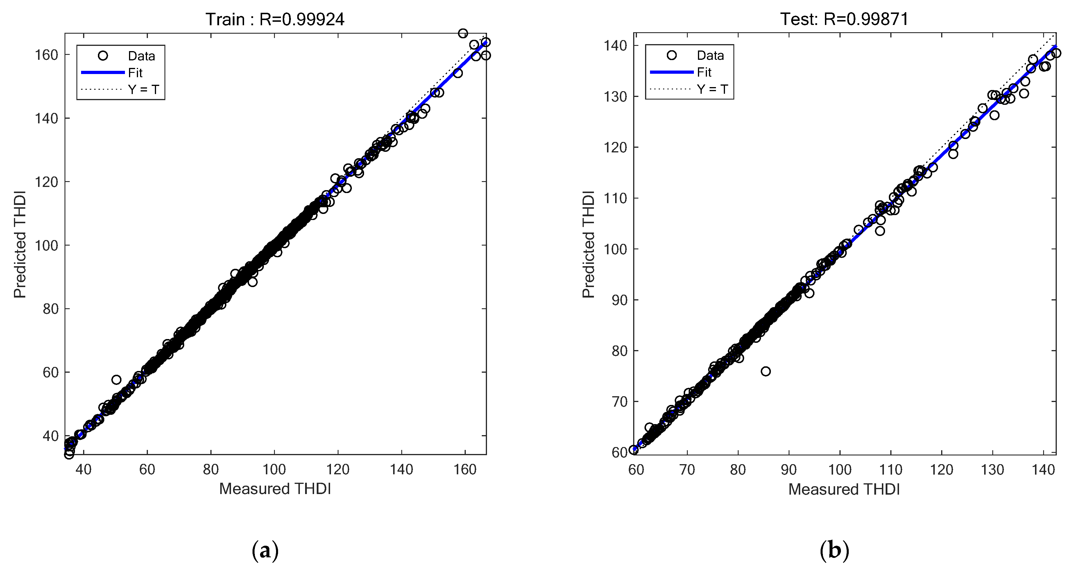
Figure 14a,b show the regression coefficients for the training and testing data, respectively.

Simulations in Matlab were carried out to study the behavior of the developed model in relation to its parameters, as shown in Figure 15 and Figure 16. The number of layers added to the adaptive GMDH ANN varied depending on the maximum number of neurons on a layer and the selection pressure. In any case, the error was acceptable, demonstrating the stability of the developed model. As can be seen, selection pressure was the most influential factor regarding the number of layers added.

As expected, at very low selection pressure, the number of layers added was the maximum of 10 imposed by the GMDH model parameters. However, when the selection pressure was increased, the maximum number of layers did not reach the limit imposed by the model parameters. The number of layers added to ANN—GMDH influenced the RMSE as well. As a result, with a small pressure selection and a large number of layers (10, which was the maximum allowed in our experiments), the RMSE error began to increase. This means that adding too many layers did not improve the model’s performance. The model provided good performance for a maximum of 4–6 layers and a selection pressure of around 0.5.

Figure 15 and Figure 16 depict the RMSE value as a function of the model parameters. Thus, in Figure 15, the RMSE value is represented as a variation in selection pressure ranging from 0 to 1 and a maximum number of neurons on a layer ranging from 10 to 50. Figure 16 depicts the RMSE as a function of selection pressure and the number of layers allowed to be added, with a maximum of 10 neurons per layer accepted.

We compared our research results with those of other studies in the literature. The paper [25] focuses on THD prediction using the AdaBoost algorithm, which was used to integrate multiple MEA-GRNNs (generalized regression neural networks). The technique was referred to as Ada-MEA-GRNN by the authors. The paper [25] compares the authors’ research results with BP, GRNN, MEA-GRNN, and Ada-MEA-GRNN algorithms, demonstrating that their method outperformed the others in terms of the RMSE, MAE, median absolute deviation, and accuracy. The same parameters were determined in our study. When we compared the parameters obtained in our study with those presented in [25], we concluded that our ANN-GMDH-based method performed better. As shown in Table 1, the maximum RMSE was 0.01 (less than 0.1483 from [25]). Furthermore, MAE was limited to 0.004 (less than the 0.03 from [25]), and the error standard deviation was limited to 0.01 (less than the 0.02 from [25]). As a result, we can say that our method performed better.

We also considered articles [20,21] in order to make comparisons with other studies. A stack autoencoder (SAE) neural network was used in the study [20] for short-term harmonic forecasting. The paper [20] highlights the importance of short-term harmonic forecasting from electrified railways on the power grid and proposes a model and method for short-term harmonic forecasting and evaluation based on a stack autoencoder neural network. The method is also based on measured data, and the harmonic forecasting relative error ranges between −10% and +10%. The article [21] compares the SAE neural network to the BP neural network, which was also used for short-term harmonic forecasting from electrified railways. The authors of [20] concluded that the BP method is also suitable for harmonic forecasting, with the relative error of harmonic forecasting based on the BP method ranging between 15% and 20%. When compared with the results of [20,21], the method used in this study performed better for harmonics forecasting.

The prediction of current harmonics produced by nonlinear loads was also used in the study [52]. Although the study focused on the prediction of individual current harmonics (5th, 7th, 11th, and 13th harmonics), the authors also performed THD prediction. In [52], all harmonics up to order 40 were considered, as in our work. Estimates were made in 10 min (for comparison, we used determinations for an approximate duration of 16 min), and six ANN architectures from the MLPNN category were used (with varying numbers of hidden layers and neurons on layers). In the study [52], the authors calculated the regression coefficient for individual harmonics to be between 0.86 and 0.96, and for THD to be 0.8827. According to Table 1, our study, which employed ANN-GMDH, determined these measures, among other parameters, and the regression coefficient had a value of at least 0.99312 for the testing. This regression coefficient value is higher than the value from [52], demonstrating that our method had better performance.

6. Conclusions

As a general conclusion, time series can be modeled with good performance and short-term prediction using this type of adaptive ANN based on GMDH. Many tests and experiments could be performed because the developed model included numerous parameters, which is an important observation. Following the experiments, it was determined that there was a range of parameter values for which the model performed adequately and may be applied. The following were these values: m, which is the number of previous samples, had values between 4 and 8. Above this value, the calculation time increased too much and the model did not necessarily offer better performances. Furthermore, nMax, which is the maximum number of neurons per layer, should be between 8 and 15; maxL should be between 4 and 8; and the selection pressure should be between 0.2 and 0.6.

In comparison to other studies, the method used in this study showed good performance when compared with other methods that used an ANN. For example, in works [21,22], two methods were used for harmonics forecasting and evaluation on electrified railways: the autoencoder neural network method and the BP method. The error obtained in our study was smaller than the error obtained in works [21,22]. Similarly, the study [27], which was also concerned with THD prediction, concluded with a larger error than the one obtained by the ANN—GMDH method presented in this paper. As shown in Table 1, the maximum error obtained using the ANN—GMDH method was approximately 0.01. Another advantage was that the training time for ANN-GMDH was less than that of other types of neural networks, such as feedforward neural networks that use the BP method.

Computational models are more useful if accompanied by high-quality data and are extensively used and understood. Forecasting is one of the most important topics in engineering when it comes to optimization, which is related to energy savings and increasing efficiency. The capability to predict current harmonics in electrical systems is essential for determining harmonic losses and power quality indices [51]. Computational models can also be useful when reactive power compensation must be made and harmonics filters must be designed to achieve good harmonics filtering. The authors intend to expand the study by conducting research on harmonic filtering systems. Modeling and predictive research will be useful in this case. The results of this study can also be used to develop more elaborate power quality parameter forecasting methods. We also intend to further develop this research by using other modeling and predictive techniques based on deep learning.

References

- Župan, A.; Teklić, A.T.; Filipović-Grčić, B. Modeling of 25 kV Electric Railway System for Power Quality Studies. In Proceedings of the Eurocon 2013, Zagreb, Croatia, 1–4 July 2013. [Google Scholar] [CrossRef]
- Yousefi, S.; Biyouki, M.M.H.; Zaboli, A.; Abyaneh, H.A.; Hosseinian, S.H. Harmonic Elimination of 25 kV AC Electric Railways Utilizing a New Hybrid Filter Structure. AUT J. Electr. Eng. 2017, 49, 3–10. [Google Scholar] [CrossRef]
- Song, K.; Mingli, W.; Yang, S.; Liu, Q.; Agelidis, V.G.; Konstantinou, G. High-Order Harmonic Resonances in Traction Power Supplies: A Review Based on Railway Operational Data, Measurements, and Experience. IEEE Trans. Power Electron. 2020, 35, 2501–2518. [Google Scholar] [CrossRef]
- Kus, V.; Skala, B.; Drabek, P. Complex Design Method of Filtration Station Considering Harmonic Components. Energies 2021, 14, 5872. [Google Scholar] [CrossRef]
- Assefa, S.A.; Kebede, A.B.; Legese, D. Harmonic analysis of traction power supply system: Case study of Addis Ababa light rail transit. IET Electr. Syst. Transp. 2021, 11, 391–404. [Google Scholar] [CrossRef]
- Panoiu, M.; Panoiu, C.; Ghiormez, L. Modelling of the Electric Arc Behavior of the Electric Arc Furnace. In Proceedings of the 5th International Workshop Soft Computing Applications (SOFA), Szeged, Hungary, 22–24 August 2012. [Google Scholar]
- Mageed, H.; Nada, A.S.; Abu-Zaid, S.; Salah Eldeen, R.S. Effects of Waveforms Distortion for Household Appliances on Power Quality. MAPAN-J. Metrol. Soc. India 2019, 34, 559–572. [Google Scholar] [CrossRef]
- De Santis, M.; Silvestri, L.; Vallotto, L.; Bella, G. Environmental and Power Quality Assessment of Railway Traction Power Substations. In Proceedings of the 2022 6th International Conference on Green Energy and Applications (ICGEA), Singapore, 4–6 March 2022; pp. 147–153. [Google Scholar] [CrossRef]
- Salles, R.S.; Rönnberg, S.K. Interharmonic Analysis for Static Frequency Converter Station Supplying a Swedish Catenary System. In Proceedings of the 2022 20th International Conference on Harmonics & Quality of Power (ICHQP), Naples, Italy, 29 May–1 June 2022; pp. 1–6. [Google Scholar] [CrossRef]
- Brenna, M.; Kaleybar, H.J.; Foiadelli, F.; Zaninelli, D. Modern Power Quality Improvement Devices Applied to Electric Railway Systems. In Proceedings of the 2022 20th International Conference on Harmonics & Quality of Power (ICHQP), Naples, Italy, 29 May–1 June 2022; pp. 1–6. [Google Scholar] [CrossRef]
- Al-Barashi, M.; Meng, X.; Liu, Z.; Saeed, M.S.R.; Tasiu, I.A.; Wu, S. Enhancing power quality of high-speed railway traction converters by fully integrated T-LCL filter. IET Power Electron. 2022, 1–16. [Google Scholar] [CrossRef]
- Birbir, Y.; Nogay, H.S.; Taskin, S. Prediction of current harmonics in induction motors with Artificial Neural Network. In Proceedings of the 2007 International Aegean Conference on Electrical Machines and Power Electronics, Bodrum, Turkey, 10–12 September 2007; pp. 707–711. [Google Scholar] [CrossRef]
- Zouidi, A.; Fnaiech, F.; Al-Haddad, K. A Multi-layer neural network and an adaptive linear combiner for on-line harmonic tracking. In Proceedings of the 2007 IEEE International Symposium on Intelligent Signal Processing, Alcala de Henares, Spain, 3–5 October 2007; pp. 1–6. [Google Scholar] [CrossRef]
- Mazumdar, J.; Harley, R.G.; Lambert, F.C.; Venayagamoorthy, G.K. Neural Network Based Method for Predicting Nonlinear Load Harmonics. IEEE Trans. Power Electron. 2007, 22, 1036–1045. [Google Scholar] [CrossRef]
- Zouidi, A.; Fnaiech, F.; Al-Haddad, K.; Rahmani, S. Adaptive linear combiners a robust neural network technique for on-line harmonic tracking. In Proceedings of the 2008 34th Annual Conference of IEEE Industrial Electronics, Orlando, FL, USA, 10–13 November 2008; pp. 530–534. [Google Scholar] [CrossRef]
- Shengqing, L.; Huanyue, Z.; Wenxiang, X.; Weizhou, L. A Harmonic Current Forecasting Method for Microgrid HAPF Based on the EMD-SVR Theory. In Proceedings of the 2013 Third International Conference on Intelligent System Design and Engineering Applications, Hong Kong, China, 16–18 January 2013; pp. 70–72. [Google Scholar] [CrossRef]
- Cao, B.; Chang, L.; Shao, R. A simple approach to current THD prediction for small-scale grid-connected inverters. In Proceedings of the 2015 IEEE Applied Power Electronics Conference and Exposition (APEC), Charlotte, NC, USA, 15–19 March 2015; pp. 3348–3352. [Google Scholar] [CrossRef]
- Braga, D.S.; Jota, P.R.S. Prediction of total harmonic distortion based on harmonic modeling of nonlinear loads using measured data for parameter estimation. In Proceedings of the 2016 17th International Conference on Harmonics and Quality of Power (ICHQP), Belo Horizonte, Brazil, 16–19 October 2016; pp. 454–459. [Google Scholar] [CrossRef]
- Wang, K.; Xie, F.; Zheng, C.; Hang, B. Research on harmonic detection method based on BP neural network used in induction motor controller. In Proceedings of the 2017 12th IEEE Conference on Industrial Electronics and Applications (ICIEA), Siem Reap, Cambodia, 18–20 June 2017; pp. 578–582. [Google Scholar] [CrossRef]
- Pang, Y.; Li, H. Short-term harmonic forecasting and evaluation affected by electrified railways on the power grid based on stack auto encoder neural network method. In Proceedings of the 2017 2nd International Conference on Power and Renewable Energy (ICPRE), Chengdu, China, 20–23 September 2017; pp. 1071–1076. [Google Scholar] [CrossRef]
- Pang, Y. Short-term harmonic forecasting and evaluation affected by electrified railways on the power grid based on stack auto encoder neural network method and the comparison to BP method. In Proceedings of the 2018 13th IEEE Conference on Industrial Electronics and Applications (ICIEA), Wuhan, China, 31 May–2 June 2018; pp. 1159–1165. [Google Scholar] [CrossRef]
- Yasin, Z.M.; Salim, N.A.; Aziz, N.F.A. Harmonic Distortion Prediction Model of a Grid -Connected Photovoltaic Using Grey Wolf Optimizer—Least Square Support Vector Machine. In Proceedings of the 2019 9th International Conference on Power and Energy Systems (ICPES), Perth, WA, Australia, 10–12 December 2019; pp. 1–6. [Google Scholar] [CrossRef]
- Uddin, M.N.; Amin, M.T. An Improved Neural Network Based Load Invariant Electrical Harmonic Detector. In Proceedings of the 2020 IEEE International Conference for Innovation in Technology (INOCON), Bangluru, India, 6–8 November 2020; pp. 1–5. [Google Scholar] [CrossRef]
- Aljendy, R.; Sultan, H.M.; Al-Sumaiti, A.S.; Diab, A.A.Z. Harmonic Analysis in Distribution Systems Using a Multi-Step Prediction with NARX. In Proceedings of the IECON 2020 The 46th Annual Conference of the IEEE Industrial Electronics Society, Singapore, 18–21 October 2020; pp. 2545–2550. [Google Scholar] [CrossRef]
- Yang, J.; Ma, H.; Dou, J.; Guo, R. Harmonic Characteristics Data-Driven THD Prediction Method for LEDs Using MEA-GRNN and Improved-AdaBoost Algorithm. IEEE Access 2021, 9, 31297–31308. [Google Scholar] [CrossRef]
- Rodríguez-Pajarón, P.; Bayo, A.H.; Milanović, J.V. Forecasting voltage harmonic distortion in residential distribution networks using smart meter data. Int. J. Electr. Power Energy Syst. 2022, 136, 107653. [Google Scholar] [CrossRef]
- Zhao, Y.; Milanović, J.V. Probabilistic Harmonic Estimation in Uncertain Transmission Networks Using Sequential ANNs. In Proceedings of the 2022 20th International Conference on Harmonics & Quality of Power (ICHQP), Naples, Italy, 29 May–1 June 2022; pp. 1–6. [Google Scholar] [CrossRef]
- Gámez Medina, J.M.; de la Torre y Ramos, J.; López Monteagudo, F.E.; Ríos Rodríguez, L.d.C.; Esparza, D.; Rivas, J.M.; Ruvalcaba Arredondo, L.; Romero Moyano, A.A. Power Factor Prediction in Three Phase Electrical Power Systems Using Machine Learning. Sustainability 2022, 14, 9113. [Google Scholar] [CrossRef]
- Eslami, A.; Negnevitsky, M.; Franklin, E.; Lyden, S. Review of AI applications in harmonic analysis in power systems. Renew. Sustain. Energy Rev. 2022, 154, 111897. [Google Scholar] [CrossRef]
- Wang, Z.; Jia, L.; Ren, C. Attention-Bidirectional LSTM Based Short Term Power Load Forecasting. In Proceedings of the 2021 Power System and Green Energy Conference (PSGEC), Shanghai, China, 20–22 August 2021; pp. 171–175. [Google Scholar] [CrossRef]
- Zhao, L.; Zhang, X.; Peng, X. Power fluctuation mitigation strategy for microgrids based on an LSTM-based power forecasting method. Appl. Soft Comput. 2022, 127, 109370. [Google Scholar] [CrossRef]
- Ullah, F.M.; Ullah, A.; Khan, N.; Lee, M.Y.; Rho, S.; Baik, S.W. Deep Learning-Assisted Short-Term Power Load Forecasting Using Deep Convolutional LSTM and Stacked GRU. Complexity 2022, 2022, 2993184. [Google Scholar] [CrossRef]
- Ren, C.; Jia, L.; Wang, Z. A CNN-LSTM Hybrid Model Based Short-term Power Load Forecasting. In Proceedings of the 2021 Power System and Green Energy Conference (PSGEC), Shanghai, China, 20–22 August 2021; pp. 182–186. [Google Scholar] [CrossRef]
- Huang, Z.; Huang, J.; Min, J. SSA-LSTM: Short-Term Photovoltaic Power Prediction Based on Feature Matching. Energies 2022, 15, 7806. [Google Scholar] [CrossRef]
- Sun, Q.; Cai, H. “Short-Term Power Load Prediction Based on VMD-SG-LSTM. IEEE Access 2022, 10, 102396–102405. [Google Scholar] [CrossRef]
- Wang, Q.; Liang, X.; Qin, S. Research on power quality disturbance analysis and identification based on LSTM. Energy Rep. 2022, 8 (Suppl. 8), 709–718. [Google Scholar] [CrossRef]
- Chiam, D.H.; Lim, K.H.; Law, K.H. LSTM power quality disturbance classification with wavelets and attention mechanism. Electr. Eng. 2022, 105, 259–266. [Google Scholar] [CrossRef]
- Zhi, Z.; Liu, L.; Liu, D.; Hu, C. Fault Detection of the Harmonic Reducer Based on CNN-LSTM With a Novel Denoising Algorithm. IEEE Sens. J. 2022, 22, 2572–2581. [Google Scholar] [CrossRef]
- De Giorgi, M.; Malvoni, M.; Congedo, P. Comparison of strategies for multi-step ahead photovoltaic power forecasting models based on hybrid group method of data handling networks and least square support vector machine. Energy 2016, 107, 360–373. [Google Scholar] [CrossRef]
- Xu, W.; Peng, H.; Zeng, X.; Zhou, F.; Tian, X.; Peng, X. A hybrid modelling method for time series forecasting based on a linear regression model and deep learning. Appl. Intell. 2019, 49, 3002–3015. [Google Scholar] [CrossRef]
- Chis, V.; Barbulescu, C.; Kilyeni, S. Simona Dzitac ANN based Short-Term Load Curve Forecasting. Int. J. Comput. Commun. Control 2018, 13, 938–955. [Google Scholar] [CrossRef]
- Panoiu, M.; Ghiormez, L.; Panoiu, C. Adaptive Neuro-Fuzzy System for Current prediction in Electric Arc Furnaces. In Proceedings of the 6th International Workshop Soft Computing Applications SOFA 2014, Timisoara, Romania, 24–26 July 2014; pp. 423–437. [Google Scholar]
- Chaturvedi, D.; Sinha, A.; Malik, O. Short term load forecast using fuzzy logic and wavelet transform integrated generalized neural network. Electr. Power Energy Syst. 2015, 67, 230–237. [Google Scholar] [CrossRef]
- Kandil, N.; Wamkeue, R.; Saad, M.; Georges, S. An efficient approach for short term load forecasting using artificial neural networks. Electr. Power Energy Syst. 2006, 28, 525–530. [Google Scholar] [CrossRef]
- Rahbari, O.; Mayet, C.; Omar, N.; Van Mierlo, J. Battery Aging Prediction Using Input-Time-Delayed Based on an Adaptive Neuro-Fuzzy Inference System and a Group Method of Data Handling Techniques. Appl. Sci. 2018, 8, 1301. [Google Scholar] [CrossRef] [Green Version]
- Osman, D.; Ceylan, Y. GMDH: An R Package for Short Term Forecasting via GMDH-Type Neural Network Algorithms. R J. 2016, 8, 379–386. [Google Scholar]
- Baggini, A. Handbook of Power Quality; University of Bergamo: Bergamo, Italy, 2008; pp. 189–259. [Google Scholar]
- Madala, H.R.; Ivakhnenko, A.G. Inductive Learning Algorithms for Complex System Modeling; CRC Press: Boca Raton, FL, USA, 1994. [Google Scholar]
- Parsaie, A.; Hamzeh Haghiabi, A.; Saneie, M.; Torabi, H. Applications of soft computing techniques for prediction of energy dissipation on stepped spillways. Neural. Comput. Appl. 2018, 29, 1393–1409. [Google Scholar] [CrossRef]
- Yu, X.-L.; Zhou, X.-P. A data-driven bond-based peridynamic model derived from group method of data handling neural network with genetic algorithm. Int. J. Numer. Methods Eng. 2022, 123, 5618–5651. [Google Scholar] [CrossRef]
- Moradi, A.; Yaghoobi, J.; Alduraibi, A.; Zare, F.; Kumar, D.; Sharma, R. Modelling and prediction of current harmonics generated by power converters in distribution networks. IET Gener. Transm. Distrib. 2021, 15, 2191–2202. [Google Scholar] [CrossRef]
- Žnidarec, M.; Klaić, Z.; Šljivac, D.; Dumnić, B. Harmonic Distortion Prediction Model of a Grid-Tie Photovoltaic Inverter Using an Artificial Neural Network. Energies 2019, 12, 790. [Google Scholar] [CrossRef] [Green Version]
Figure 1.
The measurement point in an electrified railway substation.
Figure 2.
The time variation of the current and voltage in the power supply station.
Figure 3.
The harmonics of the current and voltage in the power supply station.
Figure 4.
The variation in the THDI in the power supply station for approximately 16 min.
Figure 5.
The typical structure of a GMDH neural network.
Figure 6.
The layer-building algorithm used in the training of a GMDH—ANN.
Figure 7.
An example of layer development during the training of a GMDH—ANN with four inputs.
Figure 8.
The development of the first layer of an ANN—GMDH for time series modeling and prediction.
Figure 9.
Flowchart of the GMDH algorithm.
Figure 10.
THDI variation (a) and errors variation (b) for the training data for the following parameters: nMax = 16, maxL = 6, α = 0.5, m = 5, and pTrain = 70%.
Figure 11.
Error mean and error standard deviation for the training data for the following parameters: nMax = 16, maxL = 6, α = 0.5, m = 5, and pTrain = 70%.
Figure 12.
THDI variation (a) and errors variation (b) for testing data for the following parameters: nMax = 16, maxL = 6, α = 0.5, m = 5, and pTrain = 70%.
Figure 13.
Error mean and error standard deviation for the testing data for the following parameters: nMax = 16, maxL = 6, α = 0.5, m = 5, and pTrain = 70%.
Figure 14.
The regression coefficients for training data (a) and testing data (b) for the following parameters: nMax = 16, maxL = 6, α = 0.5, m = 5, and pTrain = 70%.
Figure 15.
The variation in the error with respect to the number of neurons and the selection pressure.
Figure 16.
The dependency of the maximum number of layers added on the maximum number of neurons per layer and to the selection pressure coefficient.