A Tracklet-before-Clustering Initialization Strategy Based on Hierarchical KLT Tracklet Association for Coherent Motion Filtering Enhancement

Abstract

Coherent motions depict the individuals’ collective movements in widely existing moving crowds in physical, biological, and other systems. In recent years, similarity-based clustering algorithms, particularly the Coherent Filtering (CF) clustering approach, have accomplished wide-scale popularity and acceptance in the field of coherent motion detection. In this work, a tracklet-before-clustering initialization strategy is introduced to enhance coherent motion detection. Moreover, a Hierarchical Tracklet Association (HTA) algorithm is proposed to address the disconnected KLT tracklets problem of the input motion feature, thereby making proper trajectories repair to optimize the CF performance of the moving crowd clustering. The experimental results showed that the proposed method is effective and capable of extracting significant motion patterns taken from crowd scenes. Quantitative evaluation methods, such as Purity, Normalized Mutual Information Index (NMI), Rand Index (RI), and F-measure (Fm), were conducted on real-world data using a huge number of video clips. This work has established a key, initial step toward achieving rich pattern recognition.

1. Introduction

Video surveillance plays a key role in the field of public safety management. In the case of gigantic crowd scenes, such as airports, shopping malls, stations, etc., using traditional monitoring methods cannot effectively supervise the behaviour of the crowd due to many influencing factors, including the large scale of the crowd, low resolution, serious occlusions, and complicated motion patterns [1,2,3]. Smart video surveillance systems, which are based on computer vision and image processing, can automatically complement various tasks. According to many survey papers [4], crowd analysis is subdivided into two research axes: crowd statistics and crowd behavior analysis. The purpose of crowd statistics is to estimate crowd density by the means of crowd-counting methods [5,6,7,8]. The purpose of crowd behavior analysis is to study the behavior of a crowd, such as a crowd motion detection and scene understanding [9,10,11,12,13,14,15,16,17], crowd event detection [18,19,20], and crowd anomaly detection [21,22,23,24]. In this regard, collective motion analysis has recently received considerable attention.

Crowd motion pattern segmentation can macroscopically describe the holistic moving structures of crowds and simplify complex interactions among individuals to closely watch crowds with similar motion states. It does not only depict the segmentation in the spatial space but also reflects the motion tendency over a certain period. These patterns can be joint or disjoint in the image space [25]. The technique is regarded as an indispensable foundation for other crowd behaviour analysis techniques [22,26,27,28] and, therefore, received a lot of attention. However, improving the accuracy of the segmentation results is quite challenging, particularly resulting from confused crowd scenarios, high people density, low resolution, etc.

Based on the principle of crowd motion detection [4,29], the existing methods of crowd motion segmentation and clustering can be classified into three main categories, including the flow field model-based [30,31,32], probability model-based [33,34,35], and similarity-based methods [36,37,38,39,40]. The first category uses flow field models to simulate image spatial segmentation and produce spatially continuous segments consequently. This type of method has been successful in dealing with high-density scenes, but it may result in creating over-segmented scenes in low-crowd-density scenes. The other two categories utilize local motion features by initially extracting them, then segmenting crowds using a variety of well-developed clustering algorithms. Their detection results are usually erratic, but these methods can be applied to structured and unstructured various crowd scenes.

More specifically, the similarity-based clustering methods extract trajectories or tracklets as motion features and utilize similarity measurements for motion clustering or crowd profiling. This method has become more and more popular due to its virtually unsupervised process. It also has the advantage of being suitable for structured and unstructured scenes with different crowd-level density degrees. However, as the density of the crowd increases, the scene clutter becomes more severe. Feature extraction and tracking cannot be carried out accurately due to the problems of severe occlusion and clutter [41].

In the available literature, many similarity-based clustering methods adopted keypoint trajectories obtained by the Kanade–Lucas–Tomasi (KLT) tracker [42,43] as their basis to describe the raw motion of the crowd data due to its robustness and computational efficiency [36,44]. This feature point tracker is often used as part of a larger tracking framework and the resulting sub-trajectories are a description of the microscopic behaviour of the crowd motion. It has many data points over a short time. They are compact spatiotemporal representations of moving rigid points [45]. In the subsequent step, these methods apply Coherent Neighbour Invariance (CNI) on KLT points for crowd motion clustering. It is worth mentioning that they use the KLT keypoints as raw input without making enhancements as pre-processing for their clustering techniques.

In particular, the fragment of a trajectory obtained by the KLT tracker within a short range is called a tracklet. The length of the KLT tracklets of motion crowd depends on several factors. The most important factors are: (a) the frame rate of the frame sequence, (b) the relative position of the camera, and (c) the intensity of the motion patterns present in the scene. Furthermore, the kinematic sequence of a single tracklet’s points is assumed to be in a homogeneous localization in a consecutive time. All these factors can be exposed based on the location of moving points related to trajectories in a two-dimensional space. In some motion cases, however, the moving dense points of a single tracklet across frames are frequently lost in crowded scenes. More importantly, this indicates that many tracklet feature points can be lost across a few frames. Nonetheless, some of them are detected and tracked again in a few frames. Consequently, this condition has negatively affected the outcome of the crowd motion clustering and produced inaccurate results due to the lack of moving point information during the clustering process. Naturally, tracklets belonging to the same feature point should be merged into a single trajectory for more accurate motion crowd detection.

Many previous studies on similarity-based coherent motion and crowd detection used the KLT tracker to create short trajectories as initial input data. The relationships of the moving keypoints as the main phase in the clustering process were analysed. However, previous studies focused on improving the tracklet keypoint clustering technique rather than the tracklet feature itself. The input feature development as a key factor in improving motion crowd clustering has been neglected in previous research. Therefore, this study aims to characterize disconnected KLT features, which mostly occur in the extracted input trajectories. To solve these problems, a tracklet-before-clustering initialization strategy is proposed to enhance coherent motion filtering. To the researchers’ best knowledge, this study is original in the field of computer vision as it aims to investigate comprehensively and systemically the instability of extracted moving input features (tracklets) from the vision’s perspective to achieve better coherent motion detection. The main contributions of this work can be summarized as follows:

• A Hierarchical Tracklet Association (HTA) algorithm is proposed as an initialization strategy to optimize coherent motion clustering. The purpose of the proposed framework is to address the disconnected tracklets problem of the input KLT features and carry out proper trajectories repair to enhance the performance of motion crowd clustering. In other words, HTA can be described as an enhanced initialization strategy for tracklet-before clustering.
• The coherent motion clustering results of the crowd were comprehensively examined and analysed on a crowd dataset, which is openly available to the public and contains a huge number of video clips.

The rest of this paper is outlined as follows: several related works are presented in Section 2. Section 3 introduces the fundamentals of coherent motion filtering detection based on coherent neighbour invariance. Section 4 provides details of the proposed hierarchical tracklet association algorithm. Section 5 presents the evaluation metrics. Section 6 provides the conducted experiments, the findings of the study, and comparisons of several videos. Section 7 provides the conclusion.

2. Related Works

Due to surveillance application demands, crowd analysis has captivated researchers over the past decade. Detecting collective movements in crowd scenes is one of the hot topics in video surveillance. Researchers [46,47,48] found that crowds tend to form when many people exhibit similar motion patterns. Crowd applications vary depending on the use of handcrafted features to deep learning methods. To understand more about deep learning methods on crowd analysis, these recent surveys should be considered [4,20,49,50]. This section provides an overview of similarity-based clustering methods, which utilise the trajectories’ pattern recognition for crowd detection.

Among numerous efforts, which were carried out to investigate this topic, many methods examined the Coherent Neighbour Invariance (CNI) concept on the motion of KLT keypoints and developed it from their point of view. The CNI concept is first introduced by Zhou et al. [36] to detect crowds with coherent motions from clutters by applying the Coherent Filtering (CF) method. CF utilizes spatial–temporal information and motion correlations to segment crowds over a short period. This input information is a set of moving tracklets detected by the KLT feature tracker and used to form motion groups. CNI has become a universal prior knowledge in collective scenes and is widely used to solve the problems of time series data clustering, such as crowd behaviour analysis [37,38,51]. In the same vein, Shao et al. [37] introduced group profiling to understand the group-level dynamics and properties. They first discovered the Collective Transition Prior (CT) from the initial CF clustering results obtained from [36]. The group collective transition prior is learned through EM iteration. Then, visual descriptors were provided to quantify intra- and inter-group properties, which were used for crowd detection and analysis. Chen et al. [52] proposed a Patch-based Topic Model (PTM) for group detection. The process begins with dividing the input crowd image into a fixed number of patches (using a Simple Linear Iterative Clustering algorithm). Then, a patch-level descriptor is computed for each patch by combining the feature points generated by the KLT tracker and the orientation distribution of each feature point within the patch. The Latent Dirichlet Allocation-based model is then combined with the Markov Random Field to determine the groups. Pai et al. [53] proposed a Spatio-Angular Density-based Clustering approach to cluster the crowd motion based on angular and spatial data obtained from the input trajectories. The data depends on the KNN similarity measure and angular deviation between the moving keypoints. Their work is effective to scene change when the tracks are well extracted. Wang et al. [54] proposed a self-weighted multi-view clustering approach that combines an orientation-based graph and a structural context-based graph. They applied a tightness-based merging strategy to detect groups within the crowd.

Another similarity-clustering approach is proposed by Zhou et al. [44] for detecting KLT motions using the Crowd Collectiveness (MCC) descriptor. Collectiveness describes the degree to which the individuals act as a union in a collective motion. It depends on multiple factors, such as the decision-making of individuals and crowd density. First, the algorithm measured the collectiveness of each point by using graph-based learning. Then, it detected collective motions by thresholding the crowd collectiveness. It can be used to detect collective motions at different length scales from randomly moving outliers. However, the algorithm is sensitive when there is a break in paths and returns a large number of tracklets. Meanwhile, Shao et al. [55] proposed the collectiveness descriptor based on CT to detect and quantify the collectiveness of all group members. However, relying on motion attributes without refining showed irrelevant measurements of collectiveness. Japar et al. [56] proposed a discriminative visual-attributes extraction approach based on still-image input to detect the collective motion of the crowd. They classified individuals by head pose to infer individual-level collectiveness analysis, including collectiveness detection. Most of the above methods detect the collective motion in the crowd by considering moving keypoint relations as the main stage for the clustering process. However, researchers neglected to deal with the input feature development as an important factor in improving motion crowd clustering.

This work differs significantly compared with the previous studies. This study focuses on the instability of extracted moving input features (tracklets) from the vision’s perspective. This study aims to utilize the short path of the input trajectories to enhance it as a correction strategy before clustering for further coherent motion enhancement.

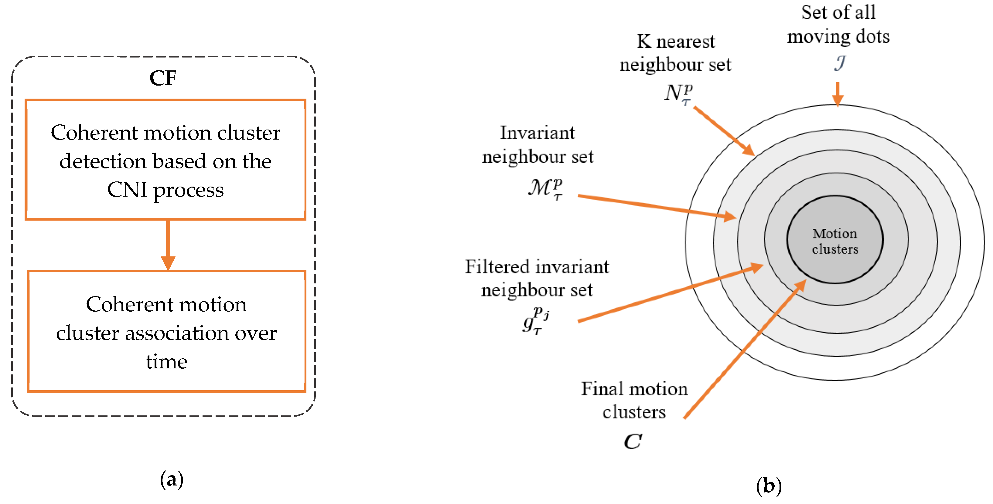
3. The Fundamental of Coherent Filtering (CF) Clustering

When feature keypoints are used to describe objects in scenes, the process of the crowd motion analysis can be converted to analyse the motion states of these keypoints. CF is proposed by Zhou et al. [36]. It is a similarity-based clustering technique, which detects the crowd’s coherent motion from crowd clutters. A general illustration of the CF process is shown in Figure 1. It functions from a microscopic-to-macroscopic consistency based on two main sequence processes that are briefly described in Section 3.1 and Section 3.2.

3.1. Coherent Motion Cluster Detection Based on Coherent Neighbor Invariance (CNI)

The coherent neighbour invariance, which is widely existing in collective scenes, can understand coherent motion detection. This section provides the details of the CNI relationship and describes its basic equations. It also provides the local neighbourhood of the moving individuals or points in terms of: (1) the invariance of spatiotemporal relationships of the points; and (2) the invariance of velocity correlations of points. The CNI process is shown in Figure 1a. It is categorized into two main sequence stages that are briefly described in Section 3.1.1 and Section 3.1.2.

3.1.1. Spatio-Temporal Invariant Points by Using Euclidian Distance Metric Stage

Initially, let the represented input moving points that contain all mixed points as $\mathcal{I}$, which are the coherent and uncoherent moving points. All the points are moving in 2-dimensional space during a period from $t$ to $t+d$, where $d$ is the time distance. Here, the points are a general term, which represents the moving points. To find the spatiotemporal invariant points, each point from the input points must be tested separately from all other points. Therefore, at time $t$, select randomly point $p$, where $p\in \mathcal{I}$ and calculate the distance between point $p$ and other point(s) $p_k$, where $p_k\in \mathcal{I}$ and $p_k\ne p$. For the calculation of the distance among the entire points, the Euclidean distance measure function is used for this purpose. It determines the quantitative degree of how close two points are. Then, find the K nearest points to point $p$ and create the K nearest neighbours (KNN) group ${{\rm N}}_t^p$ at time $t$. Accordingly, the process is performed for point$p$ to the rest of the specified period until $t+d$ to search for the KNN point set ${{\rm N}}_{\tau }^p$, where $\tau =t \to t+d$. Finally, a large graph is created to filter out points that do not satisfy the neighbourhood condition, then search for the invariant neighbour among the KNN of point $p$ from $t$ to $t+d$, and represent it as ${\mathcal{M}}_{\tau }^p$.

3.1.2. Velocity Correlated Invariant Points Stage

To identify the spatiotemporal invariant points, each point from the invariant neighbour set must be tested separately from all other points. Suppose the point $p_k$ belongs to the invariant neighbour set of point$p$, where each $p_k\in {\mathcal{M}}_{\tau }^p$. Thus, at time $t$, compute the velocity correlation between $p_k$ and $p$. Second, compute the average velocity correlation $g_{\tau }^{p_k}$ from time $t$ to $t+d$ with point $p$. Then, detect the outlier points from the invariant neighbour set ${\mathcal{M}}_{\tau }^p$ based on the $g_{\tau }^{p_k}<\lambda$ threshold, regarded as incoherent points. After thresholding, keep all the thresholds pairwise connections $(p,p_k)$in a set $\mathcal{R}$, where $p_k\in {\mathcal{M}}_{\tau }^p$. After that, build a connectivity graph from $\mathcal{R}$ to identify the coherent nodes and incoherent nodes $\mathcal{B}$ from $\mathcal{R}$ to be removed as isolated nodes. Finally, identify coherent motion clusters as $\left\{C_1,\dots ,C_J\right\}$.

3.2. Coherent Motion Cluster Association over Time

The main function of this part is to maintain the detected motion clusters $\left\{C_1,\dots ,C_J\right\}$ and associate them over time. To associate these clusters of coherent motion over time, a special variable is defined for each moving point to conserve the clustered index to the specified moving point over time. For each cluster, the cluster indices will be updated for its moving points based on the majority voting. This process keeps on updating new coherent motion clusters consistent with keeping old clusters over time.

4. Hierarchical KLT Tracklets Association (HTA) Process for Coherent Motion Detection

In this work, the Kanade–Lucas–Tomasi (KLT) feature point tracker [43,57] is utilized due to its robustness and computational efficiency [36,38,44]. The focus is on the KLT tracklets corrections for better outcomes of the subsequent tasks of the crowd clustering process.

For a specific video sequence, let $F_t$ be the tth input frame of the video $V$, where $t\in \left\{1,2, \dots , T\right\}$ and $T$ is the total frame/time number. The KLT tracker produces small trajectories (tracklets), as given in Equation (1),

$$\left\{F_t\right\}{|}_{t=1}^T \stackrel{\mathrm{KLT} \mathrm{Tracker}}{\to } \left\{t{r}_n\right\}{|}_{n=1}^N ,$$

(1)

where $t{r}_n$ is one single tracklet, tracklet number $n\in \left\{1,2,\dots ,N\right\}$, and $N$ refers to the total number of tracklets. The length of the KLT tracklets depends on several factors, as discussed in Section 1. This process produces a large pool of tracklets, $Tr=\left\{t{r}_1,\dots ,t{r}_n,\dots ,t{r}_N\right\}$, which summarizes the motion patterns observed in the scene. More formally, $t{r}_n$ can be defined as a set of points, as shown in Figure 2, which represents discrete spatial locations over time, as given in Equation (2),

$$t{r}_n \stackrel{2\mathrm{D} \mathrm{positions}}{\to } \{p_n{}_t=\left(x_{n_t},y_{n_t}\right)\}{|}_{t=t_{init }}^{t_{final}} ,$$

(2)

where $p_n{}_t\in {ℝ}^2$, it is nth tracklet’s position in $x$ and $y$ axis of the crowd at specific frame $t$. The time index $t_{init }$ and $t_{final}$ represent the lifetime of the tracklet, which is determined in period $1\le t_{init }<t_{final}\le T$. Thus, the final tracklet-position matrix $\mathbb{P}$ of the input video is defined in Equation (3),

$$\mathbb{P}=\left[\begin{array}{ccc}\begin{array}{cc}{p}_1{}_{t_{init }}& p_1{}_{t_{init+1 }}\\ p_2{}_{t_{init }}& p_2{}_{t_{init+1 }}\end{array}& \begin{array}{c}\cdots \\ \cdots \end{array}& \begin{array}{c}{p}_1{}_{t_{final}}\\ p_2{}_{t_{final}}\end{array}\\ ⋮& \ddots & ⋮\\ \begin{array}{cc}{p}_N{}_{t_{init }}& p_N{}_{t_{init+1 }}\end{array}& \cdots & p_N{}_{t_{final}}\end{array}\right]=\left[\begin{array}{c}t{r}_1\\ t{r}_2\\ ⋮\\ t{r}_N\end{array}\right].$$

(3)

The proposed HTA initialization process consists of several hierarchal steps and encompasses statistics of trajectories’ motion. This hierarchical process is shown in a block diagram with an example in Figure 3. The steps of the proposed HTA algorithm are described in detail in this section.

Table 1. Nomenclature.

Symbol	Description
$F$	Input frame
$T$	Total frames number for a given video sequence
$tr$	A single tracklet
$Tr$	Tracklets pool
$N$	Tracklets total number
$p$	One point position of a tracklet in x and y axis
$\mathbb{P}$	Tracklet-position matrix of the input video
$tre$	Tracklet that ended in ROI
$trs$	Tracklet that started in ROI
$ep$	End-point position of tre tracklet
$sp$	Start-point position of trs tracklet
$MainTr$	Tracklets vector that ended in ROI
$SubTr$	Tracklets vector that started in ROI
$O$	Tracklet orientation

illustrates the main symbols used in this paper.

4.1. Stage-1 (S1): Tracklets at Region of Interest (ROI)

Initially, it is quite essential to search for tracklets on the affected areas of the input video space that can be considered lost or disconnected tracklets. This can be done by searching for the tracklets with a missing connection. This procedure is carried out by the following steps:

Step-1:

On the video sequence $F_t$, the area in which the missing path problem will be addressed, is determined manually as the region of interest (ROI).

Step-2:

From the tracklets pool $Tr$, search for all the tracklets, which ended inside ROI, and represent it as the parent or main tracklet set, $MainTr$. Minutely, $MainT{r}_t$ are the tracklets that started before a specific time and were suddenly lost at a specific time $t$, as defined in Equation (4),

$$MainT{r}_t=\left\{tr{e}_1,\dots ,tr{e}_i,\dots ,tr{e}_I\right\},$$

(4)

where $tr{e}_i$ represents an individual tracklet that ended at ROI; $I$ is the total number of tracklets that ended inside ROI.

Step-3:

Also, search for tracklets that can be connected to the tracklets in $MainT{r}_t$. These tracklets are described as paths, which started their lifetime at ROI and are presented in another group called $SubTr$, as defined in Equation (5),

$$SubT{r}_{t+1\to t+W}=\left\{tr{s}_1,\dots ,tr{s}_j,\dots ,tr{s}_J\right\},$$

(5)

where $W$ is a temporal window stride of $t$, $J$ is the total number of tracklets that started inside ROI, and $tr{s}_j$ represents an individual tracklet, which started at any time from $t+1$ to $t+W$ in ROI.

Step-4:

Lastly, the main and sub-tracklet sets at time$t$ of this stage will be grouped, as represented in Equation (6),

$$\mathit{R}\mathit{O}{\mathit{I}}_t=\left\{MainT{r}_t,SubT{r}_{t+1\to t+W}\right\}.$$

(6)

4.2. Stage-2 (S2): Short-Path Filtering Layer (SPFL)

Some tracklets in the $\mathit{R}\mathit{O}{\mathit{I}}_t$ show unusual behaviour in the length compared to the majority of the tracklet set lengths (the tracklet’s length is the total number of its points in the tracklet’s lifetime) of $MainT{r}_t$ and $SubT{r}_{t+1\to t+W}$. These small paths produce wrong results and affect the process of associating the successions to the correct paths. Therefore, this short-path filter layer (SPFL) seeks to detect the outlier tracklets by some steps as follows:

Step-1:

Calculate the lengths of all collected tracklets from Stage-1 and get the average as given in Equation (7),

$$AvgL=\frac{1}{2}\left(\frac{1}{I}{\displaystyle \sum }_{i=1}^{I}length\left(tr{e}_i\right)+\frac{1}{J}{\displaystyle \sum }_{j=1}^{J}length\left(tr{s}_j\right)\right),$$

(7)

where $I$ and $J$ are the total tracklet number for $MainT{r}_t$ and $SubT{r}_{t+1\to t+W}$, respectively. Finding the average result provides information about the lengths of the normal paths. This value is useful in filtering very short lengths, as can be seen in the next step.

Step-2:

Keep the tracklets that can be considered candidate tracklets based on an average threshold $t{h}_{avg}=AvgL/\epsilon$, where the value of $\epsilon$ is an empirical value, which varies from video to video. For example, to remove the short-path tracklets from the $MainT{r}_t$ set, Equation (8) is considered,

$$SPFL\_Con\left(MainT{r}_t\right)=\left\{\begin{array}{c}\mathrm{Keep} \mathrm{as} tr{e}_l^{spfl} ,length\left(tr{e}_i\right) \ge t{h}_{avg} \\ \mathrm{Ignore} \left(tr{e}_i\right) , \mathrm{otherwise} \end{array}\right.,$$

(8)

where $SPFL\_Con$ represents the tracklets length consistency. This filtering process is applied to $MainT{r}_t$ and $SubT{r}_{t+1\to t+W}$ to remove all the short paths in both sets.

Step-3:

As a result, the updated tracklets sets after filtering the short paths will be considered in Equation (9),

$$\begin{array}{ll}Match\_T{r}_t& =\left\{MainT{r}_t^{spfl},SubT{r}_{t+1\to t+W}^{spfl}\right\}\\ & =\left\{\left(tr{e}_1^{spfl},\dots ,tr{e}_l^{spfl},\dots ,tr{e}_L^{spfl}\right),\left(tr{s}_1^{spfl},\dots , tr{s}_k^{spfl},\dots ,tr{s}_K^{spfl}\right)\right\},\end{array}$$

(9)

where L is the total tracklet number of $MainT{r}_t$ and K is the total tracklet number of $SubT{r}_{t+1\to t+W}$.

4.3. Stage-3 (S3): Position Filtering Layer (PFL)

After applying the SPFL layer, it is important to find tracklets from $SubT{r}_{t+1\to t+W}^{spfl}$, which are near the tracklets of $MainT{r}_t^{spfl}$ and have the potential to be associated with a single path in terms of neighbourhoods. Starting from this stage until the end of this algorithm, the process will be applied to one selected individual tracklet $tr{e}_l^{spfl}$ from $MainT{r}_t^{spfl}$ to find the most adjacent tracklets from $SubT{r}_{t+1\to t+W}^{spfl}$ set, which can be done in the following steps:

Step-1:

For an individual tracklet $tr{e}_l^{spfl}$ at time $t$, find its end-point position in $x$ and $y$ from the tracklet-position matrix, as given in Equation (10),

$$e{p}_l=p_{l_{t_{final}}}^{spfl} .$$

(10)

Step-2:

Find the start-point positions of the entire candidate tracklets from $SubT{r}_{t+1\to t+W}^{spfl}$, as given in Equation (11),

$$\left(s{p}_1,\dots ,s{p}_k,\dots ,s{p}_K\right)=\left(p_{1_{t_{init }}}^{spfl},\dots ,p_{k_{t_{init }}}^{spfl},\dots ,p_{K_{t_{init }}}^{spfl}\right).$$

(11)

Step-3:

Calculate the position coordinates Euclidian distance of the endpoint $e{p}_l$ with all the start points of the sub-tracklets, as given in Equation (12),

$$Ec{d}_{lk}\left(e{p}_l,s{p}_k\right)=\sqrt{{\left|e{p}_l-s{p}_k\right|}^2}=\sqrt{{\left(x_l-x_k\right)}^2+{\left(y_l-y_k\right)}^2}.$$

(12)

Step-4:

Apply the position consistency to filter out tracklets that do not satisfy the neighbouring condition, as given in Equation (13),

$$PFL\_Con\left(tr{e}_l^{spfl},SubT{r}_{t+1\to t+W}^{spfl}\right)=\left\{\begin{array}{c}\mathrm{Keep} \mathrm{as} tr{s}_m^{pfl} ,Ec{d}_{lk}\le t{h}_{pos}\\ \mathrm{Ignore} tr{s}_k^{spfl} , \mathrm{otherwise} \end{array}\right.,$$

(13)

where $m\in \left\{1,2, \dots , M\right\}$ and $M$ represent the tracklet’s total number of updated $SubT{r}_{t+1\to t+W}^{pfl}$ set. The $t{h}_{pos}$ represents the neighbourhood threshold; it is an empirical value that varies from video to video.

Step-5:

The updated tracklet set in this step is represented as the end, as given in Equation (14),

$$Match\_t{r}_t=\left\{tr{e}_l^{spfl},\left(SubT{r}_{t+1\to t+W}^{pfl}\right)\right\}.$$

(14)

4.4. Stage-4 (S4): Orientation Filtering Layer (OFL)

After identifying the matching tracklets using the PFL stage, the next step is to ensure that the orientations of the tracklets are uniform. In this layer, the tracklet orientations are calculated for both the main and sub-tracklets.

Step-1:

The orientation of an individual main tracklet $tr{e}_l^{spfl}$ at time $t$ is calculated by considering the directions of its position points in a frame distance, as given in Equation (15),

$$O_l=\frac{1}{FrDist}{\displaystyle \sum }_{k=t-FrDist+1}^{t}atan2\left(y_{l_k}-y_{l_{k-1}},x_{l_k}-x_{l_{k-1}}\right) 180°/\pi ,$$

(15)

where $FrDist$ is a frame distance that $0$$<FrDist\le W$ and $0°\le O_i\le 360°$.

Step-2:

Likewise, if the sub-tracklet $tr{s}_m^{pfl}$ is assumed to start from time $t+1$, then its orientation can be calculated, as given in Equation (16),

$$O_m=\frac{1}{FrDist}{\displaystyle \sum }_{k=t+1}^{\left(t+1\right)+FrDist}atan2\left(y_{m_{k+1}}-y_{m_k},x_{m_{k+1}}-x_{m_k}\right) 180°/\pi ,$$

(16)

where $0°\le O_m\le 360°$.

Step-3:

Apply the orientation consistency to filter out sub-tracklets that do not satisfy the orientation condition with the main tracklet $tr{e}_i^{spfl}$, as given in Equation (17),

$$OFL\_Con\left(tr{e}_l^{spfl},\left(SubT{r}_{t+1\to t+W}^{pfl}\right)\right)=\left\{\begin{array}{c}\mathrm{Keep} \mathrm{as} tr{s}_q^{ofl} ,||O_l-O_m|| \le t{h}_{ori} \\ \mathrm{Ignore} tr{s}_m^{pfl} , \mathrm{otherwise} \end{array}\right.,$$

(17)

where $q\in \left\{1,2, \dots , Q\right\}$ and $Q$ represents the total number of updated $SubT{r}_{t+1\to t+W}^{ofl}$ set and $t{h}_{ori}$ represents the orientation threshold; it is an empirical value that varies from video to video.

Step-4:

The updated match tracklets set in this layer will be finally grouped, as given in Equation (18),

$$Match\_t{r}_t=\left\{tr{e}_l^{spfl},\left(SubT{r}_{t+1\to t+W}^{ofl}\right)\right\}.$$

(18)

4.5. Stage-5 (S5): Correlation Filtering Layer (CFL)

The previous filtering layers tried to search for the best candidate tracklets to connect the main and sub-tracklets as one hale path, depending on their lengths, positions, and orientations of tracklet points. These steps can ensure the selection of the best pair of tracklets, which achieves the best homogeneity among their natural behaviour movements. In the case of obtaining more than one candidate tracklet after successfully passing all these filtering layers, it is necessary to study these tracklet points at the image pixel level through the use of correlation coefficient statistics to ensure that the best path is chosen as the final result.

More specifically, the correlation coefficient measure [58,59], (also known as Pearson’s correlation coefficient) is a method, which is used to establish the degree of probability that a linear relationship exists between two measured quantities or variables. A single quantity represents the matrix values of 2D image pixels for one tracklet point. The suggested idea in this layer is to compare the endpoint value of the main tracklet $tr{e}_l^{spfl}$with the starting point value of the candidate sub-tracklet $tr{s}_q^{ofl}$. The following steps explain the process in detail:

Step-1:

At time $t$, find the position of the endpoint $e{p}_l$ of the tracklet $tr{e}_l^{spfl}$ in the image plane. Then, calculate its intensity pixel values matrix $A_l{}_{ab}$, where $a$ and $b$ represent the size of adjacent pixels window.

Step-2:

From time $t+1$ to $t+W$, find the position of the start point $s{p}_q$ of a sub-tracklet set. For example, the intensity pixel value of the endpoint of $tr{s}_q^{ofl}$ in the image, the plane is represented as $B_q{}_{ab}$.

Step-3:

Measure the pixel correlation coefficient $Co{r}_{lq}$ among positions $e{p}_l$ and $s{p}_q$, as given in Equation (19),

$$Co{r}_{lq}=\frac{{{\displaystyle \sum }}_a{{\displaystyle \sum }}_b\left(A_l{}_{ab}-\overline{A_l}\right)\times \left( B_q{}_{ab}-\overline{ B_q}\right)}{\sqrt{({{\displaystyle \sum }}_a{{\displaystyle \sum }}_b{\left(A_l{}_{ab}-\overline{A_l}\right)}^2)\times ({{\displaystyle \sum }}_a{{\displaystyle \sum }}_b{\left( B_q{}_{ab}-\overline{ B_q}\right)}^2) }} ,$$

(19)

where $\overline{A_l}$ and $\overline{ B_q}$ are the mean of $A_l{}_{ab}$ and $B_q{}_{ab}$, respectively. The correlation coefficient ranges from $-1$ for perfect negatively correlated results, through $0$ when there is no correlation, to $1$ when the results are identical.

Step-4:

Then, apply correlation consistency to filter out all sub-tracklets that do not satisfy the correlation condition with the main tracklet, as given in Equation (20),

$$CFL\_Con\left(tr{e}_l^{spfl},SubT{r}_{t+1\to t+W}^{ofl}\right)=\left\{\begin{array}{c}\mathrm{Keep} \mathrm{as} tr{s}_r^{cfl} , Co{r}_{lq} \le t{h}_{cor} \\ \mathrm{Ignore} tr{s}_q^{ofl} , \mathrm{otherwise} \end{array}\right.,$$

(20)

where $r\in \left\{1,2, \dots , R\right\}$ and $R$ represent the total number of updated $SubT{r}_{t+1\to t+W}^{cfl}$ set and $t{h}_{cor}$ represents the correlation threshold, which is an empirical value that varies from video to video. Lastly, the updated match tracklets set in this step are given in Equation (21),

$$Match\_t{r}_t=\left\{tr{e}_l^{spfl},\left(SubT{r}_{t+1\to t+W}^{cfl}\right)\right\} .$$

(21)

Step-5:

The final match sub-tracklets from Equation (21) are ranked in ascending order as $\uparrow Match\_t{r}_t$ from the closest correlation related to the least correlation related.

Step-6:

Then, the first sub-tracklet in $\uparrow Match\_t{r}_t$ will be the best candidate to be connected with $tr{e}_l^{spfl}$ as one big path, as given in Equation (22),

$$t{r}_l^{new} :tr{e}_l^{spfl} \stackrel{Connect}{\leftrightarrow } tr{s}_r^{cfl},$$

(22)

where $t{r}_l^{new}$ is the new tracklet after connecting $tr{e}_l^{spfl}$ and $tr{s}_r^{cfl}$.

Step-7:

Update $t{r}_i^{new}$ to the enhanced KLT tracklets’ set.

Figure 4 demonstrates a spatiotemporal schematic example of applying the HTA algorithm, which shows a connection between two separated tracklets. Tracklets $tr{e}_1$ and $tr{s}_3$ are a single entity path after fulfilling the required conditions of the HTA process. At the end of this section, all raw KLT tracklets are supposed to be updated by the HTA algorithm as new enhanced KLT tracklets. This enhanced KLT feature will be fed as input data to the CF for coherent motion detection.

Finally, the proposed HTA framework is summarized in Algorithm 1. It consists of five stages, including ROI, SPFL, PFL, OFL, and CFL. All the stages have an overall complexity of cost estimation as O(N²), where N is the number of tracking points.

Algorithm 1: The proposed HTA algorithm.

Input: Video clip frames F.

Output: Coherent motion cluster $\left\{C_t^j\right\}$

5. Evaluation Metrics

Evaluation analysis is a fundamental part of the clustering process because it indicates the quality of the clustering results. It reveals to what extent these results are good if compared to other clustering results produced by other algorithms. There are different criteria to assess the goodness of the output clusters. It is worth mentioning that these evaluation metrics are used alternatively based on the purpose of the designed framework. In this study, Purity, Normalized Mutual Information Index (NMI), Rand Index (RI), and F-measure (Fm) were used to evaluate the clustering outcomes. This section provides an overview of these evaluation metrics.

Purity is an external evaluation criterion of cluster quality. It determines the dominant labels in each cluster and describes the extent to which groups match the references [60]. Usually, good clustering solutions have high-purity values. Purity is estimated by using Equation (23),

$$purity\left(\mathsf{\Omega },ℂ\right)=\frac{1}{N}{\displaystyle \sum }_k\underset{j}{\max }\left|{\omega }_k\cap c_j\right| ,$$

(23)

where $N$ is the number of observations (data points), $\mathsf{\Omega }=\left\{{\omega }_1,{\omega }_2,\dots ,{\omega }_k\right\}$ is the set of clusters, and $ℂ=\left\{c_1,c_2,\dots ,c_j\right\}$ are the corresponding ground truth classes.

Rand index (RI) [61] is a clustering evaluation metric, which measures the similarity between two clusters (i.e., partitions) by considering how each pair of data points is assigned in each clustering. It equals the number of motion pairs that are either placed in an entity or assigned to separate entities in both $ℂ$ and $\mathsf{\Omega }$, normalized by the total number of mentioned pairs in each partition [62]. RI is obtained by using Equation (24) as follows,

$$RI\left(\mathsf{\Omega },ℂ\right)=\frac{TP+TN}{TP+FP+FN+TN} ,$$

(24)

where a true positive (TP) decision assigns two points (pair of points) to the same cluster if and only if they are similar. A true negative (TN) decision assigns two dissimilar points to different clusters. The two types of errors are: a false positive (FP) decision assigns two dissimilar points to the same cluster; and a false negative (FN) decision assigns two similar points to different clusters.

Normalized Mutual Information (NMI) index [63] measures the information that $\mathsf{\Omega }$ and $ℂ$ share. NMI is based on the shared object membership with a scaling factor that corresponds to the number of objects in the respective clusters. Formally, it is obtained by using Equation (25),

$$NMI\left(\mathsf{\Omega },ℂ\right)=\frac{I\left(\mathsf{\Omega };ℂ\right)}{\left[H\left(\mathsf{\Omega }\right)+H\left(ℂ\right)\right]/2}.$$

(25)

$I\left(\mathsf{\Omega };ℂ\right)$ is the mutual information [64] between cluster and class labels. $H\left(\mathsf{\Omega }\right)$ and $H\left(ℂ\right)$ are the entropy of the cluster and class labels, respectively.

$$I\left(\mathsf{\Omega };ℂ\right)=H\left(\mathsf{\Omega }\right)-H\left(\mathsf{\Omega }|ℂ\right),$$

(26)

$$H\left(\mathsf{\Omega }\right)=-{\displaystyle \sum }_{k}P\left({\omega }_k\right)log\left({\omega }_k\right),$$

(27)

$$H\left(ℂ\right)=-{\displaystyle \sum }_{j}P\left(c_j\right)log\left(c_j\right),$$

(28)

where $P\left({\omega }_k\right)$ and $P\left(c_j\right)$ are the probabilities of a document being in a cluster ${\omega }_k$ and class $c_j$. $I\left(\mathsf{\Omega };ℂ\right)$ in Equation (26) measures the amount of information by which our knowledge about the classes increases [65].

F-measure (Fm) [66] measures the accuracy using two statistics, namely precision P and recall R. P is the ratio of true positive TP to all predicted TP + FP, as given in Equation (29). The recall is the ratio of TP to all predicted TP + FN, as given in Equation (30),

$$P\left(\mathsf{\Omega },ℂ\right)=\frac{TP}{TP+FP},$$

(29)

$$R\left(\mathsf{\Omega },ℂ\right)=\frac{TP}{TP+FN}.$$

(30)

TP refers to the positive data points that are accurately labelled by the algorithm. FP denotes the negative data points that are incorrectly labelled as positives. Finally, the positive data point, which is mislabelled as negative, is referred to as FP [66]. F-measure is obtained by using Equation (31),

$$Fm\left(\mathsf{\Omega },ℂ\right)=\frac{2PR}{P+R} .$$

(31)

6. Experimental Results

The purpose of the proposed HTA framework is to address the disconnected tracklets problem of the input KLT features and set appropriate fixing among them to enhance the performance of motion crowd clustering. In other words, HTA can be described as an enhanced initialization strategy for trajectories before crowd detection. To validate the effectiveness of the HTA algorithm, Coherent Filtering (CF) [36] is adopted to apply and compare the collective motion detection on two different input KLT features. The input features are: (1) raw KLT tracklets; and (2) enhanced KLT tracklets. The raw KLT tracklets are the input features, which are extracted from the CUHK crowd dataset [67]. The enhanced KLT tracklets are the tracklets, which are produced by the proposed HTA algorithm on the raw KLT features. Hence, the proposed HTA framework has been tested on video clips from the CUHK crowd dataset. The performance of the motion crowd clustering is evaluated by using qualitative and quantitative analysis methods, including Purity, NMI, RI, and F-measure evaluation metrics. The parameter settings, which were used for the HTA algorithm, are summarized in

Table 2. Experimental parameter settings for the HTA algorithm.

Parameter	Discerption	Value
$t{h}_{avg}$	Average threshold	$t{h}_{avg}=AvgL/\epsilon$$, \mathrm{where} \epsilon =0.5$
$t{h}_{pos}$	Position threshold	5
$t{h}_{ori}$	Orientation threshold	$30°$
$t{h}_{cor}$	Correlation threshold	0.5
$FrDist$	Time/frame distance	5
$W$	Temporal window stride	5

.

The FrDist and W represent a short period of frame distance processing and set as used in [36]. Threshold parameters $\epsilon$, $t{h}_{pos}$, $t{h}_{ori}$, and $t{h}_{cor}$ are adjusted by taking their average value according to the experiments, which were carried out on the CUHK crowd dataset.

6.1. CUHK Crowd Dataset

The HTA framework has been tested on the CUHK crowd dataset [67]. It is a collection of real videos with their raw KLT tracklets and ground truth. It includes crowd videos with various densities, directions, and perspective scales, obtained from many different environments, e.g., shopping malls, airports, streets, and public parks. Figure 5 shows some samples of the frame scene and its KLT keypoints ground truth from the CUHK crowd dataset. It consists of 474 video clips from 215 scenes. Some of these clips were captured by the authors (55 clips) and the rest were collected from Pond5 and Getty Image. The resolutions of the video clips varied, mutating from 480 × 360 to 1920 × 1080. The frame rates are different as well, varying from 20 to 30 frames per second. It is worth noting that only 300 video clips have their complete data (which are the video clip, the raw KLT tracklet features, and the ground truth). The rest of the 174 video clips do not have their ground truth and, therefore, cannot be used for quantitative evaluation.

6.2. Disconnected Trajectories on Raw KLT Features

The HTA algorithm has been applied to the raw KLT tracklets of all 300 video clips in the CUHK crowd dataset. Although the weak KLT tracklets have been previously filtered and smoothed by the authors in CUHK, (2014), there are still many video clips that have broken and disconnected KLT tracklets. As discussed in Section 1, this is due to a glitch in the KLT features, which may occur due to some factors, such as frame rate, camera position, and intensity of motion. However, not all 300 video clips contain broken trajectories. Several clips completed smooth tracklets without any destruction. This indicates that the performance of the proposed HTA algorithm depends on the amount of the discontinuous tracklets in each video clip, which will be further investigated in the experimental results in Section 6.3 and Section 6.4.

To illustrate the idea and put it into perspective, Figure 6 shows some selected examples from the CUHK crowd datasets that have different discontinuous tracklets. For example, video clip number 32 in the first line contains a total of 987 raw KLT tracklets, presented in blue color in its plot. All those tracklets are stable and complete during their lifetime and free of any broken trajectories. This is due to the nature of the scene, where the crowd (the walking soldiers) are moving steadily in one direction. The other two examples, i.e., video clips (No. 81 and No. 115) have a total number of raw KLT tracklets of 2091 and 1087, respectively. It is noticeable that the moving pedestrians in these two video clips are moving in parallel with some different directions, which can, in turn, generate some disconnected tracklets. The plots in Figure 6b show the presence of the broken tracklets in red dots. The disconnected KLT tracklets are calculated in percentage with values of 10.8% and 2.1% for both video clips (No. 81 and No. 115), respectively.

Based on the examination, which was carried out on 300 video clips of the CUHK dataset, it was found that the presence of disconnected tracklets ranged from 0 to 11%, as shown in Figure 7. The next sections discuss the impact of disconnected tracklets on the performance of crowd clustering and detection.

6.3. Qualitative Result Discussion of Motion Crowd Clustering Using HTA

In this section, two video clip examples from the CUHK crowd dataset were selected for illustrative purposes. These video clips have a high percentage of disconnected KLT tracklets in their input raw data. These examples show the effectiveness of the proposed HTA framework regarding the quality of crowd clustering, as shown in Figure 8 and Figure 9.

The example in Figure 8 shows a common case that affects the KLT trajectories’ consistency, which is the presence of some objects in front of the camera, partially hiding the moving pedestrians, such as the presence of branches of some trees, as observed in the image. This situation leads to the separation of several trajectories into small parts during the lifetime of the scene. Figure 8a exhibits a sample scene of video clip No. 16, which contains a 109-frame image sequence of 20 frames per second. Based on the input data test of video clip No. 16, the raw KLT tracklets have some broken trajectories. The percentage of broken tracklets is calculated as 7.41% of the total input raw KLT tracklets of video clip No. 16. Thus, this calculated ratio is the target tracklets of the HTA algorithm used to enhance the input KLT features. The scene in Figure 8b shows the ground truth of the tracklets at frame 45 provided by the CUHK crowd dataset. Figure 8c,d show the visual performance of crowd clustering by applying CF on raw and enhanced KLT tracklets, respectively. As observed in Figure 8c, in the example by the red boxes, the moving KLT points, which were generated by the CF using the input raw data, are separated into small colored clusters. This is due to the presence of many disconnected tracklets that led to the separation of the trajectories from the main cluster. On the other hand, in Figure 8d, the level of clustering showed further improvement due to the connection of the broken trajectories. This connection made the resultant clusters last longer without splitting over time, as clarified in the example by the orange box. The enhanced KLT tracklets performed better in terms of motion clustering consistency.

The same situation occurred with the video clip No. 81, example in Figure 9. It has some problems in the frame rate progressing, creating almost 10.83% of candidate broken tracklets for the re-connection process. Figure 9a exhibits a sample scene of the video clip that contains a 208-frame image sequence; 20 frames per second. The scene in Figure 9b shows the ground truth of the tracklets in frame 50. Figure 9c,d show the visual performance of crowd clustering by applying CF on raw and enhanced KLT tracklets, respectively. The enhanced KLT tracklets performed better in terms of the motion clustering quality.

6.4. Quantitative Result Discussion of Motion Crowd Clustering Using HTA

In this section, the performance analysis of motion crowd clustering using the HTA algorithm is evaluated on the CUHK crowd data. The metrics, which were used for evaluation in these experiments, are Purity, NMI, RI, and F-measure. The experimental average results on the whole dataset are divided into three categories based on the percentage degree of candidate KLT tracklets’ presence, as reported in

Table 3. Average experimental results (for 300 video clips) with Purity, NMI, RI, and Fm on the CUHK crowd dataset.

Index	Video Clips with a Percentage of Disconnected Tracklets	CF on Raw KLT				CF on Enhanced KLT
		Purity	NMI	RI	Fm	Purity	NMI	RI	Fm
1	68 video clips with (≥6%)	0.85	0.44	0.79	0.81	0.89	0.47	0.82	0.84
2	91 video clips with (≥3% & <6%)	0.84	0.44	0.76	0.77	0.87	0.48	0.79	0.79
3	141 video clips with (<3%)	0.86	0.51	0.79	0.82	0.86	0.51	0.79	0.82

and Figure 10.

The experimental results of index 1 were carried out on a total of 68 video clips that have candidate KLT tracklets to be connected within the range, equal to or higher than 6%. The enhanced KLT tracklets by using the HTA algorithm outperformed the raw KLT tracklets in terms of coherent motion clustering with these average values: Purity = 0.89, NMI = 0.47, RI = 0.82, and F-measure = 0.84. The experimental results of index 2 were carried out on 91 video clips that have candidate KLT tracklets to be connected within the range of less than 6% and greater or equal to 3%. An improvement was found with the following average results values: Purity = 0.87, NMI = 0.48, RI = 0.79, and F-measure = 0.79. The experimental results of index 3 were carried out on a total of 141 video clips that have candidate KLT tracklets to be connected in less than 3%. However, no significant progress was found in the overall average. This is because the disconnected tracklets had no effect, and they were not broadly present during the clip’s lifetime.

Although the CUHK crowd dataset contains video clips with smoothed KLT tracklets, there is a percentage of the tracklets that can be considered broken tracklets. By understanding the results presented previously, it is obvious that this improvement shows the efficiency when the number of disconnected tracklets is large enough. This is clear from bar graphs in Figure 10, index 1, and index 2 compared to index 3. It is also worth mentioning that the CUHK crowd data does not contain the full ground truth for all video frames. For each video clip, there is only one frame available with its ground truth for evaluation. This does not provide an adequate result for the evaluation; therefore, it is considered one of the shortcomings of the data in terms of assessment.

To recap, it can be concluded that the enhanced KLT tracklet features, which were improved by the proposed HTA algorithm, have significantly improved the efficiency of crowd clustering in contrast to using the raw KLT tracklets features in terms of Purity, NMI, RI, and F-measure of the obtained clustering solutions. This improvement underscores efficiency when the number of disconnected tracklets is large enough. The case of the ratio of the disconnected tracklets, which is more than 3%, is considered in this study.

7. Conclusions

In this paper, the effect of disconnected tracklets on coherent motion filtering (CF) is investigated from the visual point of view. The disconnected tracklets can have a significant impact on collective motion detection. Based on the CNI behaviour study, a rich set of tracklets properties were designed, including trajectory positions, paths, orientations, and pixel correlations. A robust hierarchical tracklet association algorithm is proposed to improve the input KLT features for CF. The algorithm allows searching for broken KLT tracklets that are usually found in video clips. This reduces the negative impact of this disconnection by associating them using the hierarchy association process, which gives tracklets a longer life in the video clip. The experimental results showed that the enhanced KLT tracklet features by applying the proposed HTA algorithm have significantly improved the efficiency of crowd clustering in contrast to using the raw KLT tracklets only as the input features in terms of Purity, NMI, RI, and F-measure.

For future work, based on examining the working mechanism of the proposed HTA framework, it is noticeable that this framework requires some parameters to be known in advance, such as $\epsilon$, $t{h}_{pos}$, $t{h}_{ori}$, and $t{h}_{cor}$. These parameters depend on the nature of the video clip. Hence, one of the ideas to improve the current research work is to tune these parameters automatically without prior knowledge. This can be done by extracting some characteristics from each video clip that describe the nature of the crowd in the video. This addition can provide the capability for the proposed algorithm framework to become fully unsupervised and more truly intelligent while solving real-world problems. In addition, the proposed algorithm is designed based on studying the CNI concepts, thereby making it operate better in the CF algorithm. However, a generalized HTA algorithm is required to be designed considering most of the similarity-based clustering methods.

References

1. Chaudhary, D.; Kumar, S.; Dhaka, V.S. Video Based Human Crowd Analysis Using Machine Learning: A Survey. Comput. Methods Biomech. Biomed. Eng. Imaging Vis. 2022, 10, 113–131. [Google Scholar] [CrossRef]
2. Muhammed, D.A.; Rashid, T.A.; Alsadoon, A.; Bacanin, N.; Fattah, P.; Mohammadi, M.; Banerjee, I. An Improved Simulation Model for Pedestrian Crowd Evacuation. Mathematics 2020, 8, 2171. [Google Scholar] [CrossRef]
3. Martín-Santamaría, R.; López-Sánchez, A.D.; Delgado-Jalón, M.L.; Colmenar, J.M. An Efficient Algorithm for Crowd Logistics Optimization. Mathematics 2021, 9, 509. [Google Scholar] [CrossRef]
4. Bendali-Braham, M.; Weber, J.; Forestier, G.; Idoumghar, L.; Muller, P.-A. Recent Trends in Crowd Analysis: A Review. Mach. Learn. Appl. 2021, 4, 100023. [Google Scholar] [CrossRef]
5. Yang, G.; Zhu, D. Survey on Algorithms of People Counting in Dense Crowd and Crowd Density Estimation. Multimed. Tools Appl. 2022. [Google Scholar] [CrossRef]
6. Fan, Z.; Zhang, H.; Zhang, Z.; Lu, G.; Zhang, Y.; Wang, Y. A Survey of Crowd Counting and Density Estimation Based on Convolutional Neural Network. Neurocomputing 2022, 472, 224–251. [Google Scholar] [CrossRef]
7. Zhong, M.; Tan, Y.; Li, J.; Zhang, H.; Yu, S. Cattle Number Estimation on Smart Pasture Based on Multi-Scale Information Fusion. Mathematics 2022, 10, 3856. [Google Scholar] [CrossRef]
8. Saleh, S.A.M.; Suandi, S.A.; Ibrahim, H. Recent Survey on Crowd Density Estimation and Counting for Visual Surveillance. Eng. Appl. Artif. Intell. 2015, 41, 103–114. [Google Scholar] [CrossRef]
9. Wei, X.; Liu, J.-C.; Bi, S. Uncertainty Quantification and Propagation of Crowd Behaviour Effects on Pedestrian-Induced Vibrations of Footbridges. Mech. Syst. Signal Process. 2022, 167, 108557. [Google Scholar] [CrossRef]
10. Yu, Y.; Shen, W.; Huang, H.; Zhang, Z. Abnormal Event Detection in Crowded Scenes Using Two Sparse Dictionaries with Saliency. J Electron. Imaging 2017, 26, 33013. [Google Scholar] [CrossRef]
11. Yi, S.; Li, H.; Wang, X. Understanding Pedestrian Behaviors from Stationary Crowd Groups. In Proceedings of the IEEE Conference on Computer Vision and Pattern Recognition, Boston, MA, USA, 7–15 June 2015; pp. 3488–3496. [Google Scholar]
12. Fradi, H.; Luvison, B.; Pham, Q.C. Crowd Behavior Analysis Using Local Mid-Level Visual Descriptors. IEEE Trans. Circuits Syst. Video Technol. 2016, 27, 589–602. [Google Scholar] [CrossRef]
13. Al-Sa’d, M.; Kiranyaz, S.; Ahmad, I.; Sundell, C.; Vakkuri, M.; Gabbouj, M. A Social Distance Estimation and Crowd Monitoring System for Surveillance Cameras. Sensors 2022, 22, 418. [Google Scholar] [CrossRef]
14. Pai, A.K.; Chandrahasan, P.; Raghavendra, U.; Karunakar, A.K. Motion Pattern-Based Crowd Scene Classification Using Histogram of Angular Deviations of Trajectories. Vis. Comput. 2022, 39, 557–567. [Google Scholar] [CrossRef]
15. Wang, X.; Zheng, S.; Yang, R.; Zheng, A.; Chen, Z.; Tang, J.; Luo, B. Pedestrian Attribute Recognition: A Survey. Pattern Recognit. 2022, 121, 108220. [Google Scholar] [CrossRef]
16. Sindagi, V.A.; Patel, V.M. A Survey of Recent Advances in Cnn-Based Single Image Crowd Counting and Density Estimation. Pattern Recognit. Lett. 2018, 107, 3–16. [Google Scholar] [CrossRef] [Green Version]
17. Shao, J.; Loy, C.C.; Kang, K.; Wang, X. Crowded Scene Understanding by Deeply Learned Volumetric Slices. IEEE Trans. Circuits Syst. Video Technol. 2016, 27, 613–623. [Google Scholar] [CrossRef]
18. Lohithashva, B.H.; Aradhya, V.N.M. Violent Video Event Detection: A Local Optimal Oriented Pattern Based Approach. In Proceedings of the International Conference on Applied Intelligence and Informatics, Nottingham, UK, 30 July 2021; pp. 268–280. [Google Scholar]
19. Yu, J.; Lee, Y.; Yow, K.C.; Jeon, M.; Pedrycz, W. Abnormal Event Detection and Localization via Adversarial Event Prediction. IEEE Trans. Neural Netw. Learn. Syst. 2022, 33, 3572–3586. [Google Scholar] [CrossRef]
20. Jebur, S.A.; Hussein, K.A.; Hoomod, H.K.; Alzubaidi, L.; Santamaría, J. Review on Deep Learning Approaches for Anomaly Event Detection in Video Surveillance. Electronics 2023, 12, 29. [Google Scholar] [CrossRef]
21. Wang, J.; Xu, Z. Spatio-Temporal Texture Modelling for Real-Time Crowd Anomaly Detection. Comput. Vis. Image Underst. 2016, 144, 177–187. [Google Scholar] [CrossRef]
22. Zhou, T.; Zheng, L.; Peng, Y.; Jiang, R. A Survey of Research on Crowd Abnormal Behavior Detection Algorithm Based on YOLO Network. In Proceedings of the 2022 2nd International Conference on Consumer Electronics and Computer Engineering (ICCECE), Guangzhou, China, 14–16 January 2022; pp. 783–786. [Google Scholar]
23. Lalit, R.; Purwar, R.K. Crowd Abnormality Detection Using Optical Flow and GLCM-Based Texture Features. J. Inf. Technol. Res. (JITR) 2022, 15, 1–15. [Google Scholar] [CrossRef]
24. Ekanayake, E.M.C.L.; Lei, Y.; Li, C. Crowd Density Level Estimation and Anomaly Detection Using Multicolumn Multistage Bilinear Convolution Attention Network (MCMS-BCNN-Attention). Appl. Sci. 2023, 13, 248. [Google Scholar] [CrossRef]
25. Benabbas, Y.; Ihaddadene, N.; Djeraba, C. Motion Pattern Extraction and Event Detection for Automatic Visual Surveillance. EURASIP J. Image Video Process. 2010, 2011, 163682. [Google Scholar] [CrossRef] [Green Version]
26. Han, T.; Yao, H.; Sun, X.; Zhao, S.; Zhang, Y. Unsupervised Discovery of Crowd Activities by Saliency-Based Clustering. Neurocomputing 2016, 171, 347–361. [Google Scholar] [CrossRef]
27. Solmaz, B.; Moore, B.E.; Shah, M. Identifying Behaviors in Crowd Scenes Using Stability Analysis for Dynamical Systems. IEEE Trans. Pattern Anal. Mach. Intell. 2012, 34, 2064–2070. [Google Scholar] [CrossRef] [PubMed]
28. Zhou, B.; Tang, X.; Wang, X. Learning Collective Crowd Behaviors with Dynamic Pedestrian-Agents. Int. J. Comput. Vis. 2015, 111, 50–68. [Google Scholar] [CrossRef] [Green Version]
29. Li, T.; Chang, H.; Wang, M.; Ni, B.; Hong, R.; Yan, S. Crowded Scene Analysis: A Survey. IEEE Trans. Circuits Syst. Video Technol. 2014, 25, 367–386. [Google Scholar] [CrossRef] [Green Version]
30. Ali, S.; Shah, M. A Lagrangian Particle Dynamics Approach for Crowd Flow Segmentation and Stability Analysis. In Proceedings of the 2007 IEEE Conference on Computer Vision and Pattern Recognition, Minneapolis, MN, USA, 17–22 June 2007; pp. 1–6. [Google Scholar]
31. Mehran, R.; Moore, B.E.; Shah, M. A Streakline Representation of Flow in Crowded Scenes. In Proceedings of the European Conference on Computer Vision, Crete, Greece, 5–11 September 2010; pp. 439–452. [Google Scholar]
32. Wu, S.; San Wong, H. Crowd Motion Partitioning in a Scattered Motion Field. IEEE Trans. Syst. Man Cybern. Part B Cybern. 2012, 42, 1443–1454. [Google Scholar]
33. Song, L.; Jiang, F.; Shi, Z.; Katsaggelos, A.K. Understanding Dynamic Scenes by Hierarchical Motion Pattern Mining. In Proceedings of the 2011 IEEE International Conference on Multimedia and Expo, Barcelona, Spain, 11–15 July 2011; pp. 1–6. [Google Scholar]
34. Zhou, B.; Wang, X.; Tang, X. Random Field Topic Model for Semantic Region Analysis in Crowded Scenes from Tracklets. In Proceedings of the CVPR 2011, Colorado Springs, CO, USA, 20–25 June 2011; pp. 3441–3448. [Google Scholar]
35. Fu, W.; Wang, J.; Li, Z.; Lu, H.; Ma, S. Learning Semantic Motion Patterns for Dynamic Scenes by Improved Sparse Topical Coding. In Proceedings of the 2012 IEEE International Conference on Multimedia and Expo, Melbourne, VIC, Australia, 9–13 July 2012; pp. 296–301. [Google Scholar]
36. Zhou, B.; Tang, X.; Wang, X. Coherent Filtering: Detecting Coherent Motions from Crowd Clutters. In Proceedings of the European Conference on Computer Vision, Florence, Italy, 7–13 October 2012; pp. 857–871. [Google Scholar]
37. Shao, J.; Change Loy, C.; Wang, X. Scene-Independent Group Profiling in Crowd. In Proceedings of the IEEE Conference on Computer Vision and Pattern Recognition, Columbus, OH, USA, 23–28 June 2014; pp. 2219–2226. [Google Scholar]
38. Li, N.; Zhang, Y.; Luo, W.; Guo, N. Instant Coherent Group Motion Filtering by Group Motion Representations. Neurocomputing 2017, 266, 304–314. [Google Scholar] [CrossRef]
39. Saleh, S.A.M.; Suandi, S.A.; Ibrahim, H. Impact of Similarity Measure Functions on the Performance of Coherent Filtering Detection. In Proceedings of the 11th International Conference on Robotics, Vision, Signal Processing and Power Applications; Mahyuddin, N.M., Mat Noor, N.R., Mat Sakim, H.A., Eds.; Springer: Singapore, 2022; pp. 501–506. [Google Scholar]
40. Li, X.; Chen, M.; Wang, Q. Quantifying and Detecting Collective Motion in Crowd Scenes. IEEE Trans. Image Process. 2020, 29, 5571–5583. [Google Scholar] [CrossRef]
41. Shi, J. Good Features to Track. In Proceedings of the 1994 Proceedings of IEEE Conference on Computer Vision and Pattern Recognition, Seattle, WA, USA, 21–23 June 1994; pp. 593–600. [Google Scholar]
42. Tomasi, C.; Kanade, T. Detection and Tracking of Point. Int. J. Comput. Vis. 1991, 9, 137–154. [Google Scholar] [CrossRef]
43. Baker, S.; Matthews, I. Lucas-Kanade 20 Years On: A Unifying Framework. Int. J. Comput. Vis. 2004, 56, 221–255. [Google Scholar] [CrossRef]
44. Zhou, B.; Tang, X.; Wang, X. Measuring Crowd Collectiveness. In Proceedings of the IEEE Conference on Computer Vision and Pattern Recognition, Portland, OR, USA, 23–28 June 2013; pp. 3049–3056. [Google Scholar]
45. Raptis, M.; Soatto, S. Tracklet Descriptors for Action Modeling and Video Analysis. In Proceedings of the European Conference on Computer Vision, Crete, Greece, 5–11 September 2010; pp. 577–590. [Google Scholar]
46. Aldayri, A.; Albattah, W. Taxonomy of Anomaly Detection Techniques in Crowd Scenes. Sensors 2022, 22, 80. [Google Scholar] [CrossRef]
47. Arshad, M.H.; Bilal, M.; Gani, A. Human Activity Recognition: Review, Taxonomy and Open Challenges. Sensors 2022, 22, 6463. [Google Scholar] [CrossRef]
48. Khan, K.; Albattah, W.; Khan, R.U.; Qamar, A.M.; Nayab, D. Advances and Trends in Real Time Visual Crowd Analysis. Sensors 2020, 20, 5073. [Google Scholar] [CrossRef]
49. Elbishlawi, S.; Abdelpakey, M.H.; Eltantawy, A.; Shehata, M.S.; Mohamed, M.M. Deep Learning-Based Crowd Scene Analysis Survey. J. Imaging 2020, 6, 95. [Google Scholar] [CrossRef]
50. Bhuiyan, M.R.; Abdullah, J.; Hashim, N.; al Farid, F. Video Analytics Using Deep Learning for Crowd Analysis: A Review. Multimed. Tools Appl. 2022, 81, 27895–27922. [Google Scholar] [CrossRef]
51. Fan, Z.; Jiang, J.; Weng, S.; He, Z.; Liu, Z. Adaptive Crowd Segmentation Based on Coherent Motion Detection. J. Signal Process. Syst. 2018, 90, 1651–1666. [Google Scholar] [CrossRef]
52. Chen, M.; Wang, Q.; Li, X. Patch-Based Topic Model for Group Detection. Sci. China Inf. Sci. 2017, 60, 113101. [Google Scholar] [CrossRef] [Green Version]
53. Pai, A.K.; Karunakar, A.K.; Raghavendra, U. Scene-Independent Motion Pattern Segmentation in Crowded Video Scenes Using Spatio-Angular Density-Based Clustering. IEEE Access 2020, 8, 145984–145994. [Google Scholar] [CrossRef]
54. Wang, Q.; Chen, M.; Nie, F.; Li, X. Detecting Coherent Groups in Crowd Scenes by Multiview Clustering. IEEE Trans. Pattern Anal. Mach. Intell. 2020, 42, 46–58. [Google Scholar] [CrossRef]
55. Shao, J.; Loy, C.C.; Wang, X. Learning Scene-Independent Group Descriptors for Crowd Understanding. IEEE Trans. Circuits Syst. Video Technol. 2017, 27, 1290–1303. [Google Scholar] [CrossRef]
56. Japar, N.; Kok, V.J.; Chan, C.S. Collectiveness Analysis with Visual Attributes. Neurocomputing 2021, 463, 77–90. [Google Scholar] [CrossRef]
57. Kolekar, M.H. Intelligent Video Surveillance Systems: An Algorithmic Approach; CRC Press: Boca Raton, FL, USA, 2018. [Google Scholar]
58. Dikbaş, F. A Novel Two-Dimensional Correlation Coefficient for Assessing Associations in Time Series Data. Int. J. Climatol. 2017, 37, 4065–4076. [Google Scholar] [CrossRef]
59. Asuero, A.G.; Sayago, A.; González, A.G. The Correlation Coefficient: An Overview. Crit. Rev. Anal. Chem. 2006, 36, 41–59. [Google Scholar] [CrossRef]
60. Zhao, Y.; Karypis, G. Empirical and Theoretical Comparisons of Selected Criterion Functions for Document Clustering. Mach. Learn. 2004, 55, 311–331. [Google Scholar] [CrossRef] [Green Version]
61. Rand, W.M. Objective Criteria for the Evaluation of Clustering Methods. J. Am. Stat. Assoc. 1971, 66, 846–850. [Google Scholar] [CrossRef]
62. Ceri, S.; Bozzon, A.; Brambilla, M.; della Valle, E.; Fraternali, P.; Quarteroni, S. An Introduction to Information Retrieval. In Web Information Retrieval; Springer: Berlin/Heidelberg, Germany, 2013; pp. 3–11. [Google Scholar]
63. Newman, M.E.J.; Cantwell, G.T.; Young, J.-G. Improved Mutual Information Measure for Clustering, Classification, and Community Detection. Phys. Rev. E 2020, 101, 42304. [Google Scholar] [CrossRef]
64. Shannon, C.E. A Mathematical Theory of Communication. ACM SIGMOBILE Mob. Comput. Commun. Rev. 2001, 5, 3–55. [Google Scholar] [CrossRef] [Green Version]
65. Kvålseth, T.O. On Normalized Mutual Information: Measure Derivations and Properties. Entropy 2017, 19, 631. [Google Scholar] [CrossRef] [Green Version]
66. Harman, D. Information Retrieval: The Early Years. Found. Trends® Inf. Retr. 2019, 13, 425–577. [Google Scholar] [CrossRef]
67. CUHK Crowd Dataset. Available online: http://www.ee.cuhk.edu.hk/~xgwang/CUHKcrowd.html (accessed on 28 June 2014).
Figure 1. A general illustration of the coherent filtering algorithm (CF) [36]. (a) The main sequence processes of CF; (b) the process of Coherent Neighbor Invariance (CNI).
Mathematics 11 01075 g001
Figure 2. One single KLT tracklet t r n with its initial and final lifetime points.
Mathematics 11 01075 g002
Figure 3. Steps of the process of the HTA algorithm. (a) Methodology flowchart. (b) An illustrative example of the HTA process. The tracklets that are illustrated by yellow color, t r e l and t r s r , are associated as one path at a final stage.
Mathematics 11 01075 g003
Figure 4. A spatio-temporal schematic example shows the final corrected tracklet t r 1 .
Mathematics 11 01075 g004
Figure 5. Examples from CUHK crowd dataset [67] with its KLT keypoints ground truth. Colored KLT points represent coherent moving clusters.
Mathematics 11 01075 g005
Figure 6. Selected examples from CUHK crowd dataset. (a) Video clips scene. (b) Plot of raw KLT tracklets in blue color dots during video lifetime. The disconnected KLT tracklets (which are the tracklet candidates to be connected) are represented in red color dots.
Mathematics 11 01075 g006
Figure 7. The percentage of disconnected KLT tracklets (which are the tracklet candidates to be connected) for 300 video clips from the CUHK crowd data set.
Mathematics 11 01075 g007
Figure 8. An example of the effect of applying the HTA algorithm on KLT tracklets of video clip No. 16. Colored KLT points represent coherent moving clusters. (a) Scene from video clip No. 16—frame 45. (b) Ground truth of video clip 16—frame 45. (c) The visual results of CF crowd motion clustering using the raw KLT tracklet features. (d) The visual results of CF crowd motion clustering using the enhanced KLT tracklet features by HTA algorithm.
Mathematics 11 01075 g008
Figure 9. An example of the effect of applying HTA algorithm on KLT tracklets of video clip No. 81. Colored KLT points represent coherent moving clusters. (a) Scene of video clip No. 81—frame 50. (b) Ground truth—frame 50. (c) The visual results of CF crowd motion clustering using the raw KLT tracklet features. (d) The visual results of CF crowd motion clustering using the enhanced KLT tracklet features by HTA algorithm.
Mathematics 11 01075 g009
Figure 10. The performance of motion crowd clustering by using the proposed HTA algorithm. The average of the experimental results of Purity, NMI, RI, and F-measure for video clips that have candidate KLT tracklets to be connected equal or higher than 6% (index 1), candidate tracklets to be connected in the range less than 6% and greater or equal 3% (index 2), and candidate tracklets to be connected less than 3% (index 3).
Mathematics 11 01075 g010